Abstract
Low lighting images usually contain Poisson noise, which is pixel amplitude-dependent. More panchromatic or white pixels in a color filter array (CFA) are believed to help the demosaicing performance in dark environments. In this paper, we first introduce a CFA pattern known as CFA 3.0 that has 75% white pixels, 12.5% green pixels, and 6.25% of red and blue pixels. We then present algorithms to demosaic this CFA, and demonstrate its performance for normal and low lighting images. In addition, a comparative study was performed to evaluate the demosaicing performance of three CFAs, namely the Bayer pattern (CFA 1.0), the Kodak CFA 2.0, and the proposed CFA 3.0. Using a clean Kodak dataset with 12 images, we emulated low lighting conditions by introducing Poisson noise into the clean images. In our experiments, normal and low lighting images were used. For the low lighting conditions, images with signal-to-noise (SNR) of 10 dBs and 20 dBs were studied. We observed that the demosaicing performance in low lighting conditions was improved when there are more white pixels. Moreover, denoising can further enhance the demosaicing performance for all CFAs. The most important finding is that CFA 3.0 performs better than CFA 1.0, but is slightly inferior to CFA 2.0, in low lighting images.
1. Introduction
Many commercial cameras have incorporated the Bayer pattern [1], which is also named as color filter array (CFA) 1.0. An example of CFA 1.0 is shown in Figure 1a. There are many repetitive 2 × 2 blocks and, in each block, two green, one red, and one blue pixels are present. To save cost, the Mastcam onboard the Mars rover Curiosity [2,3,4,5] also adopted the Bayer pattern. Due to the popularity of CFA 1.0, Kodak researchers invented a red-green-blue-white (RGBW) pattern or CFA 2.0 [6,7]. An example of the RGBW pattern is shown in Figure 1b. In each 4 × 4 block, eight white pixels, four green pixels, and two red and blue pixels are present. Numerous other CFA patterns have been invented in the past few decades [8,9,10].
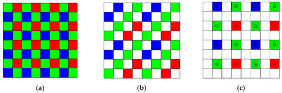
Figure 1.
Three CFA patterns. (a) CFA 1.0; (b) CFA 2.0; (c) CFA 3.0.
Researchers working on CFAs believe that CFA 2.0 is more suitable for taking images in low lighting environments. Recently, some researchers [11] have further explored the possibility of adding more white pixels to the CFA 2.0. The new pattern has 75% white pixels and the RGB pixels are randomly distributed among the remaining 25% pixels.
Motivated by the work in [11], we propose a simple CFA pattern in which the RGB pixels are evenly distributed, instead of using randomly distributed RGB pixels. In particular, as shown in Figure 1c, each 4 × 4 block has 75% or 12 white pixels, 12.5% or two green pixels, 6.25% or one red and blue pixels. We identify this CFA pattern as the CFA 3.0. There are three key advantages of using fixed CFA patterns. For the random pattern case, each camera will have a different pattern. In contrast, the first advantage is that the proposed fixed pattern allows a camera manufacturer to mass produce the cameras without changing the RGBW patterns for each camera. This can save manufacturing cost quite significantly. The second advantage is that the demosaicing software can be the same in all cameras if the pattern is fixed. Otherwise, each camera needs to have a unique demosaicing software tailored to a specific random pattern. This will seriously affect the cost. The third advantage is that some of the demosaicing algorithms for CFA 2.0 can be applied with little modifications. This can be easily seen if one puts the standard demosaicing block diagrams for CFA 2.0 and CFA 3.0 side by side. One can immediately notice that the reduced resolution color image and the panchromatic images can be similarly generated. As a result, the standard approach for CFA 2.0, all the pan-sharpening based algorithms for CFA 2.0, and the combination of pan-sharpening, and deep learning approaches for CFA 2.0, that we developed earlier in [12] can be applied to CFA 3.0.
In our recent paper on the demosaicing of CFA 2.0 (RGBW) [12], we have compared CFA 1.0 and CFA 2.0 using IMAX and Kodak images and observed that CFA 1.0 was better than CFA 2.0. One may argue that our comparison was not fair because IMAX and Kodak datasets were not collected in low lighting conditions and CFA 2.0 was designed for taking images in low lighting environments. Due to the dominance of white pixels in CFA 2.0, the SNR of the collected image is high and hence CFA 2.0 should have better demosaicing performance in dark environments.
Recently, we systematically and thoroughly compared CFA 1.0 and CFA 2.0 under dark conditions [13]. We observed that CFA 2.0 indeed performed better under dark conditions. We also noticed that denoising can further improve the demosaicing performance.
The aforementioned discussions immediately lead to several questions concerning the different CFAs. First, we enquired how demosaic CFA 3.0. Although there are universal debayering algorithms [8,9,10], those codes are not accessible to the public or may require customization. Here, we propose quite a few algorithms that can demosaic CFA 3.0, and this can be considered as our first contribution. Second, regardless of whether the answer to the first question is positive or negative, will more white pixels in the CFA pattern help the demosaicing performance for low lighting images? In other words, will CFA 3.0 have any advantages over CFA 1.0 and CFA 2.0? It will be a good contribution to the research community to answer the question: Which CFA out of the three is most suitable for low lighting environments? Third, the low lighting images contain Poisson noise and demosaicing does not have denoising capability. To improve the demosaicing performance, researchers usually carry out some denoising and contrast enhancement. It is important to know where one should perform denoising. Denoising can be performed either after or before demosaicing. Which choice can yield better overall image quality? Answering the above questions will assist designers understand the next generation of cameras that have adaptive denoising capability to handle diverse lighting environments.
In this paper, we will address the aforementioned questions. After some extensive research and experiments, we found that some algorithms for CFA 2.0 can be adapted to demosaic CFA 3.0. For instance, the standard approach for CFA 2.0 is still applicable to CFA 3.0. The pan-sharpening based algorithms for CFA 2.0 [12] and deep learning based algorithms for CFA 2.0 [14] are also applicable to CFA 3.0. We will describe those details in Section 2. In Section 3, we will first present experiments to demonstrate that CFA 3.0 can work well for low lighting images. Denoising using block matching in 3D (BM3D) [15] can further enhance the demosaicing performance. We also summarize a comparative study that compares the performance of CFA 1.0, CFA 2.0, and CFA 3.0 using normal and emulated low lighting images. We have several important findings. First, having more white pixels does not always improve the demosaicing performance. CFA 2.0 achieved the best performance. CFA 3.0 performs better than CFA 1.0 and is slightly inferior to CFA 2.0. Second, denoising can further enhance the demosaicing performance in all CFAs. Third, we observed that the final image quality relies heavily on the location of denoising. In particular, denoising after demosaicing is worse than denoising before demosaicing. Fourth, when the SNR is low, denoising has more influence on demosaicing. Some discussions on those findings are also included. In Section 4, some remarks and future research directions will conclude our paper.
2. Demosaicing Algorithms
We will first review some demosaicing algorithms for CFA 2.0. We will then answer the first question mentioned in Section 1: how one can demosaic the CFA 3.0 pattern shown in Figure 1c. It turns out that some of the existing algorithms for CFA 2.0 can be used for CFA 3.0 with some minor modifications.
2.1. Demosaicing Algorithms for CFA 2.0
The baseline approach is a simple demosaicing operation on the CFA, followed by an upsampling of the reduced resolution color image shown in Figure 2 of [13]. The standard approach consists of four steps as shown in Figure 2 of [13]. Step 1 interpolates the luminance image with half of the white pixels missing. Step 2 subtracts the reduced color image from the down-sampled interpolated luminance image. Step 3 upsamples the difference image in Step 2. Step 4 fuses the full resolution luminance with the upsampled difference image in Step 3. In our implementation, the demosaicing of the reduced resolution color image is done using local directional interpolation and nonlocal adaptive thresholding (LDI-NAT) [16] and the pan interpolation is also done using LDI-NAT [16].
In our recent paper [12], a pan-sharpening approach, as shown in Figure 2 of [13], was proposed to demosaicing CFA 2.0. The demosaicing of the reduced resolution color image is done using LDI-NAT [16]. The panchromatic (luminance) band with missing pixels is interpolated using LDI-NAT [16]. After those steps, pan-sharpening is performed to generate the full resolution color image. It should be noted that many pan-sharpening algorithms have been used in our experiments, including Principal Component Analysis (PCA) [17], Smoothing Filter-based Intensity Modulation (SFIM) [18], Modulation Transfer Function Generalized Laplacian Pyramid (GLP) [19], MTF-GLP with High Pass Modulation (HPM) [20], Gram Schmidt (GS) [21], GS Adaptive (GSA) [22], Guided Filter PCA (GFPCA) [23], PRACS [24] and hybrid color mapping (HCM) [25,26,27,28,29].
In a recent paper by us [14], the pan-sharpening approach has been improved by integrating with deep learning. As shown in Figure 4 of [13], a deep learning method was incorporated in two places. First, deep learning has been used to demosaic the reduced resolution CFA image. Second, deep learning has been used to improve the interpolation of the pan band. We adopted a deep learning algorithm known as Demonet [30]. Good performance improvement has been observed.
Moreover, the least-squares luma-chroma demultiplexing (LSLCD) [31] algorithm was used in our experiments for CFA 2.0.
In the past, we also developed two pixel-level fusion algorithms known as fusion of 3 (F3) algorithms and alpha trimmed mean filter (ATMF), which were used in our earlier studies [12,13,14,32]. Three best performing algorithms are fused in F3 and seven high performing algorithms are fused in ATMF. These fusion algorithms are applicable to any CFAs.
2.2. Demosaicing Algorithms for CFA 3.0
As opposed to the random color patterns in [11], the CFA 3.0 pattern in this paper has fixed patterns. One key advantage is that some of the approaches for CFA 2.0 can be easily applied with little modifications. For instance, the standard approach shown in Figure 2 of [13] for CFA 2.0 can be immediately applied to CFA 3.0, as shown in Figure 2. In each 4 × 4 block, the four R, G, B pixels in the CFA 3.0 raw image are extracted to form a reduced resolution CFA image. A standard demosaicing algorithm, any of those mentioned in Section 2.1 can be applied. In our implementation, we used LDI-NAT [16] for demosaicing the reduced resolution color image. The missing pan pixels are interpolated using LDI-NAT [16] to create a full resolution pan image. The subsequent steps will be the same as before.
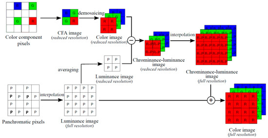
Figure 2.
Standard approach for CFA 3.0.
Similarly, the pan-sharpening approach for CFA 2.0 shown in Figure 3 of [13] can be applied to CFA 3.0 as shown in Figure 3. Here, the four R, G, B pixels are extracted first and then a demosaicing algorithm for CFA 1.0 is applied to the reduced resolution Bayer image. We used LDI-NAT [16] for reduced resolution color image. For the pan band, any interpolation algorithms can be applied. We used LDI-NAT. Afterwards, any pan-sharpening algorithms mentioned earlier can be used to fuse the pan and the demosaiced reduced resolution color image to generate a full resolution color image. In our experiments, we have used PCA [17], SFIM [18], GLP [19], HPM [20], GS [21], GSA [22], GFPCA [23], PRACS [24] and HCM [25] for pan-sharpening.
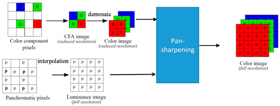
Figure 3.
A pan-sharpening approach for CFA 3.0.
The hybrid deep learning and pan-sharpening approach for CFA 2.0 shown in Figure 4 of [13] can be extended to CFA 3.0, as shown in Figure 4. For the reduced resolution demosaicing step, the Demonet algorithm is used. In the pan band generation step, we also propose to apply Demonet. The details are similar to our earlier paper on CFA 2.0 [12]. Hence, we skip the details. After those two steps, a pan-sharpening algorithm is then applied. In our experiments, Demonet is combined with different pan-sharpening algorithms in different scenarios. For normal lighting conditions, GSA is used for pan-sharpening and we call this hybrid approach the Demonet + GSA method. For low lighting conditions, it is more effective to use GFPCA for pan-sharpening and we term this as the Demonet + GFPCA method.
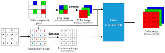
Figure 4.
A hybrid deep learning and pan-sharpening approach for CFA 3.0.
The two fusion algorithms (F3 and ATMF) can be directly applied to CFA 3.0.
2.3. Performance Metrics
Five performance metrics were used in our experiments to compare the different methods and CFAs. These metrics are well-known in the literature.
- Peak Signal-to-Noise Ratio (PSNR) [33]Separate PSNRs in dBs are computed for each band. A combined PSNR is the average of the PSNRs of the individual bands. Higher PSNR values imply higher image quality.
- Structural SIMilarity (SSIM)In [34], SSIM was defined to measure the closeness between two images. An SSIM value of 1 means that the two images are the same.
- Human Visual System (HVS) metricDetails of HVS metric in dB can be found in [35].
- HVSm (HVS with masking) [36]Similar to HVS, HVS incorporates the visual masking effects in computing the metrics.
- CIELABWe also used CIELAB [37] for assessing demosaicing and denoising performance in our experiments.
3. Experiments
In Section 2, we answer the first question about how one can demosaic CFA 3.0. Here, we will answer the two remaining questions mentioned in Section 1. One of the questions is whether or not the new CFA 3.0 can perform well for demosacing low lighting images. The other question is regarding whether CFA 3.0 has any advantages over the other two CFAs. Simply put, we will answer which one of the three CFAs is the best method for low light environments.
3.1. Data
A benchmark dataset (Kodak) was downloaded from a website (http://r0k.us/graphics/kodak/) and 12 images were selected. The images are shown in Figure 5 of [13]. We will use them as reference images for generating objective performance metrics. In addition, noisy images emulating images collected from dark conditions will be created using those clean images. It should be noted that the Kodak images were collected using films and then converted to digital images. We are absolutely certain that the images were not created using CFA 1.0. Many researchers in the demosaicing community have used Kodak data sets in their studies.
Emulating images in low lighting conditions is important because ground truth (clean) images can then be used for a performance assessment. In the literature, some researchers used Gaussian noise to emulate low lighting images. We think the proper way to emulate low lighting images is by using Poisson noise, which is simply because the noise introduced in low lighting images follows a Poisson distribution.
The differences between Gaussian and Poisson noises are explained as follows. Gaussian noise is additive, independent at each pixel, and independent of the pixel intensity. It is caused primarily by Johnson–Nyquist noise (thermal noise) [38]. Poisson noise is pixel intensity dependent and is caused by the statistical variation in the number of photons. Poisson noise is also known as photon shot noise [39]. As the number of photons at the detectors of cameras follows a Poisson distribution, and hence, the name of Poisson noise, when the number of photons increases significantly, the noise behavior then follows a Gaussian distribution due to the law of large numbers. However, the shot noise behavior of transitioning from Poisson distribution to Gaussian distribution does not mean that Poisson noise (photon noise) becomes Gaussian noise (thermal noise) when the number of photons increases significantly. This may be confusing for many people due to the terminology of Gaussian distribution. In short, the two noises come from different origins and have very different behaviors.
Poisson distribution has been widely used to characterize discrete events. For example, the arrival of customers to a bank follows a Poisson distribution; the number of phone calls to a cell phone tower also follows a Poisson distribution. For cameras, the probability density function (pdf) of photon noise in an image pixel follows a Poisson distribution, which can be mathematically described as,
where λ is the mean number of photons per pixel and P(k) is the probability when there are k photons. Based on the above pdf, one can interpret the actual number of photons arriving at a detector pixel fluctuates around the mean (λ), which can be used to characterize the lighting conditions. That is, a small λ implies the lighting is low and vice versa.
In statistics, when λ increases to a large number, the pdf in (1) will become a continuous pdf known as the Gaussian distribution, which is given by,
where x denotes the continuous noise variable and λ is the same for both mean and variance in Poisson noise. In [40], central limit theorem is used to connect (1) and (2) by assuming λ >> 1. The derivation of (2) from (1) can be found in [41]. Figure 5 [42] clearly shows that the Poisson distribution gradually becomes a Gaussian distribution when λ increases. It appears that when λ = 10, the Poisson pdf already looks like a Gaussian distribution.
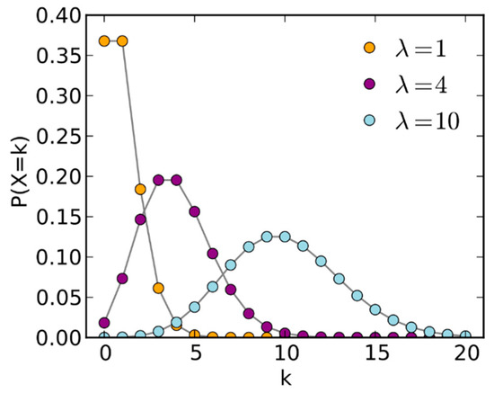
Figure 5.
Poisson distributions with varying .
However, it must be emphasized here that although (2) follows the normal or Gaussian distribution, the noise is still photon shot noise, not Gaussian noise due to thermal noise.
In contrast, Gaussian noise (thermal noise) follows the following distribution,
where z is the noise variable, μ is the mean, and σ is the standard deviation. As mentioned earlier, Gaussian noise is thermal noise and is independent of pixels and pixel intensity. To introduce Gaussian noise to a clean image, one can use a Matlab function: imnoise (I, “Gaussian”, μ, σ2) where I is a clean image and μ is set to zero.
Here, we describe a little more about the imaging model in low lighting conditions. As mentioned earlier, Poisson noise is related to the average number of photons per pixel, λ. To emulate the low lighting images, we vary λ. It should be noted that the SNR in dB of a Poisson image is given by [40]:
A number of images with different levels of Poisson noise or SNR can be seen in the table in Appendix A.
The process of how we introduced Poisson noise is adapted from code written by Erez Posner (https://github.com/erezposner/Shot-Noise-Generator) and it is summarized as follows.
Given a clean image and the goal of generating a Poisson noisy image with a target signal-to-noise (SNR) value in dB, we first compute the full-well (FW) capacity of the camera, which is related to the SNR through:
For a pixel I(i,j), we then compute the average photons per pixel (λ) for that pixel by,
where 255 is the number of intensity levels in an image. Using a Poisson noise function created by Donald Knuth [43], we can generate an actual photon number k through the Poisson distribution described by Equation (1). This k value changes randomly whenever a new call to the Poisson noise function is being made.
λ = I(i,j) × FW/255
Finally, the actual noisy pixel amplitude (In(i,j)) is given by:
In(i,j) = 255 × k/FW
A loop iterating over every (i,j) in the image will generate the noisy Poisson image with the target SNR value.
Although Gaussian and Poisson noises have completely different characteristics, it will be interesting to understand when the two noises will become indistinguishable. To achieve that and to save some space, we include noisy images between 20 dBs and 38 dBs. It should be noted that the Gaussian noise was generated using Matlab’s noise generation function (imnoise). The Poisson noise was generated following an open source code [44]. The SNRs are calculated by comparing the noisy images to the ground truth image. From Table A1 in Appendix A, we can see that when SNR values are less than 35 dBs, the two types of noisy images are visually different. Poisson images are slightly darker than Gaussian images. When SNR increases beyond 35 dBs, the two noisy images are almost indistinguishable.
From this study, we can conclude that 35-dB SNR is the threshold for differentiating Poisson noise (photon shot noise) from Gaussian noise (thermal). At 35 dBs, the average number of photons per pixel arriving at the detector is 3200 for Poisson noise and the standard deviation of the Gaussian noise is 0.0177. The image pixels are in double precision and normalized between 0 and 1.
To create a consistent level of noise close to our SNR levels of 10 dBs and 20 dBs, we followed a technique described in [44,45]. For each color band, we added Poisson noise separately. The noisy and low lighting images at 10 dBs and 20 dBs are shown in Figures 6 and 7 of [13], respectively.
In this paper, denoising is done via BM3D [15], which is a well-known method in the research community. The particular BM3D is specifically for Poisson noise. We performed denoising in a band by band manner. The BM3D package we used is titled ‘Denoising software for Poisson and Poisson-Gaussian data,” released on March 16th 2016. See the link (http://www.cs.tut.fi/~foi/invansc/). We used this code as packaged, which requires the input to be a single band image. This package would not require any input other than a single band noisy image. We considered using the standard BM3D package titled “BM3D Matlab” in this link (http://www.cs.tut.fi/~foi/GCF-BM3D/) released on February 16th 2020. This package would allow denoising 3-band RGB images. This package, however, assumes Gaussian noise and required a parameter based on the noise level.
3.2. CFA 3.0 Results
Here, we will first present demosaicing of CFA 3.0 for clean images, which are collected under normal lighting conditions. We will then present demosaicing of low lighting images at two SNRs with and without denoising.
3.2.1. Demosaicing Clean Images
There are 14 methods in our study. The baseline and standard methods are mentioned in Section 2.2. The other 12 methods include two fusion methods, one deep learning (Demonet + GSA), and nine pansharpening methods.
The three best methods used for F3 are Demonet + GSA, GSA, and GFPCA. The ATMF uses those three methods as well as Standard, PCA, GS, and PRACS.
From the PSNR and SSIM metrics in Table A2, the best performing algorithm is the Demonet + GSA method. The fusion methods of F3 and ATMF have better scores in Cielab, HVS and HVSm. Figure 6 shows the averaged metrics for all images.
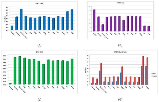
Figure 6.
Averaged performance metrics for all the clean images. (a) PNSR; (b) CIELAB; (c) SSIM; (d) HVS and HVSm.
In subjective comparisons shown in Figure 7, we can see the performance of the three selected methods (Demonet + GSA, ATMF and F3) varies a lot. Visually speaking, Demonet + GSA has the best visual performance. There are some minor color distortions in the fence area of the lighthouse image for F3 and ATMF.
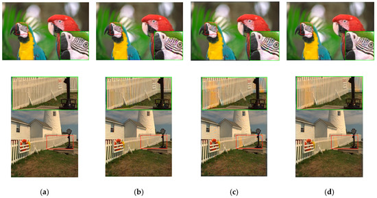
Figure 7.
Visual comparison of three high performing demosaicing algorithms. The top row is the bird image and the bottom row is the lighthouse image. (a) Ground Truth; (b) Demonet + GSA; (c) ATMF; (d) F3.
3.2.2. 10 dBs SNR
There are three cases in this sub-section. In the first case, we focus on the noisy images and there is no denoising. The second case includes denoising after demosaicing operation. The third case is about denoising before demosaicing operation.
● Case 1: No Denoising
There are 14 methods for demosaicing CFA 3.0. The F3 method is a fusion method that fused the results of Standard, Demonet+GFPCA, and GFPCA, which are the best performing individual methods for this case. The ATMF fusion method used the seven high performing methods, which are Standard, Demonet+GFPCA, GFPCA, Baseline, PCA, GS, and PRACS. Table A3 in Appendix A summarizes the PSNR, the CIELAB, SSIM, HVS, and HVSm metrics. The PSNR and CIELAB values vary a lot. All the SSIM, HVS, and HVSm values are not high.
The averaged PSNR, CIELAB, SSIM, HVS, and HVSm scores of all the 14 methods are shown in Figure 8. Big variations can be observed in the metrics.
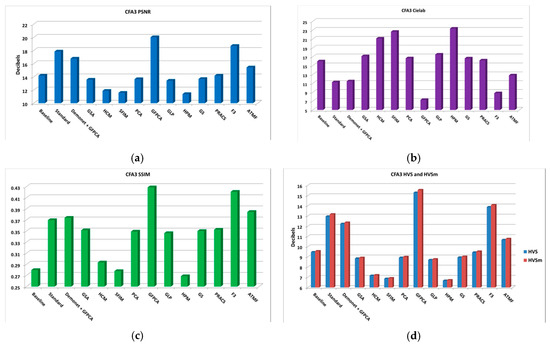
Figure 8.
Averaged performance metrics for all the low lighting images at 10 dBs SNR (Poisson noise). (a) PNSR; (b) CIELAB; (c) SSIM; (d) HVS and HVSm.
The demosaiced results of Images 1 and 8 are shown in Figure 9. There are color distortion, noise, and contrast issues in the demosaiced images.
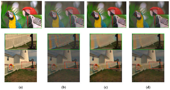
Figure 9.
Visual comparison of three high performing demosaicing algorithms at 10 dBs SNR (Poisson noise). The top row is the bird image and the bottom row is the lighthouse image. (a) Ground Truth; (b) Standard; (c) GFPCA; (d) F3.
It can be observed that, if there is no denoising, all the algorithms have big fluctuations and the demosaiced results are not satisfactory.
● Case 2: Denoising after Demosaicing
In this case, we applied demosaicing first, followed by denoising. The denoising algorithm is BM3D. The denoising was done one band at a time. The F3 method fused the results from Demonet + GFPCA, GFPCA, and GSA. ATMF fused results from Demonet + GFPCA, GFPCA, GSA, PCA, GLP, GS, and PRACS. From Table A4 in Appendix A, the averaged PSNR score of Demonet + GFPCA and GFPCA have much higher scores than the rest. The other methods also yielded around 4 dBs higher scores than those numbers in Table A3.
Figure 10 illustrates the averaged performance metrics, which look much better than those in Figure 8.
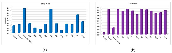
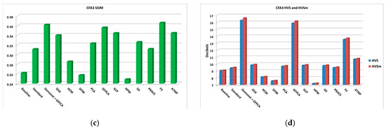
Figure 10.
Averaged performance metrics for all the low light images at 10 dBs SNR (Poisson noise). (a) PNSR; (b) CIELAB; (c) SSIM; (d) HVS and HVSm.
The denoised and demosaiced images of three methods are shown in Figure 11. We observe that the artifacts in Figure 9 have been reduced significantly. Visually speaking, the distortion in the images of Demonet + GFPCA is quite small for the fence area of Image 8.
Figure 11.
Visual comparison of three high performing demosaicing algorithms at 10 dBs SNR (Poisson noise). The top row is the bird image and the bottom row is the lighthouse image. (a) Ground Truth; (b) Demonet + GFPCA; (c) ATMF; (d) F3.
● Case 3: Denoising before Demosaicing
In this case, we first performed denoising and then demosaicing by pansharpening. The denoising is applied to two places. One is to the luminance image, which is the image after interpolation. The other place is to the reduced resolution color image. Denoising using Akiyama et al. approach [46] is a good alternative and will be a good future direction. The F3 method fused the results from the Standard, Demonet + GFPCA, GSA. ATMF fused the results from Standard, Demonet + GFPCA, GSA, HCM, GFPCA, GLP, and PRACS. From Table A5, we can see that the Demonet + GFPCA algorithm yielded the best averaged PSNR score, which is close to 26 dBs. This is almost 6 dBs better than those numbers in Table A4 and 16 dBs more than those in Table A3. The other metrics in Table A5 are all significantly improved over Table A4. As we will explain later, denoising after demosaicing performs worse than that of before demosaicing.
Figure 12 shows the averaged performance metrics. The metrics are significantly better than those in Figure 8 and Figure 10.
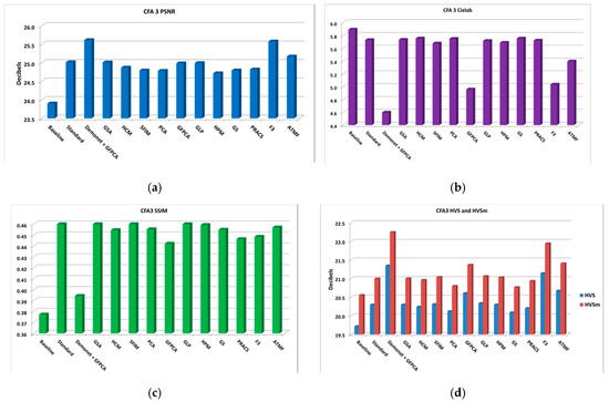
Figure 12.
Averaged performance metrics for all the low light images at 10 dBs SNR (Poisson noise). (a) PNSR; (b) CIELAB; (c) SSIM; (d) HVS and HVSm.
Figure 13 shows the demosaiced images of three methods. We can observe that the demosaiced images have better contrast than those in Figure 11. The Demonet + GFPCA method has less color distortion.
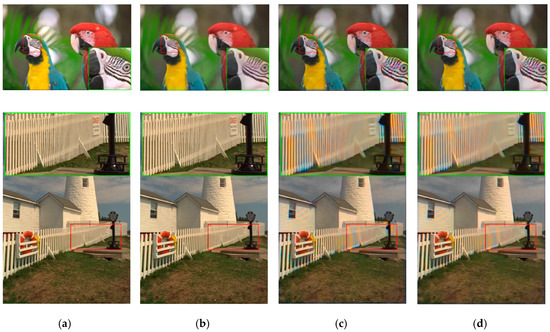
Figure 13.
Visual comparison of three high performing demosaicing algorithms at 10 dBs SNR (Poisson noise). The top row is the bird image and the bottom row is the lighthouse image. (a) Ground Truth; (b) Demonet + GFPCA; (c) ATMF; (d) F3.
3.2.3. 20 dBs SNR
We have three cases here.
● Case 1: No Denoising (20 dBs SNR)
There are 14 methods. The F3 method fused the three best performing methods: Demonet+GFPCA, GFPCA, and PRACS. ATMF fused the seven best performing methods: Demonet+GFPCA, GFPCA, PRACS, Baseline, GSA, PCA, and GLP. From Table A6 in Appendix A, we can see that the averaged PSNR score of PRACS is the best, which is 21.8 dBs.
The average performance metrics are shown in Figure 14. The results are reasonable because there is no denoising capability in demosaicing methods. Figure 15 shows the demosaiced images of three methods: GFPCA, ATMF, and F3. One can easily see some artifacts (color distortion).
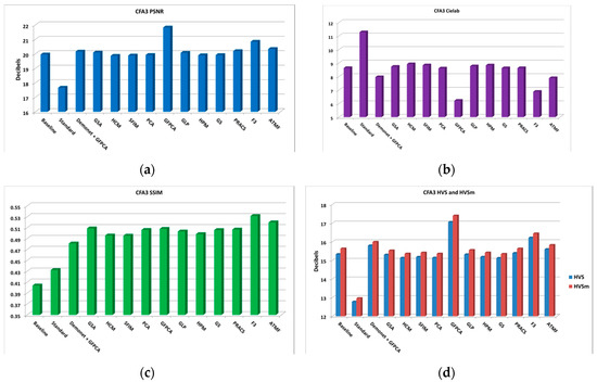
Figure 14.
Averaged performance metrics for all the low light images at 20 dBs SNR (Poisson noise). (a) PNSR; (b) CIELAB; (c) SSIM; (d) HVS and HVSm.
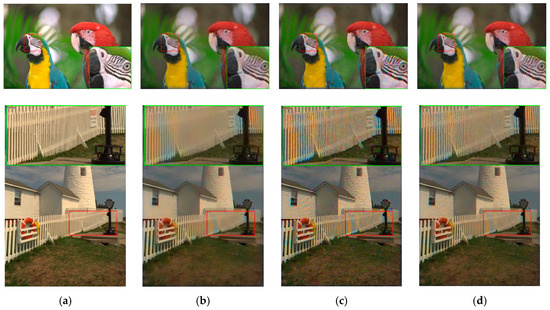
Figure 15.
Visual comparison of three high performing demosaicing algorithms at 20 dBs SNR (Poisson noise). The top row is the bird image and the bottom row is the lighthouse image. (a) Ground Truth; (b) GFPCA; (c) ATMF; (d) F3.
● Case 2: Denoising after Demosaicing (20 dBs SNR)
The F3 method performed pixel level fusion using the results of Demonet + GFPCA, GFPCA, and GLP. ATMF fused the results of Demonet + GFPCA, GFPCA, GLP, Standard, GSA, PCA, and GS. From Table A7, we can observe that the Demonet + GFPCA achieved the highest averaged PSNR score of 21.292 dBs. This is better than most of PSNR numbers in Table A6, but only slightly better than the Demonet + GFPCA method (20.573 dBs) in Table A4 (10 dBs SNR case). This clearly shows that denoising has more dramatic impact for low SNR case than with high SNR case. The other metrics in Table A7 are all improved over those numbers in Table A6.
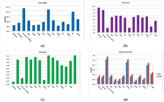
Figure 16.
Averaged performance metrics for all the low light images at 20 dBs SNR (Poisson noise). (a) PNSR; (b) CIELAB; (c) SSIM; (d) HVS and HVSm.
The demosaiced images of three methods are shown in Figure 17. We can see that the artifacts in Figure 17 have been reduced as compared to Figure 15. The color distortions are still noticeable.
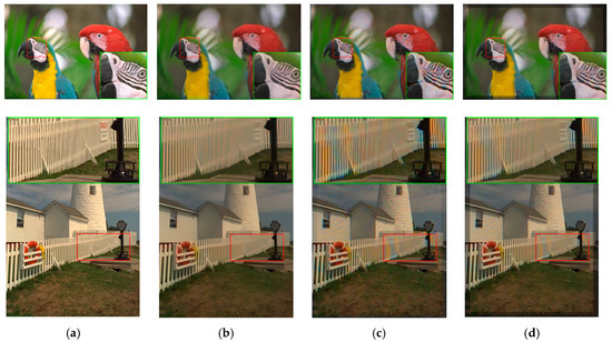
Figure 17.
Visual comparison of three high performing demosaicing algorithms at 20 dBs SNR (Poisson noise). The top row is the bird image and the bottom row is the lighthouse image. (a) Ground Truth; (b) Demonet + GFPCA; (c) ATMF; (d) F3.
● Case 3: Denoising before Demosaicing (20 dBs SNR)
The F3 method fused the results of three best performing methods: Standard, GSA, and GFPCA. ATMF fused the 7 best performing methods: Standard, GSA, GFPCA, HCA, SFIM, GS, and HPM. From Table A8, we can see that F3 yielded 27.07 dBs of PSNR. This is 7 dBs better than the best method in Table A6 and 6 dBs better than the best method in Table A7. The other metrics in Table A8 are all improved over Table A7 quite significantly. This means that the location of denoising is quite critical for improving the overall demosaicing performance.
Figure 18 shows the average performance metrics. The numbers are better than those in Figure 14 and Figure 16.
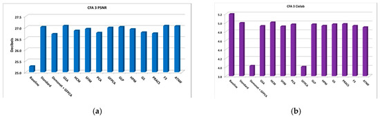
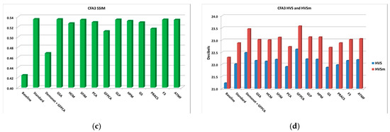
Figure 18.
Averaged performance metrics for all the low light images at 20 dBs SNR (Poisson noise). (a) PNSR; (b) CIELAB; (c) SSIM; (d) HVS and HVSm.
Figure 19 displays the demosaiced images of three selected methods. It is hard to say whether or not the demosaiced images in Figure 19 is better than that of Figure 17 because there are some color distortions.
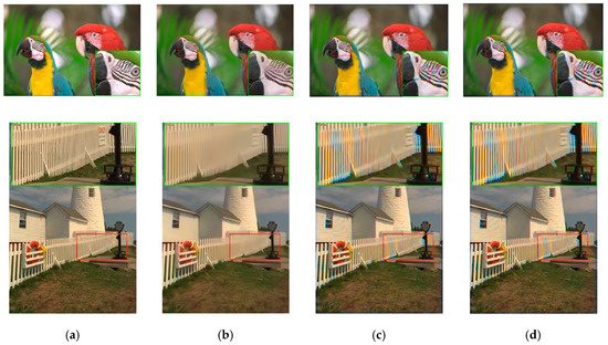
Figure 19.
Visual comparison of three high performing demosaicing algorithms at 20 dBs SNR (Poisson noise). The top row is the bird image and the bottom row is the lighthouse image. (a) Ground Truth; (b) Demonet + GFPCA; (c)ATMF; (d) F3.
3.3. Comparison of CFAs 1.0, 2.0, and 3.0
As mentioned in Section 1, it will be important to compare the three CFAs and answer the question; which is the best for low lighting images? Given that different algorithms were used in each CFA, selecting the best performing method for each CFA and comparing them against one another will be a good strategy.
We evaluated the following algorithms for CFA 1.0 d in our experiments. Three of them are deep learning based algorithms (Demonet, SEM, and DRL).
- Linear Directional Interpolation and Nonlocal Adaptive Thresholding (LDI-NAT) [16].
- Demosaicnet (Demonet) [30].
- Fusion using 3 best (F3) [32].
- Bilinear [47].
- Malvar–He–Cutler (MHC) [47].
- Directional Linear Minimum Mean Square-Error Estimation (DLMMSE) [48].
- Lu and Tan Interpolation (LT) [49].
- Adaptive Frequency Domain (AFD) [50].
- Alternate Projection (AP). [51].
- Primary-Consistent Soft-Decision (PCSD) [52].
- Alpha Trimmed Mean Filtering (ATMF) [32,53].
- Sequential Energy Minimization (SEM) [54].
- Deep Residual Network (DRL) [55].
- Exploitation of Color Correlation (ECC) [56].
- Minimized-Laplacian Residual Interpolation (MLRI) [57].
- Adaptive Residual Interpolation (ARI) [58].
- Directional Difference Regression (DDR) [59].
3.3.1. Noiseless Case (Normal Lighting Conditions)
Here, we compare the performance of CFAs in the noiseless case. The 12 clean Kodak images were used in our study. To save space, we do not provide the image by image performance metrics. Instead, we only summarize the averaged metrics of the different CFAs in Table 1 and Figure 20. In each cell of Table 1, we provide the metric values as well as the name of the best performance method for that metric. One can see that CFA 1.0 is the best in every performance metric, followed by CFA 2.0. CFA 3.0 has the worst performance. We had the same observation for CFA 1.0 and CFA 2.0 in our earlier studies [12].

Table 1.
Comparison of CFAs for different demosaicing method in the noiseless case (normal lighting conditions). Bold numbers indicate the best performing methods in each row.
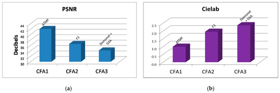
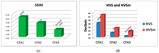
Figure 20.
Best against the best comparison between CFAs 1.0, 2.0, and 3.0 in the noiseless case. (a) PSNR metrics; (b) Cielab metrics; (c) SSIM metrics; (d) HVS and HVSm metrics.
3.3.2. 10 dBs SNR
Table 2 and Figure 21 summarize the averaged performance metrics for 10 dBs SNR case in our earlier studies in Section 3.2 for CFA 3.0 and our earlier paper [13] for CFAs 1.0 and 2.0. In Table 2, we include the name of the best performing algorithm. We have the following observations:
Table 2.
Comparison of CFA patterns for the various demosaicing cases at 10 dBs SNR. Bold numbers indicate the best performing methods in each row.
Figure 21.
Best against the best comparison between CFAs 1.0, 2.0, and 3.0 with and without denoising at 10 dBs SNR. (a) PSNR metrics; (b) Cielab metrics; (c) SSIM metrics; (d) HVS metrics; (e) HVSm metrics.
- Without denoising, CFAs 1.0, 2.0, and 3.0 have big differences. CFA 2.0 is more than 4 dBs higher than CFA 1.0 and CFA 3.0 is 1.2 dBs lower than CFA 2.0.
- Denoising improves the demosaicing performance independent of the denoising location. For CFA 1.0, the improvement over no denoising is 4 dBs; for CFA 2.0, the improvement is more than 2.7 dBs to 5 dBs; for CFA 3.0, we see 0.57 dBs to 5.6 dBs of improvement in PSNR. We also see dramatic improvements in other metrics,
- Denoising after demosaicing is worse than that of denoising before demosaicing. For CFA 1.0, the improvement is 1.1 dBs with denoising before demosaicing; for CFA 2.0, the improvement is 2.1 dBs with denoising before demosaicing; for CFA 3.0, the improvement is over 5 dBs in PSNR with denoising before demosaicing.
- One important finding is that CFAs 2.0 and 3.0 definitely have advantages over CFA 1.0.
- CFA 2.0 is better than CFA 3.0.
3.3.3. 20 dBs SNR
In Table 3 and Figure 22, we summarize the best results for different CFAs under different denoising/demosaicing scenarios presented in earlier sections. Some numbers for CFAs 1.0 and 2.0 in Table 3 came from our earlier paper [13]. The following observations can be drawn:
Table 3.
Comparison of CFA patterns for the various demosaicing cases at 20 dBs SNR. Bold numbers indicate the best performing methods in each row.
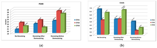
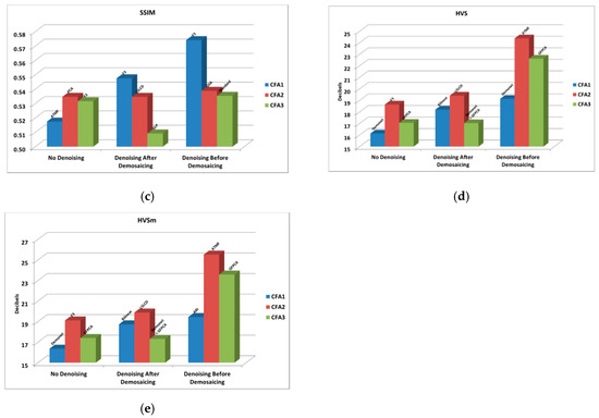
Figure 22.
Best against the best comparison between CFAs 1.0, 2.0, and 3.0 with and without denoising at 20 dBs SNR. (a) PSNR metrics; (b) Cielab metrics; (c) SSIM metrics; (d) HVS metrics; (e) HVSm metrics.
- Without denoising, CFA 2.0 is the best, followed by CFA 3.0 and CFA 1.0.
- Denoising improves the demosaicing performance in all scenarios. For CFA 1.0, the improvement is over 2 to 4 dBs; for CFA 2.0, the improvement is more than 1 to close to 5 dBs; for CFA 3.0, the improvement is 6 dBs in terms of PSNR. Other metrics have been improved with denoising.
- Denoising after demosaicing is worse than that of denoising before demosaicing. For CFA 1.0, the improvement is 1.2 dBs with denoising before demosaicing; for CFA 2.0, the improvement is close to 4 dBs with denoising before demosaicing; for CFA 3.0, the improvement is close to 6 dBs in PSNR with denoising before demosaicing.
- We observe that CFAs 2.0 and 3.0 definitely have advantages over CFA 1.0.
- CFA 2.0 is better than CFA 3.0.
3.4. Discussions
Here, some qualitative analyses/explanations for some of those important findings in Section 3.3.2 and Section 3.3.3 are provided:
● The reason denoising before demosaicing is better that after demosaicing
We explained this phenomenon in our earlier paper [13]. The reason is simply because noise is easier to suppress early than later. Once noise has propagated down the processing pipeline, it is harder to suppress it due to some nonlinear processing modules. For instance, the rectified linear units (ReLu) are nonlinear in some deep learning methods. We have seen similar noise behavior in our active noise suppression project for NASA. In that project [60,61], we noticed that noise near the source was suppressed more effectively than noise far away from the source.
● The reasons why CFA 2.0 and CFA 3.0 are better than CFA 1.0 in low lighting conditions
To the best of our knowledge, we are not aware of any theory explaining why CFA 2.0 and CFA 3.0 have better performance than CFA 1.0. Intuitively, we agree with the inventors of CFA 2.0 that having more white pixels improves the sensitivity of the imager/detector. Here, we offer another explanation.
We use the bird image at 10 dBs condition (Image 1 in Figure 6 of [13]) for explanations. Denoising was not used in the demosaicing process. Figure 23 contains three histograms and the means of the residual images (residual = reference − demosaiced) for CFAs 1.0, 2.0, and 3.0 are also computed. We can see that the histograms of CFA 2.0 and CFA 3.0 are centered near zero whereas the histogram of CFA 1.0 is biased towards to right, meaning that CFA 2.0 and CFA 3.0 are closer to the ground truth, because of their better light sensitivity, than that of CFA 1.0.
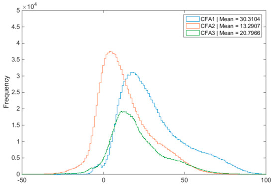
Figure 23.
No denoising cases at 10 dBs. Error distributions of the three CFAs.
● Why CFA 3.0 is NOT better than CFA 2.0 in low lighting conditions
We observe that CFA 3.0 is better than CFA 1.0, but is slightly inferior to CFA 2.0 in dark conditions, which means that having more white pixels can only improve the demosaicing performance to certain extent. Too many white pixels means fewer color pixels and this may degrade the demosaicing performance by having more color distortion. CFA 2.0 is the best compromise between sensitivity and color distortion.
4. Conclusions
In this paper, we first introduce a RGBW pattern with 75% of the pixels white, 12.5% of the pixels green, and 6.25% of the pixels red and blue. This is known as the CFA 3.0. Unlike a conventional RGBW pattern with 75% white and the rest pixels are randomly red, green and blue, our pattern is fixed. One key advantage of our pattern is that some of the algorithms for demosaicing CFA 2.0 can be easily adapted to CFA 3.0. Other advantages are also mentioned in Section 1. We then performed extensive experiments to evaluate the CFA 3.0 using clean and emulated low lighting images. After that, we compared the CFAs for various clean and noisy images. Using five objective performance metrics and subjective evaluations, it was observed that, the demosacing performance in CFA 2.0 and CFA 3.0 is indeed better than CFA 1.0. However, more white pixels do not guarantee better performance because CFA 3.0 is slightly worse than CFA 2.0. This is because the color information is less in CFA 3.0, compared to CFA 2.0, causing the loss of color information in the CFA 3.0 case. Denoising further improves the demosaicing performance. In our research, we have experimented with two denoising scenarios: before and after demosaicing. We have seen dramatic performance gain of more than 3 dBs improvement in PSNR for the 10 dBs case when denoising was applied. One important observation is that denoising after demosaicing is worse than denoising before demosaicing. Another observation is that CFA 2.0 with denoising is the best performing algorithm for low lighting conditions.
One potential future direction for research is to investigate different denoising algorithms, such as color BM3D and deep learning based denoising algorithms [62]. Another direction is to investigate joint denoising and demosaicing for CFAs 2.0 and 3.0 directly. Notably, joint denoising and demosaicing has been mostly done for CFA 1.0. The extension of joint denoising and demosaicing to CFAs 2.0 and 3.0 may be non-trivial and needs some further research.
Author Contributions
C.K. conceived the overall concept and wrote the paper. J.L. implemented the algorithm, prepared all the figures and tables. B.A. helped with the Poisson noise generation. All authors have read and agreed to the published version of the manuscript.
Funding
This research was supported by NASA JPL under contract # 80NSSC17C0035. The views, opinions and/or findings expressed are those of the author(s) and should not be interpreted as representing the official views or policies of NASA or the U.S. Government.
Acknowledgments
We would like to thank the anonymous reviewers for their constructive comments and suggestions, which significantly improved the quality of our paper.
Conflicts of Interest
The authors declare no conflict of interest.
Appendix A
Table A1.
Comparison of Gaussian and Poisson noisy images.
Table A1.
Comparison of Gaussian and Poisson noisy images.
| SNR | Images with Different Levels of Gaussian Noise (Thermal Noise) | Images with Different Levels of Poisson Noise (Photon Shot Noise) |
|---|---|---|
| 20 dB |  |  |
| σ = 0.1 | λ: average number of photons per pixel = 100 | |
| 23 dB |  |  |
| σ = 0.0707 | λ: average number of photons per pixel = 200 | |
| 26 dB |  |  |
| σ = 0.05 | λ: average number of photons per pixel = 400 | |
| 29 dB |  |  |
| σ = 0.0354 | λ: average number of photons per pixel = 800 | |
| 32 dB |  |  |
| σ = 0.025 | λ: average number of photons per pixel = 1600 | |
| 35 dB |  |  |
| σ = 0.0177 | λ: average number of photons per pixel = 3200 | |
| 38 dB |  |  |
| σ = 0.0125 | λ: average number of photons per pixel = 6400 |
Table A2.
Performance metrics of 14 algorithms for clean images. Bold numbers indicate the best performing method in each row. Red numbers indicate those methods used in F3 and those red and green numbers indicate those methods used in ATMF. Bold numbers indicate the best performing methods in each row.
| Image | Metrics | Baseline | Standard | Demonet + GSA | GSA | HCM | SFIM | PCA | GFPCA | GLP | HPM | GS | PRACS | F3 | ATMF | Best Score |
|---|---|---|---|---|---|---|---|---|---|---|---|---|---|---|---|---|
| Img1 | PSNR | 31.936 | 33.894 | 35.192 | 34.126 | 33.526 | 33.123 | 33.828 | 33.158 | 33.810 | 33.066 | 34.130 | 33.466 | 36.171 | 37.716 | 37.716 |
| Cielab | 2.659 | 2.374 | 2.250 | 2.393 | 2.481 | 2.699 | 2.445 | 2.773 | 2.429 | 2.724 | 2.351 | 2.453 | 1.853 | 1.560 | 1.560 | |
| SSIM | 0.739 | 0.859 | 0.832 | 0.854 | 0.831 | 0.838 | 0.845 | 0.806 | 0.853 | 0.834 | 0.858 | 0.820 | 0.839 | 0.857 | 0.859 | |
| HVS | 28.233 | 27.610 | 29.428 | 28.438 | 28.309 | 28.453 | 28.481 | 27.947 | 28.353 | 28.468 | 28.403 | 28.407 | 32.176 | 33.731 | 33.731 | |
| HVSm | 29.767 | 29.031 | 31.056 | 29.881 | 29.830 | 29.975 | 29.934 | 28.834 | 29.822 | 29.983 | 29.836 | 29.868 | 34.065 | 36.274 | 36.274 | |
| Img2 | PSNR | 26.771 | 30.585 | 34.464 | 30.581 | 30.211 | 29.918 | 30.406 | 30.136 | 30.089 | 29.896 | 30.521 | 30.230 | 30.737 | 32.027 | 34.464 |
| Cielab | 4.860 | 3.766 | 2.416 | 3.803 | 3.874 | 3.901 | 3.891 | 3.219 | 3.906 | 3.904 | 3.830 | 3.903 | 2.826 | 2.738 | 2.416 | |
| SSIM | 0.685 | 0.868 | 0.885 | 0.867 | 0.856 | 0.856 | 0.845 | 0.823 | 0.857 | 0.853 | 0.850 | 0.852 | 0.825 | 0.858 | 0.885 | |
| HVS | 23.976 | 24.331 | 30.067 | 24.486 | 24.304 | 24.264 | 24.726 | 27.637 | 24.398 | 24.228 | 24.403 | 24.445 | 28.565 | 28.822 | 30.067 | |
| HVSm | 25.515 | 25.629 | 32.745 | 25.803 | 25.665 | 25.666 | 26.076 | 29.840 | 25.721 | 25.613 | 25.703 | 25.762 | 31.724 | 31.215 | 32.745 | |
| Img3 | PSNR | 30.815 | 33.017 | 34.369 | 32.997 | 32.156 | 32.420 | 32.995 | 34.055 | 32.698 | 32.395 | 33.037 | 32.648 | 35.838 | 36.886 | 36.886 |
| Cielab | 3.758 | 3.378 | 2.836 | 3.313 | 3.535 | 3.432 | 3.324 | 2.949 | 3.345 | 3.459 | 3.303 | 3.398 | 2.196 | 1.907 | 1.907 | |
| SSIM | 0.786 | 0.888 | 0.880 | 0.884 | 0.870 | 0.879 | 0.877 | 0.873 | 0.878 | 0.873 | 0.877 | 0.870 | 0.883 | 0.894 | 0.894 | |
| HVS | 27.087 | 27.099 | 28.646 | 27.266 | 27.081 | 27.211 | 27.403 | 29.897 | 27.192 | 27.218 | 27.366 | 27.221 | 32.691 | 33.472 | 33.472 | |
| HVSm | 28.861 | 28.734 | 30.760 | 28.928 | 28.894 | 28.976 | 29.065 | 31.435 | 28.870 | 28.973 | 29.023 | 28.900 | 35.473 | 36.595 | 36.595 | |
| Img4 | PSNR | 22.762 | 26.980 | 30.511 | 27.496 | 27.090 | 26.808 | 26.884 | 26.873 | 26.762 | 26.771 | 26.884 | 26.933 | 29.365 | 29.546 | 30.511 |
| Cielab | 7.484 | 5.434 | 3.775 | 5.327 | 5.178 | 5.314 | 5.662 | 4.841 | 5.664 | 5.364 | 5.644 | 5.371 | 3.585 | 3.597 | 3.585 | |
| SSIM | 0.752 | 0.925 | 0.946 | 0.925 | 0.919 | 0.915 | 0.901 | 0.891 | 0.913 | 0.911 | 0.903 | 0.913 | 0.914 | 0.925 | 0.946 | |
| HVS | 20.315 | 20.370 | 25.427 | 21.077 | 21.064 | 21.160 | 20.986 | 24.117 | 21.095 | 21.203 | 20.867 | 20.918 | 26.657 | 25.799 | 26.657 | |
| HVSm | 21.997 | 21.682 | 27.751 | 22.476 | 22.526 | 22.656 | 22.377 | 26.303 | 22.547 | 22.706 | 22.240 | 22.337 | 29.826 | 28.261 | 29.826 | |
| Img5 | PSNR | 30.816 | 34.107 | 36.762 | 33.952 | 33.686 | 33.558 | 33.825 | 34.541 | 33.694 | 33.469 | 34.132 | 33.766 | 36.599 | 37.045 | 37.045 |
| Cielab | 2.568 | 2.100 | 1.593 | 2.172 | 2.054 | 2.107 | 2.180 | 1.914 | 2.132 | 2.123 | 2.070 | 2.136 | 1.488 | 1.459 | 1.459 | |
| SSIM | 0.668 | 0.868 | 0.858 | 0.852 | 0.859 | 0.859 | 0.845 | 0.798 | 0.855 | 0.852 | 0.859 | 0.838 | 0.816 | 0.827 | 0.868 | |
| HVS | 27.733 | 27.824 | 31.730 | 28.155 | 28.083 | 28.083 | 28.344 | 30.514 | 28.154 | 28.083 | 28.132 | 28.146 | 33.628 | 33.670 | 33.670 | |
| HVSm | 29.444 | 29.335 | 34.093 | 29.707 | 29.676 | 29.772 | 29.912 | 32.085 | 29.750 | 29.775 | 29.662 | 29.688 | 36.534 | 36.333 | 36.534 | |
| Img6 | PSNR | 27.706 | 30.874 | 33.168 | 31.031 | 30.391 | 30.382 | 30.980 | 31.381 | 30.647 | 30.278 | 30.926 | 30.601 | 32.511 | 33.125 | 33.168 |
| Cielab | 5.555 | 4.605 | 3.393 | 4.721 | 4.528 | 4.464 | 4.657 | 3.797 | 4.619 | 4.544 | 4.698 | 4.575 | 3.004 | 3.049 | 3.004 | |
| SSIM | 0.711 | 0.896 | 0.909 | 0.879 | 0.877 | 0.881 | 0.864 | 0.848 | 0.882 | 0.873 | 0.860 | 0.869 | 0.870 | 0.890 | 0.909 | |
| HVS | 24.678 | 24.823 | 27.010 | 25.114 | 24.877 | 25.031 | 25.034 | 27.599 | 25.159 | 25.047 | 25.097 | 24.967 | 28.985 | 29.193 | 29.193 | |
| HVSm | 26.353 | 26.293 | 28.953 | 26.606 | 26.470 | 26.603 | 26.520 | 29.306 | 26.665 | 26.611 | 26.591 | 26.495 | 31.643 | 31.803 | 31.803 | |
| Img7 | PSNR | 30.446 | 34.517 | 38.658 | 34.469 | 34.081 | 33.701 | 34.351 | 33.767 | 33.917 | 33.680 | 34.391 | 34.183 | 34.389 | 35.691 | 38.658 |
| Cielab | 3.639 | 2.751 | 1.687 | 2.773 | 2.809 | 2.855 | 2.799 | 2.501 | 2.854 | 2.857 | 2.785 | 2.841 | 2.141 | 2.078 | 1.687 | |
| SSIM | 0.731 | 0.904 | 0.920 | 0.903 | 0.896 | 0.894 | 0.897 | 0.853 | 0.894 | 0.891 | 0.897 | 0.892 | 0.861 | 0.894 | 0.920 | |
| HVS | 27.968 | 28.395 | 34.885 | 28.409 | 28.323 | 28.199 | 28.497 | 32.017 | 28.321 | 28.159 | 28.411 | 28.415 | 32.584 | 32.357 | 34.885 | |
| HVSm | 29.538 | 29.687 | 37.761 | 29.696 | 29.661 | 29.579 | 29.800 | 34.461 | 29.628 | 29.517 | 29.706 | 29.727 | 36.020 | 34.752 | 37.761 | |
| Img8 | PSNR | 26.939 | 30.748 | 33.682 | 31.078 | 30.419 | 30.253 | 30.568 | 30.319 | 30.390 | 30.123 | 30.670 | 30.439 | 33.479 | 33.700 | 33.700 |
| Cielab | 4.697 | 3.707 | 2.707 | 3.566 | 3.769 | 3.704 | 3.758 | 3.200 | 3.746 | 3.734 | 3.707 | 3.812 | 2.407 | 2.441 | 2.407 | |
| SSIM | 0.733 | 0.900 | 0.910 | 0.899 | 0.885 | 0.890 | 0.883 | 0.860 | 0.891 | 0.886 | 0.888 | 0.877 | 0.880 | 0.890 | 0.910 | |
| HVS | 24.460 | 24.087 | 28.285 | 25.013 | 24.854 | 24.969 | 25.039 | 28.845 | 25.004 | 24.996 | 24.866 | 24.883 | 31.045 | 29.955 | 31.045 | |
| HVSm | 26.141 | 25.461 | 30.690 | 26.453 | 26.378 | 26.496 | 26.473 | 30.948 | 26.476 | 26.519 | 26.277 | 26.335 | 34.113 | 32.146 | 34.113 | |
| Img9 | PSNR | 29.775 | 32.268 | 34.974 | 32.682 | 32.117 | 31.742 | 32.676 | 33.783 | 32.316 | 31.669 | 32.668 | 32.318 | 35.220 | 35.620 | 35.620 |
| Cielab | 3.062 | 2.705 | 2.017 | 2.592 | 2.601 | 2.911 | 2.561 | 2.202 | 2.669 | 2.974 | 2.566 | 2.595 | 1.707 | 1.683 | 1.683 | |
| SSIM | 0.508 | 0.634 | 0.643 | 0.637 | 0.623 | 0.623 | 0.582 | 0.615 | 0.577 | 0.564 | 0.582 | 0.616 | 0.624 | 0.631 | 0.643 | |
| HVS | 26.329 | 26.028 | 29.823 | 26.753 | 26.632 | 26.808 | 26.748 | 30.150 | 26.823 | 26.820 | 26.779 | 26.621 | 32.389 | 32.588 | 32.588 | |
| HVSm | 27.955 | 27.482 | 31.906 | 28.234 | 28.181 | 28.362 | 28.228 | 31.987 | 28.331 | 28.365 | 28.264 | 28.115 | 35.387 | 35.453 | 35.453 | |
| Img10 | PSNR | 27.054 | 30.354 | 33.931 | 30.547 | 29.970 | 29.885 | 30.350 | 31.177 | 30.014 | 29.822 | 30.309 | 30.118 | 31.819 | 32.689 | 33.931 |
| Cielab | 4.808 | 3.975 | 2.552 | 3.930 | 3.927 | 3.915 | 3.991 | 3.223 | 4.075 | 3.940 | 3.959 | 3.936 | 2.625 | 2.598 | 2.552 | |
| SSIM | 0.687 | 0.867 | 0.868 | 0.867 | 0.856 | 0.857 | 0.832 | 0.802 | 0.858 | 0.853 | 0.855 | 0.848 | 0.825 | 0.848 | 0.868 | |
| HVS | 24.184 | 24.135 | 28.936 | 24.517 | 24.440 | 24.459 | 24.450 | 28.393 | 24.508 | 24.441 | 24.515 | 24.458 | 29.661 | 29.396 | 29.661 | |
| HVSm | 25.796 | 25.521 | 31.336 | 25.928 | 25.963 | 25.969 | 25.867 | 30.357 | 25.931 | 25.936 | 25.935 | 25.910 | 33.182 | 32.163 | 33.182 | |
| Img11 | PSNR | 29.027 | 32.011 | 33.458 | 32.234 | 31.703 | 31.707 | 32.121 | 31.682 | 31.835 | 31.655 | 32.143 | 31.687 | 33.209 | 33.702 | 33.702 |
| Cielab | 4.282 | 3.556 | 3.004 | 3.529 | 3.654 | 3.606 | 3.545 | 3.412 | 3.628 | 3.627 | 3.543 | 3.605 | 2.753 | 2.686 | 2.686 | |
| SSIM | 0.722 | 0.882 | 0.894 | 0.883 | 0.866 | 0.875 | 0.875 | 0.840 | 0.875 | 0.871 | 0.876 | 0.862 | 0.861 | 0.877 | 0.894 | |
| HVS | 26.763 | 26.320 | 28.596 | 27.143 | 27.134 | 27.175 | 27.080 | 28.744 | 27.177 | 27.215 | 27.085 | 27.089 | 30.413 | 30.445 | 30.445 | |
| HVSm | 28.417 | 27.778 | 30.488 | 28.626 | 28.708 | 28.724 | 28.548 | 30.402 | 28.693 | 28.762 | 28.552 | 28.586 | 32.997 | 32.899 | 32.997 | |
| Img12 | PSNR | 25.845 | 28.451 | 30.776 | 29.115 | 28.779 | 28.769 | 28.796 | 29.171 | 28.807 | 28.733 | 28.782 | 28.712 | 30.169 | 29.939 | 30.776 |
| Cielab | 4.525 | 3.669 | 2.741 | 3.558 | 3.610 | 3.621 | 3.786 | 3.176 | 3.707 | 3.649 | 3.783 | 3.620 | 2.588 | 2.664 | 2.588 | |
| SSIM | 0.770 | 0.909 | 0.925 | 0.910 | 0.903 | 0.902 | 0.880 | 0.883 | 0.891 | 0.889 | 0.880 | 0.902 | 0.895 | 0.900 | 0.925 | |
| HVS | 24.168 | 23.290 | 27.638 | 24.590 | 24.674 | 24.658 | 24.384 | 27.561 | 24.584 | 24.652 | 24.385 | 24.521 | 28.899 | 28.102 | 28.899 | |
| HVSm | 25.807 | 24.728 | 29.843 | 26.100 | 26.219 | 26.227 | 25.842 | 29.625 | 26.115 | 26.211 | 25.843 | 26.026 | 31.990 | 30.705 | 31.990 | |
| Average | PSNR | 28.324 | 31.484 | 34.162 | 31.692 | 31.178 | 31.022 | 31.482 | 31.670 | 31.248 | 30.963 | 31.550 | 31.258 | 33.292 | 33.974 | 34.162 |
| Cielab | 4.325 | 3.502 | 2.581 | 3.473 | 3.502 | 3.544 | 3.550 | 3.101 | 3.564 | 3.575 | 3.520 | 3.520 | 2.431 | 2.372 | 2.372 | |
| SSIM | 0.708 | 0.867 | 0.873 | 0.863 | 0.853 | 0.856 | 0.844 | 0.824 | 0.852 | 0.846 | 0.849 | 0.846 | 0.841 | 0.857 | 0.873 | |
| HVS | 25.491 | 25.359 | 29.206 | 25.913 | 25.815 | 25.872 | 25.931 | 28.618 | 25.897 | 25.878 | 25.859 | 25.841 | 30.641 | 30.628 | 30.641 | |
| HVSm | 27.132 | 26.780 | 31.449 | 27.370 | 27.347 | 27.417 | 27.387 | 30.465 | 27.379 | 27.414 | 27.303 | 27.312 | 33.580 | 33.217 | 33.580 |
Table A3.
Performance metrics of 14 algorithms at 10 dBs SNR. Bold numbers indicate the best performing methods in each row. Red numbers indicate those methods used in F3 and those red and green numbers indicate those methods used in ATMF.
Table A3.
Performance metrics of 14 algorithms at 10 dBs SNR. Bold numbers indicate the best performing methods in each row. Red numbers indicate those methods used in F3 and those red and green numbers indicate those methods used in ATMF.
| Image | Metrics | Baseline | Standard | Demonet + GFPCA | GSA | HCM | SFIM | PCA | GFPCA | GLP | HPM | GS | PRACS | F3 | ATMF | Best Score |
|---|---|---|---|---|---|---|---|---|---|---|---|---|---|---|---|---|
| Img1 | PSNR | 14.003 | 16.938 | 16.684 | 13.050 | 11.754 | 9.868 | 13.250 | 19.722 | 12.629 | 9.869 | 13.115 | 13.624 | 18.233 | 15.051 | 19.722 |
| Cielab | 16.956 | 16.675 | 12.626 | 19.269 | 22.974 | 30.931 | 18.550 | 8.456 | 20.411 | 30.928 | 18.907 | 17.823 | 11.417 | 14.372 | 8.456 | |
| SSIM | 0.253 | 0.255 | 0.240 | 0.224 | 0.193 | 0.134 | 0.227 | 0.337 | 0.209 | 0.136 | 0.225 | 0.252 | 0.303 | 0.300 | 0.337 | |
| HVS | 8.433 | 11.451 | 11.214 | 7.483 | 6.179 | 4.288 | 7.667 | 14.274 | 7.064 | 4.287 | 7.559 | 8.049 | 12.463 | 9.416 | 14.274 | |
| HVSm | 8.468 | 11.521 | 11.274 | 7.511 | 6.200 | 4.302 | 7.696 | 14.370 | 7.090 | 4.302 | 7.588 | 8.079 | 12.533 | 9.454 | 14.370 | |
| Img2 | PSNR | 14.138 | 17.558 | 15.974 | 13.947 | 11.826 | 11.352 | 13.448 | 20.151 | 13.626 | 11.236 | 13.988 | 14.157 | 18.113 | 15.236 | 20.151 |
| Cielab | 13.866 | 9.674 | 11.089 | 14.472 | 18.717 | 19.841 | 15.036 | 6.291 | 14.997 | 20.152 | 14.122 | 14.104 | 7.967 | 11.474 | 6.291 | |
| SSIM | 0.312 | 0.492 | 0.456 | 0.484 | 0.413 | 0.397 | 0.470 | 0.478 | 0.475 | 0.392 | 0.483 | 0.471 | 0.504 | 0.460 | 0.504 | |
| HVS | 9.381 | 12.136 | 11.360 | 9.143 | 7.045 | 6.579 | 8.646 | 15.254 | 8.832 | 6.463 | 9.167 | 9.353 | 13.080 | 10.381 | 15.254 | |
| HVSm | 9.478 | 12.287 | 11.456 | 9.211 | 7.090 | 6.620 | 8.707 | 15.536 | 8.896 | 6.503 | 9.237 | 9.427 | 13.238 | 10.476 | 15.536 | |
| Img3 | PSNR | 15.795 | 20.115 | 18.598 | 14.278 | 11.922 | 10.052 | 14.552 | 19.590 | 14.173 | 12.771 | 14.483 | 15.557 | 20.337 | 16.976 | 20.337 |
| Cielab | 14.500 | 11.636 | 10.824 | 17.166 | 23.320 | 31.084 | 16.403 | 8.648 | 17.410 | 20.671 | 16.538 | 14.949 | 9.372 | 12.038 | 8.648 | |
| SSIM | 0.377 | 0.351 | 0.383 | 0.340 | 0.256 | 0.160 | 0.343 | 0.437 | 0.340 | 0.298 | 0.341 | 0.373 | 0.417 | 0.424 | 0.437 | |
| HVS | 10.597 | 14.944 | 13.688 | 9.089 | 6.724 | 4.846 | 9.370 | 14.482 | 8.988 | 7.577 | 9.301 | 10.364 | 14.868 | 11.766 | 14.944 | |
| HVSm | 10.672 | 15.165 | 13.811 | 9.141 | 6.757 | 4.870 | 9.427 | 14.621 | 9.040 | 7.615 | 9.358 | 10.433 | 15.031 | 11.847 | 15.165 | |
| Img4 | PSNR | 10.088 | 14.211 | 14.391 | 10.306 | 10.012 | 10.039 | 10.178 | 18.433 | 10.204 | 10.042 | 10.319 | 10.206 | 15.782 | 11.786 | 18.433 |
| Cielab | 24.012 | 12.199 | 14.541 | 24.316 | 25.080 | 24.840 | 23.819 | 8.165 | 24.683 | 24.823 | 23.431 | 24.210 | 9.892 | 17.360 | 8.165 | |
| SSIM | 0.235 | 0.414 | 0.483 | 0.363 | 0.339 | 0.343 | 0.346 | 0.554 | 0.356 | 0.344 | 0.355 | 0.335 | 0.518 | 0.403 | 0.554 | |
| HVS | 5.410 | 9.014 | 10.008 | 5.576 | 5.291 | 5.325 | 5.440 | 13.711 | 5.490 | 5.326 | 5.577 | 5.483 | 10.962 | 7.032 | 13.711 | |
| HVSm | 5.537 | 9.282 | 10.236 | 5.685 | 5.395 | 5.429 | 5.551 | 14.282 | 5.597 | 5.431 | 5.691 | 5.596 | 11.285 | 7.186 | 14.282 | |
| Img5 | PSNR | 16.916 | 21.224 | 17.470 | 14.163 | 11.114 | 11.393 | 14.693 | 22.393 | 13.676 | 9.984 | 14.249 | 16.729 | 20.799 | 17.823 | 22.393 |
| Cielab | 10.360 | 7.301 | 9.646 | 14.069 | 20.711 | 19.935 | 13.049 | 5.184 | 14.891 | 24.430 | 13.751 | 10.656 | 6.514 | 8.863 | 5.184 | |
| SSIM | 0.267 | 0.311 | 0.296 | 0.297 | 0.244 | 0.251 | 0.300 | 0.371 | 0.290 | 0.213 | 0.295 | 0.318 | 0.350 | 0.341 | 0.371 | |
| HVS | 12.644 | 16.258 | 13.366 | 9.950 | 6.905 | 7.190 | 10.449 | 18.072 | 9.470 | 5.780 | 10.009 | 12.476 | 16.414 | 13.535 | 18.072 | |
| HVSm | 12.758 | 16.524 | 13.464 | 10.007 | 6.935 | 7.222 | 10.513 | 18.329 | 9.522 | 5.804 | 10.069 | 12.577 | 16.615 | 13.647 | 18.329 | |
| Img6 | PSNR | 17.726 | 20.076 | 18.567 | 16.210 | 13.238 | 14.560 | 16.054 | 22.636 | 16.131 | 10.268 | 16.374 | 17.433 | 21.515 | 18.790 | 22.636 |
| Cielab | 13.170 | 12.025 | 11.708 | 15.276 | 21.065 | 17.836 | 14.915 | 6.505 | 15.380 | 33.388 | 14.554 | 13.681 | 8.691 | 10.560 | 6.505 | |
| SSIM | 0.316 | 0.390 | 0.380 | 0.390 | 0.294 | 0.345 | 0.387 | 0.442 | 0.387 | 0.107 | 0.390 | 0.401 | 0.439 | 0.422 | 0.442 | |
| HVS | 13.266 | 16.102 | 14.382 | 11.751 | 8.822 | 10.148 | 11.623 | 18.036 | 11.690 | 5.859 | 11.939 | 12.933 | 17.168 | 14.265 | 18.036 | |
| HVSm | 13.482 | 16.479 | 14.576 | 11.882 | 8.891 | 10.238 | 11.755 | 18.506 | 11.820 | 5.903 | 12.080 | 13.110 | 17.554 | 14.483 | 18.506 | |
| Img7 | PSNR | 19.036 | 22.679 | 18.003 | 18.817 | 17.649 | 18.024 | 19.394 | 22.679 | 18.984 | 18.439 | 19.216 | 19.408 | 22.200 | 20.065 | 22.679 |
| Cielab | 9.992 | 6.905 | 10.548 | 10.272 | 11.420 | 10.948 | 9.637 | 5.470 | 10.122 | 10.564 | 9.765 | 9.826 | 5.956 | 8.312 | 5.470 | |
| SSIM | 0.307 | 0.402 | 0.341 | 0.397 | 0.383 | 0.384 | 0.398 | 0.393 | 0.394 | 0.389 | 0.398 | 0.400 | 0.417 | 0.404 | 0.417 | |
| HVS | 14.648 | 18.350 | 13.822 | 14.501 | 13.344 | 13.730 | 15.070 | 18.337 | 14.669 | 14.130 | 14.874 | 15.037 | 17.860 | 15.673 | 18.350 | |
| HVSm | 14.807 | 18.701 | 13.924 | 14.657 | 13.459 | 13.863 | 15.248 | 18.619 | 14.842 | 14.279 | 15.045 | 15.208 | 18.106 | 15.840 | 18.701 | |
| Img8 | PSNR | 11.581 | 15.178 | 17.590 | 11.734 | 10.788 | 10.041 | 11.971 | 20.682 | 11.644 | 10.042 | 11.765 | 11.633 | 17.696 | 13.332 | 20.682 |
| Cielab | 21.357 | 13.557 | 10.492 | 21.184 | 24.372 | 27.258 | 20.200 | 6.492 | 21.492 | 27.259 | 20.777 | 21.450 | 9.445 | 16.127 | 6.492 | |
| SSIM | 0.227 | 0.371 | 0.400 | 0.322 | 0.271 | 0.230 | 0.327 | 0.452 | 0.319 | 0.230 | 0.319 | 0.299 | 0.437 | 0.357 | 0.452 | |
| HVS | 6.592 | 9.667 | 12.841 | 6.723 | 5.785 | 5.041 | 6.956 | 15.729 | 6.640 | 5.041 | 6.751 | 6.627 | 12.521 | 8.260 | 15.729 | |
| HVSm | 6.651 | 9.772 | 12.981 | 6.772 | 5.826 | 5.078 | 7.008 | 16.030 | 6.688 | 5.078 | 6.802 | 6.678 | 12.670 | 8.330 | 16.030 | |
| Img9 | PSNR | 10.053 | 11.090 | 14.208 | 10.068 | 10.062 | 10.064 | 10.027 | 17.474 | 10.071 | 10.065 | 10.026 | 10.066 | 14.001 | 11.048 | 17.474 |
| Cielab | 17.176 | 15.676 | 10.481 | 17.232 | 17.270 | 17.509 | 17.109 | 7.037 | 17.242 | 17.513 | 17.104 | 17.207 | 10.216 | 14.392 | 7.037 | |
| SSIM | 0.194 | 0.251 | 0.292 | 0.266 | 0.259 | 0.258 | 0.267 | 0.314 | 0.265 | 0.258 | 0.267 | 0.257 | 0.308 | 0.281 | 0.314 | |
| HVS | 5.504 | 6.472 | 9.733 | 5.517 | 5.514 | 5.524 | 5.479 | 12.883 | 5.523 | 5.524 | 5.479 | 5.513 | 9.405 | 6.479 | 12.883 | |
| HVSm | 5.530 | 6.505 | 9.776 | 5.540 | 5.537 | 5.547 | 5.502 | 12.965 | 5.546 | 5.547 | 5.502 | 5.537 | 9.448 | 6.506 | 12.965 | |
| Img10 | PSNR | 13.625 | 19.239 | 17.815 | 13.493 | 11.736 | 12.040 | 13.348 | 19.483 | 13.289 | 12.158 | 13.645 | 13.876 | 20.142 | 15.465 | 20.142 |
| Cielab | 16.194 | 9.271 | 10.115 | 16.750 | 20.876 | 19.974 | 16.644 | 7.487 | 17.188 | 19.669 | 16.111 | 15.937 | 7.392 | 12.291 | 7.392 | |
| SSIM | 0.264 | 0.344 | 0.395 | 0.354 | 0.294 | 0.309 | 0.350 | 0.433 | 0.349 | 0.314 | 0.354 | 0.349 | 0.422 | 0.387 | 0.433 | |
| HVS | 9.662 | 15.279 | 14.100 | 9.501 | 7.766 | 8.077 | 9.370 | 15.398 | 9.312 | 8.194 | 9.659 | 9.883 | 16.333 | 11.467 | 16.333 | |
| HVSm | 9.769 | 15.657 | 14.267 | 9.584 | 7.825 | 8.138 | 9.455 | 15.663 | 9.391 | 8.256 | 9.748 | 9.977 | 16.678 | 11.589 | 16.678 | |
| Img11 | PSNR | 14.825 | 19.458 | 15.178 | 14.240 | 11.081 | 10.053 | 14.255 | 18.317 | 14.172 | 10.053 | 14.349 | 14.901 | 18.144 | 15.610 | 19.458 |
| Cielab | 14.903 | 10.783 | 14.288 | 16.157 | 24.628 | 28.967 | 15.864 | 9.108 | 16.304 | 28.966 | 15.687 | 14.906 | 9.864 | 13.027 | 9.108 | |
| SSIM | 0.321 | 0.421 | 0.365 | 0.400 | 0.270 | 0.209 | 0.397 | 0.425 | 0.397 | 0.210 | 0.399 | 0.407 | 0.438 | 0.414 | 0.438 | |
| HVS | 9.652 | 14.350 | 10.008 | 9.035 | 5.862 | 4.830 | 9.066 | 13.151 | 8.974 | 4.830 | 9.160 | 9.697 | 12.659 | 10.372 | 14.350 | |
| HVSm | 9.717 | 14.531 | 10.066 | 9.085 | 5.888 | 4.852 | 9.117 | 13.272 | 9.024 | 4.852 | 9.212 | 9.756 | 12.766 | 10.437 | 14.531 | |
| Img12 | PSNR | 12.443 | 16.404 | 16.748 | 12.545 | 11.357 | 11.462 | 12.647 | 18.653 | 12.397 | 11.704 | 12.579 | 12.529 | 17.472 | 13.971 | 18.653 |
| Cielab | 19.343 | 9.549 | 11.380 | 19.458 | 23.079 | 22.681 | 18.746 | 8.613 | 19.897 | 21.887 | 18.927 | 19.410 | 8.795 | 14.948 | 8.613 | |
| SSIM | 0.284 | 0.435 | 0.457 | 0.379 | 0.307 | 0.317 | 0.379 | 0.511 | 0.373 | 0.333 | 0.376 | 0.368 | 0.497 | 0.422 | 0.511 | |
| HVS | 7.785 | 11.524 | 12.328 | 7.826 | 6.645 | 6.752 | 7.934 | 14.199 | 7.686 | 6.994 | 7.866 | 7.820 | 12.814 | 9.296 | 14.199 | |
| HVSm | 7.861 | 11.682 | 12.455 | 7.888 | 6.696 | 6.803 | 7.999 | 14.415 | 7.746 | 7.048 | 7.930 | 7.885 | 12.976 | 9.382 | 14.415 | |
| Average | PSNR | 14.186 | 17.847 | 16.769 | 13.571 | 11.878 | 11.579 | 13.651 | 20.018 | 13.416 | 11.386 | 13.676 | 14.176 | 18.703 | 15.429 | 20.018 |
| Cielab | 15.986 | 11.271 | 11.478 | 17.135 | 21.126 | 22.650 | 16.664 | 7.288 | 17.501 | 23.354 | 16.639 | 16.180 | 8.793 | 12.814 | 7.288 | |
| SSIM | 0.280 | 0.370 | 0.374 | 0.351 | 0.294 | 0.278 | 0.349 | 0.429 | 0.346 | 0.269 | 0.350 | 0.353 | 0.421 | 0.385 | 0.429 | |
| HVS | 9.465 | 12.962 | 12.237 | 8.841 | 7.157 | 6.861 | 8.922 | 15.294 | 8.695 | 6.667 | 8.945 | 9.436 | 13.879 | 10.662 | 15.294 | |
| HVSm | 9.561 | 13.176 | 12.357 | 8.913 | 7.208 | 6.914 | 8.998 | 15.551 | 8.767 | 6.718 | 9.022 | 9.522 | 14.075 | 10.765 | 15.551 |
Table A4.
Performance metrics of 14 algorithms at 10 dBs SNR (Poisson noise). Bold numbers indicate the best performing methods in each row. Bold numbers indicate the best performing methods in each row. Red numbers indicate those methods used in F3 and those red and green numbers indicate those methods used in ATMF.
| Image | Metrics | Baseline | Standard | Demonet + GFPCA | GSA | HCM | SFIM | PCA | GFPCA | GLP | HPM | GS | PRACS | F3 | ATMF | Best Score |
|---|---|---|---|---|---|---|---|---|---|---|---|---|---|---|---|---|
| Img1 | PSNR | 13.054 | 13.763 | 20.419 | 13.821 | 12.359 | 9.859 | 13.482 | 22.570 | 13.670 | 9.902 | 13.537 | 13.451 | 18.180 | 14.655 | 22.570 |
| Cielab | 18.647 | 16.976 | 7.829 | 16.870 | 20.590 | 30.676 | 17.467 | 6.312 | 17.244 | 30.447 | 17.380 | 17.691 | 9.786 | 15.006 | 6.312 | |
| SSIM | 0.263 | 0.298 | 0.378 | 0.300 | 0.251 | 0.135 | 0.287 | 0.393 | 0.302 | 0.138 | 0.289 | 0.282 | 0.373 | 0.320 | 0.393 | |
| HVS | 7.477 | 8.178 | 14.962 | 8.233 | 6.773 | 4.272 | 7.917 | 17.219 | 8.081 | 4.314 | 7.977 | 7.867 | 12.654 | 9.077 | 17.219 | |
| HVSm | 7.500 | 8.204 | 15.040 | 8.258 | 6.792 | 4.286 | 7.941 | 17.350 | 8.105 | 4.327 | 8.002 | 7.891 | 12.706 | 9.106 | 17.350 | |
| Img2 | PSNR | 14.691 | 14.245 | 22.164 | 14.243 | 12.354 | 11.945 | 13.758 | 20.236 | 13.946 | 11.807 | 14.358 | 14.446 | 18.371 | 15.213 | 22.164 |
| Cielab | 12.513 | 13.303 | 5.076 | 13.363 | 16.937 | 17.877 | 13.987 | 6.190 | 13.864 | 18.219 | 12.983 | 13.015 | 7.658 | 11.564 | 5.076 | |
| SSIM | 0.298 | 0.402 | 0.359 | 0.401 | 0.340 | 0.330 | 0.379 | 0.341 | 0.398 | 0.324 | 0.394 | 0.377 | 0.380 | 0.389 | 0.402 | |
| HVS | 9.984 | 9.449 | 18.107 | 9.457 | 7.586 | 7.176 | 9.009 | 15.742 | 9.165 | 7.039 | 9.597 | 9.681 | 13.746 | 10.449 | 18.107 | |
| HVSm | 10.074 | 9.523 | 18.542 | 9.527 | 7.637 | 7.222 | 9.074 | 16.024 | 9.231 | 7.084 | 9.670 | 9.756 | 13.916 | 10.535 | 18.542 | |
| Img3 | PSNR | 14.199 | 15.322 | 23.477 | 15.261 | 12.855 | 10.311 | 15.116 | 23.322 | 15.238 | 13.884 | 15.161 | 14.948 | 19.909 | 16.347 | 23.477 |
| Cielab | 16.573 | 14.459 | 6.137 | 14.560 | 19.881 | 29.327 | 14.695 | 6.050 | 14.634 | 17.259 | 14.621 | 15.147 | 8.333 | 12.554 | 6.050 | |
| SSIM | 0.356 | 0.417 | 0.510 | 0.417 | 0.322 | 0.170 | 0.402 | 0.506 | 0.423 | 0.376 | 0.404 | 0.396 | 0.495 | 0.441 | 0.510 | |
| HVS | 9.001 | 10.106 | 18.703 | 10.043 | 7.648 | 5.098 | 9.943 | 18.380 | 10.015 | 8.666 | 9.987 | 9.742 | 14.811 | 11.159 | 18.703 | |
| HVSm | 9.048 | 10.160 | 18.944 | 10.096 | 7.684 | 5.124 | 9.997 | 18.636 | 10.067 | 8.708 | 10.041 | 9.793 | 14.930 | 11.224 | 18.944 | |
| Img4 | PSNR | 10.189 | 6.944 | 18.732 | 10.505 | 10.126 | 10.284 | 10.372 | 17.658 | 10.450 | 10.170 | 10.526 | 10.305 | 14.975 | 11.560 | 18.732 |
| Cielab | 23.401 | 40.595 | 8.485 | 23.191 | 24.114 | 23.606 | 22.890 | 9.357 | 23.442 | 23.937 | 22.463 | 23.334 | 12.094 | 19.078 | 8.485 | |
| SSIM | 0.269 | 0.069 | 0.568 | 0.374 | 0.346 | 0.359 | 0.354 | 0.549 | 0.370 | 0.350 | 0.364 | 0.336 | 0.527 | 0.419 | 0.568 | |
| HVS | 5.533 | 2.237 | 14.723 | 5.776 | 5.406 | 5.555 | 5.684 | 13.327 | 5.725 | 5.442 | 5.836 | 5.596 | 10.439 | 6.860 | 14.723 | |
| HVSm | 5.646 | 2.304 | 15.210 | 5.885 | 5.508 | 5.660 | 5.794 | 13.726 | 5.833 | 5.545 | 5.947 | 5.704 | 10.666 | 6.989 | 15.210 | |
| Img5 | PSNR | 11.887 | 14.896 | 20.735 | 14.899 | 11.747 | 11.955 | 14.294 | 20.445 | 15.314 | 10.399 | 14.592 | 12.938 | 18.303 | 15.653 | 20.735 |
| Cielab | 18.195 | 12.349 | 6.012 | 12.384 | 18.598 | 18.101 | 13.195 | 6.191 | 11.796 | 22.657 | 12.719 | 15.824 | 7.919 | 11.070 | 6.012 | |
| SSIM | 0.191 | 0.285 | 0.290 | 0.287 | 0.220 | 0.231 | 0.269 | 0.289 | 0.297 | 0.182 | 0.272 | 0.240 | 0.297 | 0.288 | 0.297 | |
| HVS | 7.681 | 10.661 | 16.575 | 10.667 | 7.534 | 7.740 | 10.088 | 16.263 | 11.080 | 6.189 | 10.381 | 8.722 | 14.099 | 11.433 | 16.575 | |
| HVSm | 7.716 | 10.715 | 16.728 | 10.718 | 7.566 | 7.771 | 10.135 | 16.415 | 11.135 | 6.214 | 10.432 | 8.760 | 14.194 | 11.492 | 16.728 | |
| Img6 | PSNR | 17.145 | 18.931 | 22.062 | 19.160 | 15.673 | 17.544 | 18.980 | 22.510 | 19.092 | 10.482 | 18.896 | 18.884 | 21.256 | 19.642 | 22.510 |
| Cielab | 12.344 | 10.555 | 6.888 | 10.281 | 14.512 | 11.813 | 10.388 | 6.350 | 10.408 | 31.443 | 10.518 | 10.501 | 7.320 | 9.252 | 6.350 | |
| SSIM | 0.270 | 0.362 | 0.291 | 0.368 | 0.293 | 0.345 | 0.349 | 0.297 | 0.373 | 0.071 | 0.344 | 0.336 | 0.332 | 0.351 | 0.373 | |
| HVS | 12.763 | 14.422 | 17.955 | 14.627 | 11.252 | 13.084 | 14.572 | 18.354 | 14.566 | 6.073 | 14.510 | 14.415 | 16.945 | 15.192 | 18.354 | |
| HVSm | 12.922 | 14.634 | 18.374 | 14.855 | 11.360 | 13.241 | 14.799 | 18.840 | 14.787 | 6.120 | 14.734 | 14.636 | 17.291 | 15.441 | 18.840 | |
| Img7 | PSNR | 20.804 | 21.559 | 28.587 | 21.513 | 20.219 | 20.428 | 21.585 | 27.927 | 21.191 | 20.557 | 21.383 | 21.165 | 26.306 | 22.678 | 28.587 |
| Cielab | 7.713 | 7.211 | 3.255 | 7.257 | 8.033 | 7.914 | 7.111 | 3.511 | 7.470 | 7.836 | 7.204 | 7.501 | 4.089 | 6.180 | 3.255 | |
| SSIM | 0.310 | 0.406 | 0.332 | 0.406 | 0.395 | 0.401 | 0.393 | 0.325 | 0.407 | 0.400 | 0.392 | 0.379 | 0.372 | 0.392 | 0.407 | |
| HVS | 16.526 | 17.130 | 25.750 | 17.087 | 15.847 | 16.036 | 17.276 | 24.619 | 16.779 | 16.165 | 17.059 | 16.797 | 22.404 | 18.355 | 25.750 | |
| HVSm | 16.718 | 17.331 | 27.238 | 17.284 | 15.993 | 16.188 | 17.483 | 25.799 | 16.962 | 16.322 | 17.257 | 16.985 | 23.043 | 18.613 | 27.238 | |
| Img8 | PSNR | 12.238 | 12.295 | 19.205 | 12.285 | 11.176 | 10.361 | 11.770 | 18.268 | 12.361 | 10.397 | 11.970 | 12.300 | 16.076 | 13.164 | 19.205 |
| Cielab | 19.157 | 19.098 | 7.794 | 19.126 | 22.505 | 25.510 | 20.395 | 8.565 | 18.963 | 25.372 | 19.810 | 19.081 | 11.231 | 16.677 | 7.794 | |
| SSIM | 0.234 | 0.285 | 0.347 | 0.284 | 0.230 | 0.190 | 0.250 | 0.331 | 0.294 | 0.193 | 0.259 | 0.268 | 0.334 | 0.296 | 0.347 | |
| HVS | 7.269 | 7.279 | 14.530 | 7.272 | 6.172 | 5.354 | 6.784 | 13.440 | 7.347 | 5.390 | 6.983 | 7.301 | 11.161 | 8.171 | 14.530 | |
| HVSm | 7.326 | 7.333 | 14.705 | 7.325 | 6.216 | 5.394 | 6.834 | 13.596 | 7.400 | 5.429 | 7.034 | 7.355 | 11.260 | 8.233 | 14.705 | |
| Img9 | PSNR | 9.974 | 9.187 | 17.493 | 10.204 | 10.298 | 10.177 | 10.155 | 16.885 | 10.148 | 10.155 | 10.166 | 10.072 | 14.214 | 11.165 | 17.493 |
| Cielab | 17.009 | 18.860 | 6.902 | 16.519 | 16.314 | 16.811 | 16.487 | 7.365 | 16.669 | 16.869 | 16.460 | 16.784 | 9.822 | 14.392 | 6.902 | |
| SSIM | 0.187 | 0.206 | 0.273 | 0.227 | 0.226 | 0.226 | 0.226 | 0.263 | 0.230 | 0.225 | 0.226 | 0.213 | 0.255 | 0.236 | 0.273 | |
| HVS | 5.434 | 4.639 | 13.022 | 5.652 | 5.748 | 5.630 | 5.618 | 12.352 | 5.595 | 5.607 | 5.629 | 5.523 | 9.679 | 6.619 | 13.022 | |
| HVSm | 5.454 | 4.656 | 13.084 | 5.672 | 5.768 | 5.650 | 5.638 | 12.413 | 5.615 | 5.627 | 5.649 | 5.543 | 9.716 | 6.642 | 13.084 | |
| Img10 | PSNR | 13.846 | 14.159 | 19.044 | 14.502 | 12.749 | 12.486 | 14.401 | 20.421 | 14.368 | 12.863 | 14.432 | 14.260 | 17.685 | 15.207 | 20.421 |
| Cielab | 15.269 | 14.796 | 7.789 | 14.230 | 17.673 | 18.275 | 14.128 | 6.745 | 14.524 | 17.390 | 14.117 | 14.555 | 9.090 | 12.623 | 6.745 | |
| SSIM | 0.257 | 0.323 | 0.326 | 0.334 | 0.279 | 0.278 | 0.321 | 0.335 | 0.337 | 0.291 | 0.319 | 0.304 | 0.342 | 0.332 | 0.342 | |
| HVS | 9.910 | 10.169 | 15.340 | 10.503 | 8.780 | 8.511 | 10.451 | 16.645 | 10.372 | 8.887 | 10.487 | 10.286 | 13.806 | 11.251 | 16.645 | |
| HVSm | 10.004 | 10.262 | 15.568 | 10.605 | 8.851 | 8.580 | 10.553 | 16.970 | 10.469 | 8.960 | 10.590 | 10.385 | 13.983 | 11.364 | 16.970 | |
| Img11 | PSNR | 14.151 | 15.449 | 17.674 | 15.399 | 12.933 | 10.055 | 15.312 | 16.688 | 15.444 | 10.137 | 15.307 | 14.756 | 16.562 | 15.622 | 17.674 |
| Cielab | 15.534 | 13.262 | 9.881 | 13.350 | 18.342 | 28.579 | 13.321 | 10.893 | 13.312 | 28.180 | 13.329 | 14.411 | 11.154 | 12.713 | 9.881 | |
| SSIM | 0.251 | 0.331 | 0.254 | 0.332 | 0.255 | 0.128 | 0.317 | 0.241 | 0.344 | 0.133 | 0.316 | 0.294 | 0.286 | 0.315 | 0.344 | |
| HVS | 8.972 | 10.247 | 12.554 | 10.196 | 7.724 | 4.832 | 10.161 | 11.590 | 10.241 | 4.914 | 10.156 | 9.562 | 11.413 | 10.460 | 12.554 | |
| HVSm | 9.023 | 10.310 | 12.657 | 10.257 | 7.762 | 4.856 | 10.224 | 11.678 | 10.302 | 4.938 | 10.218 | 9.617 | 11.493 | 10.525 | 12.657 | |
| Img12 | PSNR | 12.461 | 13.288 | 17.288 | 13.318 | 11.758 | 12.120 | 13.142 | 16.750 | 13.281 | 12.222 | 13.095 | 12.842 | 15.660 | 13.835 | 17.288 |
| Cielab | 18.954 | 16.971 | 10.784 | 16.903 | 21.173 | 20.054 | 17.016 | 11.564 | 17.035 | 19.758 | 17.130 | 18.012 | 12.756 | 15.710 | 10.784 | |
| SSIM | 0.257 | 0.350 | 0.416 | 0.352 | 0.268 | 0.294 | 0.332 | 0.404 | 0.357 | 0.300 | 0.330 | 0.314 | 0.400 | 0.360 | 0.416 | |
| HVS | 7.811 | 8.578 | 13.113 | 8.609 | 7.053 | 7.410 | 8.465 | 12.450 | 8.572 | 7.511 | 8.418 | 8.150 | 11.206 | 9.189 | 13.113 | |
| HVSm | 7.880 | 8.651 | 13.249 | 8.683 | 7.110 | 7.470 | 8.539 | 12.580 | 8.645 | 7.573 | 8.491 | 8.219 | 11.309 | 9.268 | 13.249 | |
| Average | PSNR | 13.720 | 14.170 | 20.573 | 14.593 | 12.854 | 12.294 | 14.364 | 20.306 | 14.542 | 11.914 | 14.452 | 14.197 | 18.125 | 15.395 | 20.573 |
| Cielab | 16.276 | 16.536 | 7.236 | 14.836 | 18.223 | 20.712 | 15.090 | 7.424 | 14.947 | 21.614 | 14.894 | 15.488 | 9.271 | 13.068 | 7.236 | |
| SSIM | 0.262 | 0.311 | 0.362 | 0.340 | 0.285 | 0.257 | 0.323 | 0.356 | 0.344 | 0.249 | 0.326 | 0.312 | 0.366 | 0.345 | 0.366 | |
| HVS | 9.030 | 9.425 | 16.278 | 9.843 | 8.127 | 7.558 | 9.664 | 15.865 | 9.795 | 7.183 | 9.752 | 9.470 | 13.530 | 10.685 | 16.278 | |
| HVSm | 9.109 | 9.507 | 16.612 | 9.931 | 8.187 | 7.620 | 9.751 | 16.169 | 9.879 | 7.237 | 9.839 | 9.554 | 13.709 | 10.786 | 16.612 |
Table A5.
Performance metrics of 14 algorithms at 10 dBs SNR (Poisson noise). Bold numbers indicate the best performing methods in each row. Red numbers indicate those methods used in F3 and those red and green numbers indicate those methods used in ATMF.
Table A5.
Performance metrics of 14 algorithms at 10 dBs SNR (Poisson noise). Bold numbers indicate the best performing methods in each row. Red numbers indicate those methods used in F3 and those red and green numbers indicate those methods used in ATMF.
| Image | Metrics | Baseline | Standard | Demonet + GFPCA | GSA | HCM | SFIM | PCA | GFPCA | GLP | HPM | GS | PRACS | F3 | ATMF | Best Score |
|---|---|---|---|---|---|---|---|---|---|---|---|---|---|---|---|---|
| Img1 | PSNR | 21.413 | 21.576 | 25.348 | 21.575 | 21.542 | 20.811 | 21.472 | 21.408 | 21.620 | 21.253 | 21.478 | 21.520 | 22.802 | 21.636 | 25.348 |
| Cielab | 7.003 | 6.968 | 5.285 | 6.970 | 7.012 | 7.027 | 6.862 | 7.185 | 6.977 | 7.032 | 6.964 | 6.975 | 6.231 | 6.924 | 5.285 | |
| SSIM | 0.408 | 0.427 | 0.384 | 0.427 | 0.420 | 0.430 | 0.425 | 0.414 | 0.431 | 0.429 | 0.425 | 0.420 | 0.422 | 0.425 | 0.431 | |
| HVS | 15.983 | 16.049 | 19.960 | 16.051 | 16.038 | 16.076 | 15.861 | 15.917 | 16.089 | 16.082 | 15.972 | 16.033 | 17.300 | 16.136 | 19.960 | |
| HVSm | 16.121 | 16.163 | 20.235 | 16.165 | 16.154 | 16.188 | 15.969 | 16.029 | 16.199 | 16.194 | 16.085 | 16.154 | 17.442 | 16.248 | 20.235 | |
| Img2 | PSNR | 23.326 | 24.749 | 25.720 | 24.728 | 24.646 | 24.671 | 24.473 | 24.481 | 24.713 | 24.679 | 24.520 | 24.519 | 25.430 | 24.828 | 25.720 |
| Cielab | 5.144 | 4.796 | 3.706 | 4.827 | 4.907 | 4.848 | 4.857 | 4.195 | 4.835 | 4.850 | 4.845 | 4.887 | 4.203 | 4.580 | 3.706 | |
| SSIM | 0.355 | 0.505 | 0.399 | 0.504 | 0.499 | 0.503 | 0.500 | 0.451 | 0.504 | 0.502 | 0.499 | 0.483 | 0.480 | 0.493 | 0.505 | |
| HVS | 19.126 | 19.932 | 21.434 | 19.986 | 19.917 | 20.019 | 19.866 | 19.865 | 20.067 | 20.022 | 19.743 | 19.887 | 20.883 | 20.212 | 21.434 | |
| HVSm | 20.004 | 20.643 | 22.707 | 20.682 | 20.629 | 20.737 | 20.530 | 20.667 | 20.784 | 20.744 | 20.409 | 20.614 | 21.781 | 20.957 | 22.707 | |
| Img3 | PSNR | 28.287 | 29.290 | 28.498 | 29.287 | 29.044 | 29.157 | 29.201 | 29.841 | 29.176 | 29.127 | 29.201 | 29.059 | 29.503 | 29.557 | 29.841 |
| Cielab | 4.998 | 4.908 | 4.659 | 4.910 | 5.039 | 4.775 | 4.950 | 4.376 | 4.857 | 4.778 | 4.946 | 4.928 | 4.574 | 4.679 | 4.376 | |
| SSIM | 0.535 | 0.566 | 0.523 | 0.566 | 0.558 | 0.566 | 0.562 | 0.574 | 0.565 | 0.564 | 0.562 | 0.558 | 0.563 | 0.567 | 0.574 | |
| HVS | 24.189 | 24.566 | 24.453 | 24.569 | 24.490 | 24.333 | 24.580 | 25.612 | 24.282 | 24.286 | 24.521 | 24.493 | 25.242 | 25.136 | 25.612 | |
| HVSm | 25.468 | 25.701 | 25.513 | 25.702 | 25.656 | 25.489 | 25.697 | 26.834 | 25.432 | 25.442 | 25.633 | 25.646 | 26.423 | 26.319 | 26.834 | |
| Img4 | PSNR | 18.115 | 19.491 | 20.725 | 19.491 | 19.315 | 19.455 | 19.081 | 19.584 | 19.492 | 19.472 | 19.087 | 19.266 | 20.295 | 19.810 | 20.725 |
| Cielab | 12.058 | 11.913 | 6.315 | 11.904 | 11.702 | 11.465 | 11.690 | 7.298 | 11.894 | 11.458 | 11.702 | 11.636 | 8.996 | 10.120 | 6.315 | |
| SSIM | 0.442 | 0.621 | 0.594 | 0.621 | 0.606 | 0.615 | 0.608 | 0.606 | 0.617 | 0.614 | 0.608 | 0.593 | 0.634 | 0.625 | 0.634 | |
| HVS | 13.571 | 14.226 | 16.202 | 14.231 | 14.160 | 14.318 | 13.898 | 14.798 | 14.351 | 14.325 | 13.837 | 14.103 | 15.352 | 14.783 | 16.202 | |
| HVSm | 14.298 | 14.799 | 17.053 | 14.803 | 14.756 | 14.922 | 14.446 | 15.441 | 14.950 | 14.934 | 14.385 | 14.711 | 16.005 | 15.384 | 17.053 | |
| Img5 | PSNR | 27.738 | 29.195 | 27.871 | 29.189 | 28.964 | 29.083 | 28.794 | 29.213 | 29.180 | 29.066 | 28.857 | 28.935 | 29.113 | 29.348 | 29.348 |
| Cielab | 3.564 | 3.447 | 3.578 | 3.437 | 3.424 | 3.401 | 3.563 | 3.287 | 3.402 | 3.403 | 3.527 | 3.429 | 3.328 | 3.306 | 3.287 | |
| SSIM | 0.309 | 0.362 | 0.312 | 0.362 | 0.359 | 0.362 | 0.358 | 0.351 | 0.361 | 0.360 | 0.358 | 0.354 | 0.353 | 0.359 | 0.362 | |
| HVS | 23.941 | 24.909 | 23.775 | 24.937 | 24.747 | 24.935 | 24.542 | 25.109 | 25.054 | 24.898 | 24.476 | 24.789 | 25.122 | 25.329 | 25.329 | |
| HVSm | 25.218 | 25.996 | 24.688 | 26.018 | 25.873 | 26.095 | 25.513 | 26.217 | 26.191 | 26.065 | 25.466 | 25.907 | 26.190 | 26.446 | 26.446 | |
| Img6 | PSNR | 22.216 | 22.790 | 26.248 | 22.790 | 22.729 | 22.809 | 22.608 | 22.670 | 22.830 | 22.812 | 22.602 | 22.677 | 24.363 | 22.876 | 26.248 |
| Cielab | 6.988 | 6.826 | 5.124 | 6.835 | 6.870 | 6.736 | 6.977 | 6.269 | 6.787 | 6.744 | 6.993 | 6.829 | 5.794 | 6.575 | 5.124 | |
| SSIM | 0.315 | 0.396 | 0.334 | 0.396 | 0.391 | 0.398 | 0.391 | 0.375 | 0.398 | 0.397 | 0.389 | 0.379 | 0.383 | 0.392 | 0.398 | |
| HVS | 18.162 | 18.526 | 21.866 | 18.496 | 18.529 | 18.604 | 18.374 | 18.394 | 18.590 | 18.612 | 18.346 | 18.421 | 20.089 | 18.674 | 21.866 | |
| HVSm | 18.748 | 19.018 | 23.111 | 18.997 | 19.016 | 19.100 | 18.872 | 18.906 | 19.093 | 19.110 | 18.837 | 18.946 | 20.811 | 19.184 | 23.111 | |
| Img7 | PSNR | 26.556 | 27.545 | 26.766 | 27.552 | 27.510 | 27.475 | 27.623 | 27.511 | 27.484 | 27.459 | 27.620 | 27.449 | 27.506 | 27.603 | 27.623 |
| Cielab | 4.571 | 4.375 | 4.284 | 4.381 | 4.416 | 4.403 | 4.369 | 4.074 | 4.389 | 4.407 | 4.365 | 4.411 | 4.219 | 4.278 | 4.074 | |
| SSIM | 0.370 | 0.471 | 0.359 | 0.471 | 0.468 | 0.471 | 0.467 | 0.439 | 0.470 | 0.469 | 0.467 | 0.460 | 0.447 | 0.462 | 0.471 | |
| HVS | 22.670 | 23.285 | 22.958 | 23.297 | 23.293 | 23.285 | 23.434 | 23.481 | 23.284 | 23.271 | 23.377 | 23.236 | 23.509 | 23.474 | 23.509 | |
| HVSm | 23.537 | 24.040 | 23.825 | 24.050 | 24.051 | 24.052 | 24.212 | 24.332 | 24.051 | 24.040 | 24.151 | 24.005 | 24.327 | 24.263 | 24.332 | |
| Img8 | PSNR | 24.878 | 27.449 | 26.633 | 27.431 | 27.113 | 27.169 | 26.931 | 26.854 | 27.281 | 27.118 | 26.971 | 26.997 | 28.302 | 27.760 | 28.302 |
| Cielab | 4.656 | 4.376 | 3.770 | 4.382 | 4.438 | 4.329 | 4.474 | 3.727 | 4.342 | 4.337 | 4.466 | 4.432 | 3.782 | 4.087 | 3.727 | |
| SSIM | 0.405 | 0.497 | 0.395 | 0.496 | 0.491 | 0.497 | 0.487 | 0.466 | 0.498 | 0.495 | 0.488 | 0.480 | 0.476 | 0.491 | 0.498 | |
| HVS | 20.886 | 22.153 | 22.682 | 22.182 | 21.976 | 22.040 | 21.972 | 22.889 | 22.135 | 21.941 | 21.771 | 21.992 | 23.938 | 23.161 | 23.938 | |
| HVSm | 22.170 | 23.285 | 23.983 | 23.308 | 23.147 | 23.251 | 23.017 | 24.227 | 23.342 | 23.156 | 22.805 | 23.150 | 25.448 | 24.424 | 25.448 | |
| Img9 | PSNR | 26.090 | 27.195 | 25.893 | 27.199 | 26.962 | 26.001 | 26.958 | 27.534 | 27.185 | 24.740 | 26.949 | 27.029 | 27.094 | 27.444 | 27.534 |
| Cielab | 3.906 | 3.830 | 3.691 | 3.832 | 3.803 | 3.916 | 3.871 | 3.323 | 3.791 | 4.015 | 3.876 | 3.778 | 3.544 | 3.556 | 3.323 | |
| SSIM | 0.254 | 0.304 | 0.312 | 0.304 | 0.299 | 0.299 | 0.303 | 0.306 | 0.298 | 0.293 | 0.303 | 0.295 | 0.303 | 0.305 | 0.312 | |
| HVS | 21.795 | 22.290 | 21.378 | 22.289 | 22.173 | 22.310 | 22.051 | 23.058 | 22.376 | 22.321 | 22.072 | 22.179 | 22.485 | 22.803 | 23.058 | |
| HVSm | 22.649 | 22.955 | 21.837 | 22.956 | 22.871 | 23.013 | 22.689 | 23.693 | 23.065 | 23.027 | 22.708 | 22.879 | 23.059 | 23.443 | 23.693 | |
| Img10 | PSNR | 23.651 | 24.859 | 24.761 | 24.856 | 24.734 | 24.856 | 24.592 | 24.947 | 24.888 | 24.850 | 24.581 | 24.601 | 25.080 | 24.975 | 25.080 |
| Cielab | 5.637 | 5.408 | 4.592 | 5.413 | 5.452 | 5.353 | 5.489 | 4.599 | 5.410 | 5.358 | 5.478 | 5.434 | 4.877 | 5.087 | 4.592 | |
| SSIM | 0.339 | 0.421 | 0.359 | 0.421 | 0.415 | 0.424 | 0.417 | 0.407 | 0.423 | 0.422 | 0.414 | 0.404 | 0.408 | 0.417 | 0.424 | |
| HVS | 20.205 | 20.975 | 21.145 | 20.916 | 20.967 | 21.069 | 20.602 | 21.417 | 21.053 | 21.074 | 20.672 | 20.760 | 21.438 | 21.311 | 21.438 | |
| HVSm | 21.280 | 21.863 | 22.176 | 21.821 | 21.856 | 21.981 | 21.482 | 22.415 | 21.977 | 21.991 | 21.548 | 21.712 | 22.405 | 22.246 | 22.415 | |
| Img11 | PSNR | 23.264 | 23.807 | 25.878 | 23.805 | 23.747 | 23.817 | 23.642 | 23.617 | 23.833 | 23.817 | 23.639 | 23.696 | 24.728 | 23.853 | 25.878 |
| Cielab | 5.797 | 5.695 | 4.920 | 5.699 | 5.736 | 5.680 | 5.713 | 5.547 | 5.687 | 5.681 | 5.710 | 5.696 | 5.205 | 5.579 | 4.920 | |
| SSIM | 0.344 | 0.407 | 0.311 | 0.407 | 0.403 | 0.413 | 0.402 | 0.387 | 0.414 | 0.413 | 0.402 | 0.392 | 0.383 | 0.403 | 0.414 | |
| HVS | 18.656 | 18.887 | 21.200 | 18.887 | 18.885 | 18.936 | 18.741 | 18.771 | 18.946 | 18.943 | 18.736 | 18.842 | 19.899 | 19.013 | 21.200 | |
| HVSm | 19.116 | 19.278 | 22.031 | 19.277 | 19.278 | 19.328 | 19.123 | 19.177 | 19.339 | 19.337 | 19.118 | 19.248 | 20.405 | 19.407 | 22.031 | |
| Img12 | PSNR | 21.292 | 22.242 | 23.025 | 22.234 | 22.129 | 22.209 | 22.003 | 22.171 | 22.248 | 22.213 | 22.006 | 22.086 | 22.711 | 22.350 | 23.025 |
| Cielab | 6.368 | 6.190 | 5.230 | 6.195 | 6.229 | 6.167 | 6.145 | 5.601 | 6.198 | 6.168 | 6.145 | 6.203 | 5.646 | 5.958 | 5.230 | |
| SSIM | 0.451 | 0.551 | 0.450 | 0.551 | 0.547 | 0.553 | 0.543 | 0.528 | 0.553 | 0.552 | 0.543 | 0.538 | 0.528 | 0.546 | 0.553 | |
| HVS | 17.419 | 17.757 | 19.104 | 17.750 | 17.733 | 17.793 | 17.542 | 17.964 | 17.820 | 17.804 | 17.539 | 17.705 | 18.449 | 18.019 | 19.104 | |
| HVSm | 18.029 | 18.253 | 19.786 | 18.245 | 18.234 | 18.306 | 18.021 | 18.462 | 18.326 | 18.318 | 18.018 | 18.217 | 18.984 | 18.509 | 19.786 | |
| Average | PSNR | 23.902 | 25.016 | 25.614 | 25.011 | 24.870 | 24.793 | 24.782 | 24.986 | 24.994 | 24.717 | 24.793 | 24.820 | 25.577 | 25.170 | 25.614 |
| Cielab | 5.891 | 5.728 | 4.596 | 5.732 | 5.752 | 5.675 | 5.747 | 4.957 | 5.714 | 5.686 | 5.752 | 5.720 | 5.033 | 5.394 | 4.596 | |
| SSIM | 0.377 | 0.461 | 0.394 | 0.460 | 0.455 | 0.461 | 0.455 | 0.442 | 0.461 | 0.459 | 0.455 | 0.446 | 0.448 | 0.457 | 0.461 | |
| HVS | 19.717 | 20.296 | 21.346 | 20.299 | 20.242 | 20.310 | 20.122 | 20.606 | 20.337 | 20.298 | 20.088 | 20.203 | 21.142 | 20.671 | 21.346 | |
| HVSm | 20.553 | 20.999 | 22.245 | 21.002 | 20.960 | 21.039 | 20.798 | 21.367 | 21.062 | 21.030 | 20.764 | 20.932 | 21.940 | 21.403 | 22.245 |
Table A6.
Performance metrics of 14 algorithms at 20 dBs SNR. Bold numbers indicate the best performing methods in each row. Red numbers indicate those methods used in F3 and those red and green numbers indicate those methods used in ATMF.
Table A6.
Performance metrics of 14 algorithms at 20 dBs SNR. Bold numbers indicate the best performing methods in each row. Red numbers indicate those methods used in F3 and those red and green numbers indicate those methods used in ATMF.
| Image | Metrics | Baseline | Standard | Demonet + GFPCA | GSA | HCM | SFIM | PCA | GFPCA | GLP | HPM | GS | PRACS | F3 | ATMF | Best Score |
|---|---|---|---|---|---|---|---|---|---|---|---|---|---|---|---|---|
| Img1 | PSNR | 20.006 | 18.180 | 19.961 | 20.041 | 19.986 | 19.888 | 19.902 | 20.873 | 20.005 | 19.905 | 19.903 | 20.077 | 20.396 | 20.192 | 20.873 |
| Cielab | 8.565 | 15.640 | 8.622 | 8.674 | 8.750 | 9.004 | 8.600 | 7.482 | 8.740 | 8.996 | 8.643 | 8.567 | 7.786 | 8.190 | 7.482 | |
| SSIM | 0.384 | 0.357 | 0.353 | 0.368 | 0.353 | 0.335 | 0.368 | 0.432 | 0.348 | 0.340 | 0.368 | 0.400 | 0.432 | 0.403 | 0.432 | |
| HVS | 14.494 | 13.248 | 14.562 | 14.523 | 14.493 | 14.514 | 14.328 | 15.396 | 14.523 | 14.514 | 14.404 | 14.525 | 14.902 | 14.651 | 15.396 | |
| HVSm | 14.607 | 13.338 | 14.647 | 14.632 | 14.612 | 14.636 | 14.431 | 15.499 | 14.641 | 14.635 | 14.511 | 14.628 | 14.988 | 14.747 | 15.499 | |
| Img2 | PSNR | 19.452 | 17.330 | 20.121 | 20.016 | 19.956 | 19.968 | 19.771 | 23.036 | 20.002 | 19.986 | 19.801 | 19.971 | 21.184 | 20.308 | 23.036 |
| Cielab | 8.113 | 9.800 | 7.196 | 8.008 | 8.135 | 8.011 | 7.950 | 4.715 | 8.008 | 8.001 | 7.933 | 8.023 | 5.947 | 7.215 | 4.715 | |
| SSIM | 0.399 | 0.524 | 0.554 | 0.604 | 0.593 | 0.593 | 0.601 | 0.545 | 0.599 | 0.596 | 0.601 | 0.591 | 0.598 | 0.600 | 0.604 | |
| HVS | 14.772 | 11.877 | 15.691 | 15.089 | 15.053 | 15.084 | 14.893 | 18.085 | 15.100 | 15.083 | 14.837 | 15.054 | 16.439 | 15.458 | 18.085 | |
| HVSm | 15.082 | 12.013 | 15.882 | 15.307 | 15.278 | 15.317 | 15.095 | 18.577 | 15.328 | 15.317 | 15.047 | 15.281 | 16.695 | 15.682 | 18.577 | |
| Img3 | PSNR | 20.056 | 20.564 | 20.186 | 20.157 | 20.079 | 20.142 | 19.977 | 20.357 | 20.178 | 20.156 | 19.980 | 20.154 | 20.355 | 20.239 | 20.564 |
| Cielab | 9.147 | 10.971 | 8.616 | 9.127 | 9.410 | 9.188 | 9.116 | 7.899 | 9.144 | 9.187 | 9.118 | 9.158 | 8.042 | 8.569 | 7.899 | |
| SSIM | 0.490 | 0.431 | 0.486 | 0.489 | 0.474 | 0.480 | 0.486 | 0.525 | 0.487 | 0.483 | 0.486 | 0.498 | 0.527 | 0.511 | 0.527 | |
| HVS | 14.957 | 15.233 | 15.275 | 15.027 | 15.011 | 15.058 | 14.857 | 15.239 | 15.059 | 15.061 | 14.860 | 15.018 | 15.284 | 15.120 | 15.284 | |
| HVSm | 15.117 | 15.435 | 15.386 | 15.167 | 15.157 | 15.204 | 14.995 | 15.369 | 15.203 | 15.207 | 14.999 | 15.159 | 15.399 | 15.247 | 15.435 | |
| Img4 | PSNR | 17.301 | 13.215 | 18.361 | 18.081 | 17.905 | 17.999 | 17.659 | 18.283 | 18.069 | 18.048 | 17.665 | 18.062 | 18.644 | 18.318 | 18.644 |
| Cielab | 13.625 | 13.165 | 11.044 | 13.971 | 13.782 | 13.514 | 13.549 | 8.185 | 14.044 | 13.471 | 13.579 | 13.582 | 9.092 | 11.537 | 8.185 | |
| SSIM | 0.440 | 0.407 | 0.552 | 0.577 | 0.562 | 0.564 | 0.569 | 0.565 | 0.572 | 0.568 | 0.568 | 0.571 | 0.602 | 0.588 | 0.602 | |
| HVS | 12.619 | 8.090 | 14.590 | 13.121 | 13.050 | 13.172 | 12.666 | 13.515 | 13.183 | 13.177 | 12.621 | 13.010 | 14.133 | 13.472 | 14.590 | |
| HVSm | 13.240 | 8.306 | 15.143 | 13.661 | 13.614 | 13.749 | 13.163 | 14.050 | 13.751 | 13.754 | 13.119 | 13.557 | 14.666 | 14.006 | 15.143 | |
| Img5 | PSNR | 20.089 | 22.475 | 20.305 | 20.213 | 20.164 | 20.176 | 20.011 | 27.076 | 20.203 | 20.190 | 20.024 | 20.232 | 22.275 | 20.571 | 27.076 |
| Cielab | 7.277 | 6.346 | 7.003 | 7.297 | 7.311 | 7.278 | 7.310 | 3.337 | 7.291 | 7.273 | 7.316 | 7.279 | 5.317 | 6.754 | 3.337 | |
| SSIM | 0.317 | 0.377 | 0.369 | 0.385 | 0.379 | 0.375 | 0.385 | 0.440 | 0.380 | 0.378 | 0.384 | 0.391 | 0.431 | 0.403 | 0.440 | |
| HVS | 15.802 | 17.356 | 16.304 | 15.942 | 15.909 | 15.947 | 15.704 | 22.586 | 15.950 | 15.943 | 15.697 | 15.925 | 18.081 | 16.311 | 22.586 | |
| HVSm | 16.006 | 17.653 | 16.442 | 16.117 | 16.088 | 16.131 | 15.867 | 23.176 | 16.133 | 16.129 | 15.866 | 16.099 | 18.283 | 16.479 | 23.176 | |
| Img6 | PSNR | 19.763 | 20.526 | 20.291 | 20.212 | 20.133 | 20.186 | 19.974 | 25.261 | 20.223 | 20.193 | 19.972 | 20.137 | 21.847 | 20.483 | 25.261 |
| Cielab | 9.761 | 11.355 | 8.837 | 9.720 | 9.866 | 9.634 | 9.574 | 4.999 | 9.732 | 9.643 | 9.613 | 9.693 | 6.977 | 8.757 | 4.999 | |
| SSIM | 0.411 | 0.504 | 0.547 | 0.590 | 0.574 | 0.576 | 0.586 | 0.584 | 0.585 | 0.578 | 0.584 | 0.570 | 0.603 | 0.593 | 0.603 | |
| HVS | 15.392 | 16.551 | 16.064 | 15.619 | 15.622 | 15.685 | 15.426 | 20.473 | 15.676 | 15.691 | 15.427 | 15.565 | 17.387 | 15.960 | 20.473 | |
| HVSm | 15.692 | 16.911 | 16.253 | 15.845 | 15.847 | 15.913 | 15.657 | 21.128 | 15.905 | 15.920 | 15.652 | 15.810 | 17.673 | 16.198 | 21.128 | |
| Img7 | PSNR | 24.564 | 21.571 | 21.880 | 21.975 | 20.143 | 20.149 | 22.559 | 25.615 | 21.809 | 20.157 | 22.446 | 23.495 | 23.804 | 23.147 | 25.615 |
| Cielab | 5.943 | 6.857 | 6.706 | 7.141 | 8.356 | 8.292 | 6.716 | 4.024 | 7.222 | 8.285 | 6.770 | 6.436 | 5.061 | 6.016 | 4.024 | |
| SSIM | 0.407 | 0.511 | 0.481 | 0.530 | 0.516 | 0.513 | 0.530 | 0.507 | 0.525 | 0.516 | 0.531 | 0.532 | 0.544 | 0.540 | 0.544 | |
| HVS | 20.236 | 17.426 | 17.841 | 17.554 | 15.768 | 15.782 | 18.128 | 21.242 | 17.404 | 15.779 | 17.993 | 19.014 | 19.558 | 18.729 | 21.242 | |
| HVSm | 20.730 | 17.619 | 18.006 | 17.752 | 15.897 | 15.917 | 18.355 | 21.698 | 17.605 | 15.915 | 18.216 | 19.300 | 19.811 | 18.967 | 21.698 | |
| Img8 | PSNR | 19.384 | 14.232 | 19.984 | 19.971 | 19.884 | 19.935 | 19.672 | 21.107 | 19.973 | 19.943 | 19.691 | 19.881 | 20.496 | 20.121 | 21.107 |
| Cielab | 8.753 | 14.864 | 7.886 | 8.595 | 8.815 | 8.594 | 8.571 | 6.139 | 8.627 | 8.590 | 8.559 | 8.682 | 6.946 | 7.856 | 6.139 | |
| SSIM | 0.421 | 0.414 | 0.504 | 0.543 | 0.528 | 0.532 | 0.537 | 0.527 | 0.539 | 0.534 | 0.539 | 0.530 | 0.555 | 0.549 | 0.555 | |
| HVS | 14.576 | 8.817 | 15.441 | 14.928 | 14.911 | 14.973 | 14.652 | 16.187 | 14.974 | 14.973 | 14.630 | 14.867 | 15.682 | 15.171 | 16.187 | |
| HVSm | 14.874 | 8.900 | 15.623 | 15.143 | 15.130 | 15.200 | 14.857 | 16.486 | 15.200 | 15.202 | 14.840 | 15.097 | 15.899 | 15.388 | 16.486 | |
| Img9 | PSNR | 20.116 | 10.893 | 20.463 | 20.201 | 20.131 | 20.071 | 20.035 | 20.541 | 20.183 | 20.089 | 20.032 | 20.214 | 20.560 | 20.375 | 20.560 |
| Cielab | 6.612 | 15.724 | 5.883 | 6.571 | 6.656 | 6.970 | 6.533 | 5.224 | 6.609 | 6.976 | 6.533 | 6.547 | 5.327 | 5.947 | 5.224 | |
| SSIM | 0.265 | 0.270 | 0.333 | 0.338 | 0.327 | 0.324 | 0.338 | 0.343 | 0.333 | 0.325 | 0.338 | 0.335 | 0.359 | 0.348 | 0.359 | |
| HVS | 15.468 | 6.264 | 16.152 | 15.560 | 15.535 | 15.574 | 15.401 | 15.875 | 15.575 | 15.575 | 15.406 | 15.538 | 16.001 | 15.726 | 16.152 | |
| HVSm | 15.686 | 6.294 | 16.287 | 15.753 | 15.737 | 15.775 | 15.589 | 16.016 | 15.774 | 15.776 | 15.593 | 15.735 | 16.138 | 15.894 | 16.287 | |
| Img10 | PSNR | 19.471 | 19.766 | 20.069 | 19.933 | 19.858 | 19.899 | 19.679 | 20.694 | 19.933 | 19.911 | 19.672 | 19.874 | 20.384 | 20.088 | 20.694 |
| Cielab | 8.810 | 8.728 | 7.784 | 8.734 | 8.795 | 8.653 | 8.646 | 6.476 | 8.770 | 8.648 | 8.683 | 8.704 | 6.973 | 7.867 | 6.476 | |
| SSIM | 0.374 | 0.413 | 0.477 | 0.491 | 0.479 | 0.481 | 0.489 | 0.498 | 0.486 | 0.483 | 0.487 | 0.482 | 0.518 | 0.502 | 0.518 | |
| HVS | 15.573 | 15.812 | 16.434 | 15.836 | 15.843 | 15.905 | 15.575 | 16.626 | 15.884 | 15.905 | 15.592 | 15.787 | 16.488 | 16.055 | 16.626 | |
| HVSm | 15.926 | 16.202 | 16.640 | 16.097 | 16.102 | 16.170 | 15.840 | 16.942 | 16.152 | 16.172 | 15.851 | 16.067 | 16.736 | 16.316 | 16.942 | |
| Img11 | PSNR | 19.895 | 17.081 | 20.129 | 20.185 | 20.124 | 20.149 | 19.988 | 19.942 | 20.173 | 20.157 | 19.986 | 20.163 | 20.200 | 20.184 | 20.200 |
| Cielab | 8.557 | 12.064 | 8.265 | 8.544 | 8.687 | 8.552 | 8.501 | 7.619 | 8.568 | 8.549 | 8.499 | 8.495 | 7.577 | 8.015 | 7.577 | |
| SSIM | 0.440 | 0.477 | 0.527 | 0.570 | 0.553 | 0.558 | 0.567 | 0.530 | 0.565 | 0.562 | 0.567 | 0.563 | 0.576 | 0.576 | 0.576 | |
| HVS | 14.937 | 11.423 | 15.190 | 15.053 | 15.042 | 15.073 | 14.886 | 14.849 | 15.071 | 15.076 | 14.882 | 15.038 | 15.137 | 15.084 | 15.190 | |
| HVSm | 15.123 | 11.508 | 15.317 | 15.201 | 15.194 | 15.226 | 15.030 | 14.998 | 15.224 | 15.229 | 15.026 | 15.190 | 15.267 | 15.222 | 15.317 | |
| Img12 | PSNR | 19.406 | 16.116 | 20.155 | 20.087 | 20.004 | 20.057 | 19.828 | 19.068 | 20.091 | 20.070 | 19.830 | 20.007 | 19.928 | 20.008 | 20.155 |
| Cielab | 8.416 | 9.817 | 7.663 | 8.348 | 8.439 | 8.322 | 8.172 | 8.473 | 8.377 | 8.317 | 8.174 | 8.330 | 7.472 | 7.891 | 7.472 | |
| SSIM | 0.499 | 0.504 | 0.591 | 0.622 | 0.612 | 0.614 | 0.617 | 0.598 | 0.618 | 0.616 | 0.617 | 0.619 | 0.632 | 0.628 | 0.632 | |
| HVS | 15.138 | 11.211 | 16.013 | 15.381 | 15.372 | 15.425 | 15.131 | 14.657 | 15.426 | 15.428 | 15.132 | 15.347 | 15.512 | 15.427 | 16.013 | |
| HVSm | 15.490 | 11.347 | 16.220 | 15.640 | 15.634 | 15.695 | 15.383 | 14.863 | 15.694 | 15.699 | 15.385 | 15.619 | 15.724 | 15.672 | 16.220 | |
| Average | PSNR | 19.959 | 17.662 | 20.159 | 20.089 | 19.864 | 19.885 | 19.921 | 21.821 | 20.070 | 19.900 | 19.917 | 20.189 | 20.839 | 20.336 | 21.821 |
| Cielab | 8.632 | 11.278 | 7.959 | 8.728 | 8.917 | 8.834 | 8.603 | 6.214 | 8.761 | 8.828 | 8.618 | 8.625 | 6.877 | 7.885 | 6.214 | |
| SSIM | 0.404 | 0.432 | 0.481 | 0.509 | 0.496 | 0.495 | 0.506 | 0.508 | 0.503 | 0.498 | 0.506 | 0.507 | 0.532 | 0.520 | 0.532 | |
| HVS | 15.330 | 12.776 | 15.796 | 15.303 | 15.134 | 15.183 | 15.137 | 17.061 | 15.319 | 15.184 | 15.123 | 15.391 | 16.217 | 15.597 | 17.061 | |
| HVSm | 15.631 | 12.960 | 15.987 | 15.526 | 15.358 | 15.411 | 15.355 | 17.400 | 15.551 | 15.413 | 15.342 | 15.628 | 16.440 | 15.818 | 17.400 |
Table A7.
Performance metrics of 14 algorithms at 20 dBs SNR (Poisson noise). Bold numbers indicate the best performing methods in each row. Red numbers indicate those methods used in F3 and those red and green numbers indicate those methods used in ATMF.
Table A7.
Performance metrics of 14 algorithms at 20 dBs SNR (Poisson noise). Bold numbers indicate the best performing methods in each row. Red numbers indicate those methods used in F3 and those red and green numbers indicate those methods used in ATMF.
| Image | Metrics | Baseline | Standard | Demonet + GFPCA | GSA | HCM | SFIM | PCA | GFPCA | GLP | HPM | GS | PRACS | F3 | ATMF | Best Score |
|---|---|---|---|---|---|---|---|---|---|---|---|---|---|---|---|---|
| Img1 | PSNR | 19.835 | 19.873 | 20.240 | 19.459 | 19.739 | 19.588 | 19.369 | 21.244 | 19.444 | 19.734 | 19.283 | 19.412 | 20.325 | 19.555 | 21.244 |
| Cielab | 9.075 | 8.939 | 7.816 | 8.571 | 8.301 | 8.715 | 8.504 | 7.056 | 8.634 | 8.593 | 8.630 | 8.575 | 7.664 | 8.311 | 7.056 | |
| SSIM | 0.339 | 0.345 | 0.425 | 0.459 | 0.458 | 0.463 | 0.454 | 0.435 | 0.467 | 0.464 | 0.454 | 0.444 | 0.457 | 0.459 | 0.467 | |
| HVS | 14.435 | 14.452 | 14.777 | 13.867 | 14.164 | 14.052 | 13.823 | 15.777 | 13.843 | 14.200 | 13.746 | 13.851 | 14.803 | 14.012 | 15.777 | |
| HVSm | 14.545 | 14.556 | 14.841 | 13.930 | 14.231 | 14.118 | 13.885 | 15.862 | 13.904 | 14.267 | 13.808 | 13.915 | 14.869 | 14.072 | 15.862 | |
| Img2 | PSNR | 19.541 | 19.942 | 20.976 | 18.936 | 18.833 | 19.497 | 18.958 | 20.783 | 19.328 | 19.441 | 18.900 | 19.002 | 20.440 | 19.340 | 20.976 |
| Cielab | 8.903 | 8.298 | 5.777 | 8.106 | 8.200 | 7.710 | 7.945 | 5.883 | 7.851 | 7.754 | 7.964 | 8.029 | 6.210 | 7.352 | 5.777 | |
| SSIM | 0.477 | 0.601 | 0.429 | 0.550 | 0.545 | 0.557 | 0.541 | 0.418 | 0.557 | 0.555 | 0.540 | 0.518 | 0.485 | 0.527 | 0.601 | |
| HVS | 15.087 | 15.148 | 16.727 | 14.065 | 13.971 | 14.622 | 14.173 | 16.270 | 14.461 | 14.568 | 14.078 | 14.197 | 15.860 | 14.573 | 16.727 | |
| HVSm | 15.322 | 15.354 | 16.984 | 14.214 | 14.123 | 14.790 | 14.326 | 16.534 | 14.621 | 14.733 | 14.229 | 14.355 | 16.070 | 14.734 | 16.984 | |
| Img3 | PSNR | 19.889 | 19.965 | 21.471 | 19.893 | 20.157 | 20.180 | 19.822 | 21.395 | 20.125 | 20.132 | 19.904 | 19.987 | 21.027 | 20.188 | 21.471 |
| Cielab | 9.724 | 9.532 | 7.055 | 8.705 | 8.615 | 8.510 | 8.678 | 7.031 | 8.559 | 8.560 | 8.615 | 8.654 | 7.299 | 8.142 | 7.031 | |
| SSIM | 0.459 | 0.472 | 0.558 | 0.562 | 0.559 | 0.568 | 0.554 | 0.555 | 0.570 | 0.568 | 0.555 | 0.549 | 0.573 | 0.565 | 0.573 | |
| HVS | 14.919 | 14.939 | 16.531 | 14.688 | 15.006 | 14.981 | 14.694 | 16.315 | 14.909 | 14.931 | 14.773 | 14.830 | 15.935 | 15.048 | 16.531 | |
| HVSm | 15.060 | 15.072 | 16.653 | 14.788 | 15.110 | 15.084 | 14.796 | 16.449 | 15.010 | 15.032 | 14.877 | 14.935 | 16.046 | 15.149 | 16.653 | |
| Img4 | PSNR | 17.405 | 17.944 | 19.685 | 17.759 | 17.804 | 17.748 | 17.485 | 18.901 | 17.758 | 17.839 | 17.522 | 17.855 | 19.012 | 17.926 | 19.685 |
| Cielab | 15.784 | 15.404 | 8.803 | 13.954 | 13.631 | 13.641 | 13.570 | 9.380 | 14.108 | 13.579 | 13.562 | 13.431 | 9.722 | 12.096 | 8.803 | |
| SSIM | 0.473 | 0.558 | 0.595 | 0.601 | 0.592 | 0.594 | 0.593 | 0.586 | 0.598 | 0.597 | 0.593 | 0.591 | 0.621 | 0.610 | 0.621 | |
| HVS | 13.229 | 13.377 | 15.841 | 12.912 | 13.016 | 12.946 | 12.787 | 14.696 | 12.953 | 13.022 | 12.793 | 13.014 | 14.676 | 13.316 | 15.841 | |
| HVSm | 13.836 | 13.943 | 16.458 | 13.342 | 13.478 | 13.390 | 13.212 | 15.216 | 13.389 | 13.470 | 13.221 | 13.471 | 15.174 | 13.735 | 16.458 | |
| Img5 | PSNR | 19.942 | 20.022 | 21.798 | 20.122 | 19.746 | 19.916 | 20.298 | 21.657 | 19.946 | 19.400 | 20.152 | 20.318 | 21.149 | 20.403 | 21.798 |
| Cielab | 7.929 | 7.701 | 5.367 | 6.837 | 7.058 | 6.970 | 6.632 | 5.422 | 6.974 | 7.352 | 6.724 | 6.675 | 5.751 | 6.406 | 5.367 | |
| SSIM | 0.326 | 0.369 | 0.332 | 0.370 | 0.365 | 0.371 | 0.362 | 0.330 | 0.373 | 0.369 | 0.362 | 0.356 | 0.355 | 0.364 | 0.373 | |
| HVS | 15.843 | 15.874 | 17.760 | 15.828 | 15.469 | 15.632 | 16.061 | 17.479 | 15.660 | 15.126 | 15.895 | 16.049 | 16.983 | 16.164 | 17.760 | |
| HVSm | 16.019 | 16.039 | 17.918 | 15.948 | 15.587 | 15.746 | 16.189 | 17.645 | 15.774 | 15.229 | 16.021 | 16.181 | 17.118 | 16.287 | 17.918 | |
| Img6 | PSNR | 19.772 | 20.076 | 20.922 | 20.175 | 20.028 | 20.148 | 19.994 | 20.344 | 20.120 | 19.981 | 19.964 | 19.984 | 20.526 | 20.086 | 20.922 |
| Cielab | 10.727 | 10.270 | 7.443 | 8.869 | 9.037 | 8.835 | 9.009 | 7.760 | 9.001 | 8.991 | 9.075 | 8.975 | 7.703 | 8.444 | 7.443 | |
| SSIM | 0.473 | 0.581 | 0.403 | 0.521 | 0.511 | 0.525 | 0.503 | 0.395 | 0.526 | 0.522 | 0.500 | 0.478 | 0.457 | 0.493 | 0.581 | |
| HVS | 15.547 | 15.601 | 16.711 | 15.613 | 15.546 | 15.629 | 15.536 | 16.007 | 15.569 | 15.468 | 15.521 | 15.501 | 16.155 | 15.637 | 16.711 | |
| HVSm | 15.775 | 15.806 | 16.947 | 15.829 | 15.743 | 15.833 | 15.751 | 16.235 | 15.778 | 15.665 | 15.734 | 15.717 | 16.372 | 15.844 | 16.947 | |
| Img7 | PSNR | 19.847 | 19.985 | 29.058 | 26.350 | 21.086 | 20.872 | 25.651 | 29.190 | 25.921 | 20.208 | 26.357 | 22.369 | 28.456 | 27.001 | 29.190 |
| Cielab | 9.161 | 8.743 | 2.957 | 4.699 | 7.064 | 7.227 | 4.843 | 3.011 | 4.855 | 7.718 | 4.629 | 6.294 | 3.249 | 4.158 | 2.957 | |
| SSIM | 0.419 | 0.511 | 0.462 | 0.560 | 0.526 | 0.531 | 0.548 | 0.450 | 0.562 | 0.521 | 0.551 | 0.513 | 0.513 | 0.549 | 0.562 | |
| HVS | 15.653 | 15.681 | 26.259 | 21.730 | 16.687 | 16.464 | 21.225 | 26.075 | 21.346 | 15.813 | 21.869 | 17.976 | 24.761 | 22.585 | 26.259 | |
| HVSm | 15.787 | 15.803 | 27.349 | 22.148 | 16.821 | 16.591 | 21.599 | 27.271 | 21.729 | 15.924 | 22.307 | 18.161 | 25.527 | 23.075 | 27.349 | |
| Img8 | PSNR | 19.438 | 19.846 | 19.835 | 19.319 | 19.355 | 19.193 | 19.503 | 20.319 | 19.396 | 19.115 | 19.339 | 19.293 | 19.931 | 19.448 | 20.319 |
| Cielab | 9.564 | 9.027 | 7.249 | 8.423 | 8.448 | 8.521 | 8.140 | 6.865 | 8.421 | 8.591 | 8.262 | 8.450 | 7.215 | 7.869 | 6.865 | |
| SSIM | 0.445 | 0.531 | 0.416 | 0.522 | 0.519 | 0.524 | 0.509 | 0.417 | 0.531 | 0.523 | 0.508 | 0.490 | 0.472 | 0.502 | 0.531 | |
| HVS | 14.856 | 14.919 | 15.267 | 14.283 | 14.363 | 14.183 | 14.580 | 15.657 | 14.364 | 14.108 | 14.389 | 14.339 | 15.160 | 14.555 | 15.657 | |
| HVSm | 15.093 | 15.129 | 15.441 | 14.442 | 14.525 | 14.335 | 14.753 | 15.861 | 14.524 | 14.258 | 14.557 | 14.507 | 15.329 | 14.714 | 15.861 | |
| Img9 | PSNR | 20.041 | 20.098 | 21.274 | 19.210 | 19.487 | 19.078 | 18.979 | 20.657 | 19.442 | 19.143 | 19.031 | 19.085 | 20.486 | 19.452 | 21.274 |
| Cielab | 7.247 | 6.991 | 4.785 | 6.386 | 6.230 | 6.770 | 6.417 | 5.097 | 6.323 | 6.751 | 6.390 | 6.432 | 5.143 | 5.925 | 4.785 | |
| SSIM | 0.286 | 0.332 | 0.303 | 0.322 | 0.318 | 0.317 | 0.320 | 0.293 | 0.325 | 0.317 | 0.320 | 0.305 | 0.308 | 0.316 | 0.332 | |
| HVS | 15.620 | 15.631 | 16.878 | 14.540 | 14.843 | 14.473 | 14.368 | 16.115 | 14.774 | 14.536 | 14.423 | 14.440 | 15.940 | 14.843 | 16.878 | |
| HVSm | 15.820 | 15.826 | 16.995 | 14.638 | 14.946 | 14.570 | 14.463 | 16.231 | 14.875 | 14.633 | 14.518 | 14.538 | 16.043 | 14.936 | 16.995 | |
| Img10 | PSNR | 19.519 | 19.827 | 21.257 | 19.511 | 19.212 | 19.411 | 19.314 | 20.395 | 19.603 | 19.455 | 19.254 | 19.213 | 20.483 | 19.599 | 21.257 |
| Cielab | 9.597 | 9.095 | 6.246 | 8.418 | 8.615 | 8.436 | 8.360 | 6.780 | 8.439 | 8.408 | 8.444 | 8.548 | 6.768 | 7.811 | 6.246 | |
| SSIM | 0.411 | 0.485 | 0.411 | 0.466 | 0.457 | 0.469 | 0.457 | 0.397 | 0.472 | 0.469 | 0.453 | 0.437 | 0.441 | 0.455 | 0.485 | |
| HVS | 15.803 | 15.859 | 17.678 | 15.441 | 15.219 | 15.387 | 15.339 | 16.626 | 15.543 | 15.432 | 15.297 | 15.225 | 16.668 | 15.657 | 17.678 | |
| HVSm | 16.070 | 16.100 | 17.936 | 15.659 | 15.409 | 15.584 | 15.556 | 16.882 | 15.758 | 15.631 | 15.511 | 15.437 | 16.898 | 15.867 | 17.936 | |
| Img11 | PSNR | 19.815 | 20.030 | 19.751 | 19.717 | 19.591 | 19.827 | 19.644 | 20.053 | 19.844 | 19.804 | 19.537 | 19.634 | 19.934 | 19.632 | 20.053 |
| Cielab | 9.263 | 8.863 | 7.810 | 8.190 | 8.302 | 8.109 | 8.126 | 7.433 | 8.134 | 8.133 | 8.211 | 8.216 | 7.549 | 7.931 | 7.433 | |
| SSIM | 0.472 | 0.556 | 0.375 | 0.501 | 0.493 | 0.510 | 0.488 | 0.373 | 0.513 | 0.510 | 0.486 | 0.464 | 0.437 | 0.472 | 0.556 | |
| HVS | 14.961 | 14.983 | 14.849 | 14.558 | 14.470 | 14.683 | 14.574 | 15.101 | 14.687 | 14.662 | 14.463 | 14.539 | 14.921 | 14.584 | 15.101 | |
| HVSm | 15.113 | 15.124 | 14.977 | 14.679 | 14.583 | 14.802 | 14.697 | 15.245 | 14.809 | 14.781 | 14.584 | 14.662 | 15.048 | 14.702 | 15.245 | |
| Img12 | PSNR | 19.572 | 20.079 | 19.241 | 19.740 | 19.654 | 19.760 | 19.599 | 19.093 | 19.697 | 19.685 | 19.557 | 19.566 | 19.422 | 19.369 | 20.079 |
| Cielab | 9.242 | 8.757 | 7.950 | 7.951 | 7.988 | 7.914 | 7.796 | 7.927 | 8.036 | 7.977 | 7.831 | 8.012 | 7.703 | 7.828 | 7.703 | |
| SSIM | 0.529 | 0.610 | 0.530 | 0.614 | 0.611 | 0.617 | 0.598 | 0.522 | 0.618 | 0.616 | 0.598 | 0.589 | 0.570 | 0.589 | 0.618 | |
| HVS | 15.383 | 15.429 | 15.087 | 15.018 | 14.985 | 15.062 | 14.976 | 14.754 | 14.988 | 14.986 | 14.932 | 14.934 | 15.023 | 14.835 | 15.429 | |
| HVSm | 15.646 | 15.673 | 15.263 | 15.232 | 15.192 | 15.277 | 15.194 | 14.943 | 15.199 | 15.198 | 15.147 | 15.149 | 15.207 | 15.028 | 15.673 | |
| Average | PSNR | 19.551 | 19.807 | 21.292 | 20.016 | 19.558 | 19.602 | 19.885 | 21.169 | 20.052 | 19.495 | 19.900 | 19.643 | 20.933 | 20.167 | 21.292 |
| Cielab | 9.685 | 9.301 | 6.605 | 8.259 | 8.457 | 8.447 | 8.168 | 6.637 | 8.278 | 8.534 | 8.195 | 8.358 | 6.831 | 7.689 | 6.605 | |
| SSIM | 0.426 | 0.496 | 0.437 | 0.504 | 0.496 | 0.504 | 0.494 | 0.431 | 0.509 | 0.502 | 0.493 | 0.478 | 0.474 | 0.492 | 0.509 | |
| HVS | 15.111 | 15.158 | 17.030 | 15.212 | 14.812 | 14.843 | 15.178 | 16.739 | 15.258 | 14.738 | 15.181 | 14.908 | 16.407 | 15.484 | 17.030 | |
| HVSm | 15.340 | 15.369 | 17.314 | 15.404 | 14.979 | 15.010 | 15.368 | 17.031 | 15.447 | 14.902 | 15.376 | 15.086 | 16.642 | 15.679 | 17.314 |
Table A8.
Performance metrics of 14 algorithms at 20 dBs SNR (Poisson noise). Bold numbers indicate the best performing methods in each row. Red numbers indicate those methods used in F3 and those red and green numbers indicate those methods used in ATMF.
Table A8.
Performance metrics of 14 algorithms at 20 dBs SNR (Poisson noise). Bold numbers indicate the best performing methods in each row. Red numbers indicate those methods used in F3 and those red and green numbers indicate those methods used in ATMF.
| Image | Metrics | Baseline | Standard | Demonet + GFPCA | GSA | HCM | SFIM | PCA | GFPCA | GLP | HPM | GS | PRACS | F3 | ATMF | Best Score |
|---|---|---|---|---|---|---|---|---|---|---|---|---|---|---|---|---|
| Img1 | PSNR | 26.266 | 26.848 | 26.045 | 26.856 | 26.732 | 26.798 | 26.620 | 26.482 | 26.932 | 26.807 | 26.672 | 26.659 | 26.854 | 26.863 | 26.932 |
| Cielab | 4.427 | 4.363 | 4.861 | 4.358 | 4.429 | 4.444 | 4.301 | 4.615 | 4.370 | 4.458 | 4.360 | 4.379 | 4.366 | 4.364 | 4.301 | |
| SSIM | 0.471 | 0.500 | 0.434 | 0.500 | 0.488 | 0.503 | 0.497 | 0.484 | 0.504 | 0.501 | 0.497 | 0.488 | 0.497 | 0.497 | 0.504 | |
| HVS | 21.159 | 21.329 | 20.686 | 21.389 | 21.355 | 21.432 | 21.045 | 21.124 | 21.441 | 21.443 | 21.234 | 21.329 | 21.387 | 21.401 | 21.443 | |
| HVSm | 21.587 | 21.685 | 20.956 | 21.731 | 21.705 | 21.777 | 21.357 | 21.417 | 21.785 | 21.788 | 21.567 | 21.696 | 21.729 | 21.741 | 21.788 | |
| Img2 | PSNR | 24.881 | 27.626 | 26.995 | 27.632 | 27.465 | 27.414 | 27.346 | 27.188 | 27.503 | 27.416 | 27.372 | 27.224 | 27.649 | 27.612 | 27.649 |
| Cielab | 4.596 | 4.141 | 3.222 | 4.158 | 4.265 | 4.195 | 4.213 | 3.309 | 4.185 | 4.200 | 4.205 | 4.244 | 4.148 | 4.155 | 3.222 | |
| SSIM | 0.399 | 0.586 | 0.463 | 0.584 | 0.578 | 0.581 | 0.580 | 0.520 | 0.582 | 0.579 | 0.579 | 0.560 | 0.584 | 0.583 | 0.586 | |
| HVS | 21.028 | 22.441 | 22.852 | 22.537 | 22.394 | 22.484 | 22.629 | 22.752 | 22.596 | 22.481 | 22.259 | 22.370 | 22.518 | 22.538 | 22.852 | |
| HVSm | 22.408 | 23.591 | 24.415 | 23.667 | 23.557 | 23.690 | 23.743 | 24.196 | 23.796 | 23.695 | 23.329 | 23.542 | 23.653 | 23.682 | 24.415 | |
| Img3 | PSNR | 28.060 | 29.353 | 30.667 | 29.379 | 29.024 | 29.334 | 29.031 | 29.724 | 29.425 | 29.335 | 29.046 | 29.030 | 29.375 | 29.381 | 30.667 |
| Cielab | 4.606 | 4.490 | 3.731 | 4.421 | 4.665 | 4.400 | 4.492 | 3.926 | 4.426 | 4.407 | 4.496 | 4.508 | 4.428 | 4.399 | 3.731 | |
| SSIM | 0.563 | 0.609 | 0.580 | 0.609 | 0.598 | 0.608 | 0.604 | 0.615 | 0.609 | 0.607 | 0.604 | 0.596 | 0.607 | 0.607 | 0.615 | |
| HVS | 23.811 | 24.302 | 26.429 | 24.380 | 24.317 | 24.355 | 24.110 | 25.147 | 24.334 | 24.354 | 24.092 | 24.268 | 24.379 | 24.403 | 26.429 | |
| HVSm | 24.911 | 25.215 | 27.665 | 25.287 | 25.255 | 25.314 | 24.955 | 26.012 | 25.291 | 25.318 | 24.943 | 25.213 | 25.286 | 25.315 | 27.665 | |
| Img4 | PSNR | 18.786 | 20.395 | 20.640 | 20.450 | 20.215 | 20.343 | 19.984 | 20.845 | 20.398 | 20.377 | 19.987 | 20.208 | 20.452 | 20.434 | 20.845 |
| Cielab | 12.202 | 12.236 | 6.391 | 11.990 | 11.882 | 11.642 | 11.773 | 6.786 | 12.140 | 11.624 | 11.801 | 11.809 | 11.981 | 11.750 | 6.391 | |
| SSIM | 0.456 | 0.636 | 0.614 | 0.636 | 0.619 | 0.625 | 0.625 | 0.631 | 0.629 | 0.626 | 0.624 | 0.613 | 0.636 | 0.634 | 0.636 | |
| HVS | 14.151 | 14.843 | 16.086 | 14.948 | 14.885 | 15.024 | 14.567 | 15.990 | 15.034 | 15.036 | 14.488 | 14.765 | 14.948 | 14.963 | 16.086 | |
| HVSm | 15.014 | 15.558 | 16.904 | 15.661 | 15.626 | 15.786 | 15.236 | 16.813 | 15.789 | 15.803 | 15.154 | 15.506 | 15.661 | 15.682 | 16.904 | |
| Img5 | PSNR | 27.318 | 28.808 | 29.054 | 28.825 | 28.634 | 28.749 | 28.383 | 28.744 | 28.818 | 28.748 | 28.448 | 28.546 | 28.829 | 28.816 | 29.054 |
| Cielab | 3.399 | 3.270 | 2.950 | 3.204 | 3.243 | 3.216 | 3.330 | 3.046 | 3.220 | 3.218 | 3.305 | 3.243 | 3.206 | 3.201 | 2.950 | |
| SSIM | 0.325 | 0.389 | 0.346 | 0.389 | 0.385 | 0.389 | 0.385 | 0.375 | 0.387 | 0.386 | 0.384 | 0.378 | 0.388 | 0.388 | 0.389 | |
| HVS | 23.466 | 24.370 | 24.902 | 24.446 | 24.363 | 24.536 | 24.014 | 24.512 | 24.568 | 24.538 | 23.966 | 24.273 | 24.442 | 24.488 | 24.902 | |
| HVSm | 24.548 | 25.213 | 25.890 | 25.278 | 25.227 | 25.426 | 24.756 | 25.353 | 25.447 | 25.433 | 24.734 | 25.154 | 25.275 | 25.325 | 25.890 | |
| Img6 | PSNR | 25.857 | 28.142 | 28.335 | 28.213 | 27.878 | 28.024 | 27.841 | 28.194 | 28.141 | 27.992 | 27.851 | 27.708 | 28.214 | 28.179 | 28.335 |
| Cielab | 5.375 | 5.111 | 4.159 | 4.964 | 5.105 | 4.926 | 5.204 | 4.111 | 5.022 | 4.952 | 5.223 | 5.073 | 4.974 | 4.939 | 4.111 | |
| SSIM | 0.418 | 0.568 | 0.477 | 0.568 | 0.559 | 0.567 | 0.561 | 0.531 | 0.567 | 0.564 | 0.559 | 0.537 | 0.567 | 0.567 | 0.568 | |
| HVS | 22.006 | 23.068 | 23.951 | 23.067 | 23.069 | 23.157 | 22.646 | 23.579 | 23.199 | 23.177 | 22.799 | 22.793 | 23.091 | 23.145 | 23.951 | |
| HVSm | 23.434 | 24.276 | 25.353 | 24.295 | 24.302 | 24.438 | 23.809 | 24.871 | 24.484 | 24.466 | 23.971 | 24.081 | 24.313 | 24.370 | 25.353 | |
| Img7 | PSNR | 26.971 | 28.543 | 27.003 | 28.579 | 28.490 | 28.436 | 28.706 | 28.500 | 28.475 | 28.419 | 28.699 | 28.403 | 28.578 | 28.560 | 28.706 |
| Cielab | 4.068 | 3.765 | 3.589 | 3.772 | 3.823 | 3.802 | 3.755 | 3.268 | 3.783 | 3.807 | 3.747 | 3.827 | 3.774 | 3.777 | 3.268 | |
| SSIM | 0.437 | 0.590 | 0.473 | 0.588 | 0.584 | 0.587 | 0.585 | 0.538 | 0.587 | 0.585 | 0.585 | 0.573 | 0.587 | 0.586 | 0.590 | |
| HVS | 23.317 | 24.178 | 23.444 | 24.239 | 24.212 | 24.170 | 24.462 | 24.712 | 24.206 | 24.159 | 24.348 | 24.160 | 24.237 | 24.246 | 24.712 | |
| HVSm | 24.260 | 24.908 | 24.172 | 24.977 | 24.967 | 24.951 | 25.234 | 25.621 | 24.980 | 24.942 | 25.112 | 24.926 | 24.976 | 24.990 | 25.621 | |
| Img8 | PSNR | 25.298 | 28.544 | 27.792 | 28.723 | 28.383 | 28.325 | 28.265 | 27.953 | 28.416 | 28.276 | 28.314 | 28.087 | 28.723 | 28.677 | 28.723 |
| Cielab | 4.431 | 4.120 | 3.250 | 4.015 | 4.161 | 4.034 | 4.114 | 3.262 | 4.053 | 4.044 | 4.090 | 4.157 | 4.018 | 4.009 | 3.250 | |
| SSIM | 0.453 | 0.571 | 0.477 | 0.571 | 0.563 | 0.570 | 0.561 | 0.537 | 0.571 | 0.568 | 0.561 | 0.548 | 0.570 | 0.570 | 0.571 | |
| HVS | 21.405 | 22.734 | 23.977 | 23.371 | 23.370 | 23.361 | 23.214 | 24.116 | 23.332 | 23.369 | 22.960 | 22.951 | 23.353 | 23.416 | 24.116 | |
| HVSm | 22.819 | 23.953 | 25.568 | 24.639 | 24.691 | 24.740 | 24.414 | 25.658 | 24.716 | 24.770 | 24.134 | 24.239 | 24.620 | 24.698 | 25.658 | |
| Img9 | PSNR | 26.606 | 27.968 | 27.180 | 28.051 | 27.819 | 27.839 | 27.779 | 28.388 | 28.019 | 27.745 | 27.771 | 27.812 | 28.047 | 28.048 | 28.388 |
| Cielab | 3.649 | 3.564 | 3.242 | 3.469 | 3.524 | 3.632 | 3.521 | 2.993 | 3.514 | 3.738 | 3.523 | 3.497 | 3.477 | 3.465 | 2.993 | |
| SSIM | 0.264 | 0.323 | 0.345 | 0.323 | 0.317 | 0.318 | 0.322 | 0.325 | 0.316 | 0.311 | 0.322 | 0.313 | 0.327 | 0.326 | 0.345 | |
| HVS | 22.272 | 22.829 | 22.590 | 23.017 | 22.987 | 23.133 | 22.751 | 23.768 | 23.146 | 23.146 | 22.774 | 22.846 | 23.015 | 23.066 | 23.768 | |
| HVSm | 23.228 | 23.573 | 23.141 | 23.746 | 23.728 | 23.893 | 23.446 | 24.480 | 23.903 | 23.909 | 23.467 | 23.621 | 23.745 | 23.796 | 24.480 | |
| Img10 | PSNR | 24.774 | 26.876 | 25.963 | 26.915 | 26.681 | 26.815 | 26.514 | 27.096 | 26.883 | 26.804 | 26.512 | 26.459 | 26.919 | 26.908 | 27.096 |
| Cielab | 5.106 | 4.821 | 3.933 | 4.762 | 4.848 | 4.730 | 4.864 | 3.731 | 4.811 | 4.737 | 4.843 | 4.833 | 4.765 | 4.732 | 3.731 | |
| SSIM | 0.375 | 0.482 | 0.431 | 0.482 | 0.474 | 0.483 | 0.478 | 0.465 | 0.483 | 0.481 | 0.475 | 0.461 | 0.482 | 0.482 | 0.483 | |
| HVS | 21.234 | 22.249 | 22.291 | 22.283 | 22.350 | 22.427 | 21.779 | 23.305 | 22.400 | 22.421 | 21.958 | 22.054 | 22.305 | 22.375 | 23.305 | |
| HVSm | 22.565 | 23.299 | 23.324 | 23.357 | 23.415 | 23.538 | 22.796 | 24.565 | 23.522 | 23.542 | 22.981 | 23.201 | 23.370 | 23.439 | 24.565 | |
| Img11 | PSNR | 26.150 | 27.606 | 26.454 | 27.650 | 27.499 | 27.611 | 27.389 | 27.309 | 27.647 | 27.596 | 27.386 | 27.321 | 27.648 | 27.646 | 27.650 |
| Cielab | 4.713 | 4.534 | 4.568 | 4.505 | 4.600 | 4.510 | 4.538 | 4.267 | 4.518 | 4.514 | 4.536 | 4.547 | 4.511 | 4.502 | 4.267 | |
| SSIM | 0.421 | 0.524 | 0.416 | 0.524 | 0.517 | 0.529 | 0.519 | 0.496 | 0.530 | 0.529 | 0.518 | 0.500 | 0.523 | 0.524 | 0.530 | |
| HVS | 22.398 | 22.906 | 21.891 | 23.125 | 23.164 | 23.220 | 22.867 | 23.069 | 23.225 | 23.238 | 22.859 | 22.963 | 23.124 | 23.164 | 23.238 | |
| HVSm | 23.440 | 23.781 | 22.668 | 23.984 | 24.018 | 24.097 | 23.687 | 23.963 | 24.108 | 24.118 | 23.678 | 23.866 | 23.983 | 24.020 | 24.118 | |
| Img12 | PSNR | 22.103 | 23.523 | 24.317 | 23.555 | 23.418 | 23.507 | 23.243 | 23.423 | 23.558 | 23.513 | 23.245 | 23.317 | 23.554 | 23.530 | 24.317 |
| Cielab | 5.753 | 5.514 | 4.447 | 5.488 | 5.541 | 5.468 | 5.435 | 4.788 | 5.506 | 5.470 | 5.435 | 5.519 | 5.495 | 5.479 | 4.447 | |
| SSIM | 0.508 | 0.647 | 0.559 | 0.647 | 0.641 | 0.646 | 0.637 | 0.616 | 0.646 | 0.644 | 0.637 | 0.629 | 0.646 | 0.645 | 0.647 | |
| HVS | 18.482 | 18.928 | 20.675 | 19.040 | 19.045 | 19.115 | 18.743 | 19.380 | 19.126 | 19.125 | 18.742 | 18.951 | 19.040 | 19.047 | 20.675 | |
| HVSm | 19.240 | 19.512 | 21.479 | 19.603 | 19.605 | 19.697 | 19.285 | 19.970 | 19.707 | 19.709 | 19.284 | 19.546 | 19.603 | 19.609 | 21.479 | |
| Average | PSNR | 25.256 | 27.019 | 26.704 | 27.069 | 26.853 | 26.933 | 26.758 | 26.987 | 27.018 | 26.919 | 26.775 | 26.731 | 27.070 | 27.054 | 27.070 |
| Cielab | 5.194 | 4.994 | 4.029 | 4.926 | 5.007 | 4.917 | 4.961 | 4.008 | 4.962 | 4.931 | 4.964 | 4.970 | 4.929 | 4.898 | 4.008 | |
| SSIM | 0.424 | 0.535 | 0.468 | 0.535 | 0.527 | 0.534 | 0.529 | 0.511 | 0.534 | 0.532 | 0.529 | 0.516 | 0.534 | 0.534 | 0.535 | |
| HVS | 21.227 | 22.015 | 22.481 | 22.153 | 22.126 | 22.201 | 21.902 | 22.621 | 22.217 | 22.207 | 21.873 | 21.977 | 22.153 | 22.188 | 22.621 | |
| HVSm | 22.288 | 22.880 | 23.461 | 23.019 | 23.008 | 23.112 | 22.726 | 23.577 | 23.127 | 23.124 | 22.696 | 22.883 | 23.018 | 23.055 | 23.577 |
References
- Bayer, B.E. Color Imaging Array. US Patent 3,971,065, 20 July 1976. [Google Scholar]
- Bell, J.F., III; Godber, A.; McNair, S.; Caplinger, M.A.; Maki, J.N.; Lemmon, M.T.; van Beek, J.; Malin, M.C.; Wellington, D.; Kinch, K.M.; et al. The mars science laboratory curiosity rover mast camera (Mastcam) instruments: Pre-flight and in-flight calibration, validation, and data archiving. AGU J. Earth Space Sci. 2017. [Google Scholar] [CrossRef]
- Dao, M.; Kwan, C.; Ayhan, B.; Bell, J.F. Enhancing mastcam images for mars rover mission. In Proceedings of the 14th International Symposium on Neural Networks, Sapporo/Hakodate/Muroran, Japan, 21–26 June 2017; pp. 197–206. [Google Scholar]
- Kwan, C.; Budavari, B.; Dao, M.; Ayhan, B.; Bell, J.F. Pansharpening of mastcam images. In Proceedings of the IEEE International Geoscience and Remote Sensing Symposium, Fort Worth, TX, USA, 27–28 July 2017; pp. 5117–5120. [Google Scholar]
- Ayhan, B.; Dao, M.; Kwan, C.; Chen, H.; Bell, J.F.; Kidd, R. A Novel utilization of image registration techniques to process mastcam images in mars rover with applications to image fusion, pixel clustering, and anomaly detection. IEEE J. Sel. Top. Appl. Earth Obs. Remote Sens. 2017, 10, 4553–4564. [Google Scholar] [CrossRef]
- Hamilton, J.; Compton, J. Processing Color and Panchromatic Pixels. U.S. Patent 2,007,002,487,9A1, 1 February 2007. [Google Scholar]
- Kijima, T.; Nakamura, H.; Compton, J.T.; Hamilton, J.F.; DeWeese, T.E. Image Sensor with Improved Light Sensitivity. U.S. Patent US8139130B2, 1 February 2007. [Google Scholar]
- Zhang, C.; Li, Y.; Wang, J.; Hao, P. Universal demosaicking of color filter arrays. IEEE Trans. Image Process. 2016, 25, 5173–5186. [Google Scholar] [CrossRef] [PubMed]
- Condat, L. A generic variational approach for demosaicking from an arbitrary color filter array. In Proceedings of the 16th IEEE International Conference on Image Processing (ICIP), Cairo, Egypt, 7–10 November 2009; pp. 1625–1628. [Google Scholar]
- Menon, D.; Calvagno, G. Regularization approaches to demosaicking. IEEE Trans. Image Process. 2009, 18, 2209–2220. [Google Scholar] [CrossRef] [PubMed]
- Oh, P.; Li, S.; Kang, M.G. Colorization-based RGB-white color interpolation using color filter array with randomly sampled pattern. Sensors 2017, 17, 1523. [Google Scholar] [CrossRef]
- Kwan, C.; Chou, B.; Kwan, L.M.; Budavari, B. Debayering RGBW color filter arrays: A pansharpening approach. In Proceedings of the IEEE Ubiquitous Computing, Electronics & Mobile Communication Conference, New York, NY, USA, 10 October 2017; pp. 94–100. [Google Scholar]
- Kwan, C.; Larkin, J. Demosaicing of bayer and CFA 2.0 patterns for low lighting images. Electronics 2019, 8, 1444. [Google Scholar] [CrossRef]
- Kwan, C.; Chou, B. Further improvement of debayering performance of RGBW color filter arrays using deep learning and pansharpening techniques. J. Imaging 2019, 5, 68. [Google Scholar] [CrossRef]
- BM3D Denoising. Available online: http://www.cs.tut.fi/~foi/invansc/ (accessed on 22 October 2019).
- Zhang, L.; Wu, X.; Buades, A.; Li, X. Color demosaicking by local directional interpolation and nonlocal adaptive thresholding. J. Electron. Imaging 2011, 20, 023016. [Google Scholar] [CrossRef]
- Vivone, G.; Alparone, L.; Chanussot, J.; Mura, M.D.; Garzelli, A.; Licciardi, G.A.; Restaino, R.; Wald, L. A critical comparison among pansharpening algorithms. IEEE Trans. Geosci. Remote Sens. 2015, 53, 2565–2586. [Google Scholar] [CrossRef]
- Liu, J.G. Smoothing filter based intensity modulation: A spectral preserve image fusion technique for improving spatial details. Int. J. Remote Sens. 2000, 21, 3461–3472. [Google Scholar] [CrossRef]
- Aiazzi, B.; Alparone, L.; Baronti, S.; Garzelli, A.; Selva, M. MTF-tailored multiscale fusion of high-resolution MS and pan imagery. Photogramm. Eng. Remote. Sens. 2006, 72, 591–596. [Google Scholar] [CrossRef]
- Vivone, G.; Restaino, R.; Mura, M.D.; Licciardi, G.A.; Chanussot, J. Contrast and error-based fusion schemes for multispectral image pansharpening. IEEE Trans. Geosci. Remote Sens. Lett. 2014, 11, 930–934. [Google Scholar] [CrossRef]
- Laben, C.; Brower, B. Process for Enhancing the Spatial Resolution of Multispectral Imagery Using Pan-Sharpening. U.S. Patent 6,011,875A, 4 January 2000. [Google Scholar]
- Aiazzi, B.; Baronti, S.; Selva, M. Improving component substitution pansharpening through multivariate regression of MS+pan data. IEEE Trans. Geosci. Remote Sens. 2007, 45, 3230–3239. [Google Scholar] [CrossRef]
- Liao, W.; Huang, X.; Van Coillie, F.; Gautama, S.; Panić, M.; Philips, W.; Liu, H.; Zhu, T.; Shimoni, M.; Moser, G.; et al. Processing of multiresolution thermal hyperspectral and digital color data: Outcome of the 2014 IEEE GRSS data fusion contest. IEEE J. Sel. Top. Appl. Earth Obs. Remote Sens. 2015, 8, 1–13. [Google Scholar] [CrossRef]
- Choi, J.; Yu, K.; Kim, Y. A new adaptive component-substitution based satellite image fusion by using partial replacement. IEEE Trans. Geosci. Remote Sens. 2011, 49, 295–309. [Google Scholar] [CrossRef]
- Zhou, J.; Kwan, C.; Budavari, B. Hyperspectral image super-resolution: A hybrid color mapping approach. J. Appl. Remote Sens. 2016, 10, 35024. [Google Scholar] [CrossRef]
- Kwan, C.; Choi, J.H.; Chan, S.; Zhou, J.; Budavai, B. Resolution enhancement for hyperspectral images: A super-resolution and fusion approach. In Proceedings of the IEEE International Conference on Acoustics, Speech, and Signal Processing, New Orleans, LA, USA, 5–9 March 2017; pp. 6180–6184. [Google Scholar]
- Kwan, C.; Budavari, B.; Feng, G. A hybrid color mapping approach to fusing MODIS and landsat images for forward prediction. Remote Sens. 2018, 10, 520. [Google Scholar] [CrossRef]
- Kwan, C.; Budavari, B.; Bovik, A.; Marchisio, G. Blind quality assessment of fused worldview-3 images by using the combinations of pansharpening and hypersharpening paradigms. IEEE Geosci. Remote Sens. Lett. 2017, 14, 1835–1839. [Google Scholar] [CrossRef]
- Kwan, C.; Ayhan, B.; Budavari, B. Fusion of THEMIS and TES for accurate mars surface characterization. In Proceedings of the IEEE International Geoscience and Remote Sensing Symposium, Fort Worth, TX, USA, 27–28 July 2017; pp. 3381–3384. [Google Scholar]
- Gharbi, M.; Chaurasia, G.; Paris, S.; Durand, F. Deep joint demosaicking and denoising. ACM Trans. Gr. 2016, 35, 1–12. [Google Scholar] [CrossRef]
- Leung, B.; Jeon, G.; Dubois, E. Least-squares luma–chroma demultiplexing algorithm for bayer demosaicking. IEEE Trans. Image Process. 2011, 20, 1885–1894. [Google Scholar] [CrossRef]
- Kwan, C.; Chou, B.; Kwan, L.M.; Larkin, J.; Ayhan, B.; Bell, J.F.; Kerner, H. Demosaicking enhancement using pixel-level fusion. J. Signal Image Video Process. 2018, 12, 749. [Google Scholar] [CrossRef]
- Kwan, C.; Zhu, X.; Gao, F.; Chou, B.; Perez, D.; Li, J.; Shen, Y.; Koperski, K. Assessment of spatiotemporal fusion algorithms for planet and worldview images. Sensors 2018, 18, 1051. [Google Scholar] [CrossRef] [PubMed]
- SSIM. Available online: https://en.wikipedia.org/wiki/Structural_similarity (accessed on 26 April 2019).
- Egiazarian, K.; Astola, J.; Ponomarenko, N.; Lukin, V.; Battisti, F.; Carli, M. New full quality metrics based on HVS. In Proceedings of the Second International Workshop on Video Processing and Quality Metrics, Scottsdale, AZ, USA, 22–24 January 2006. [Google Scholar]
- Ponomarenko, N.; Silvestri, F.; Egiazarian, K.; Carli, M.; Astola, J.; Lukin, V. On between-coefficient contrast masking of DCT basis functions. In Proceedings of the Third International Workshop on Video Processing and Quality Metrics for Consumer Electronics VPQM-07, Scottsdale, AZ, USA, 25–26 January 2007. [Google Scholar]
- Zhang, X.; Wandell, B.A. A spatial extension of cielab for digital color image reproduction. SID J. 1997, 5, 61–63. [Google Scholar] [CrossRef]
- Ohta, J. Smart CMOS Image Sensors and Applications; CRC: Boca Raton, FL, USA, 2008. [Google Scholar]
- MacDonald, L. Digital Heritage; Butterworth-Heinemann: London, UK, 2006. [Google Scholar]
- Siegel, A.F. Practical Business Statistics, 7th ed.; Academic Press: Cambridge, MA, USA, 2016. [Google Scholar]
- Available online: https://www.roe.ac.uk/~al/ASM-bits/astrostats2012_part2.pdf (accessed on 16 June 2020).
- Available online: https://en.wikipedia.org/wiki/Shot_noise#/media/File:Poisson_pmf.svg (accessed on 16 June 2020).
- Knuth, D.E. Semi-Numerical Algorithms, The Art of Computer Programming, 2, 3rd ed.; Addison Wesley: Boston, MA, USA, 1997. [Google Scholar]
- Poisson Noise Generation. Available online: https://github.com/erezposner/Shot-Noise-Generator (accessed on 24 April 2020).
- Poisson Noise Generation. Available online: http://www.numerical-tours.com/matlab/denoisingwav_5_data_dependent/ (accessed on 22 October 2019).
- Akiyama, H.; Tanaka, M.; Okutomi, M. Pseudo four-channel image denoising for noisy CFA raw data. In Proceedings of the 2015 IEEE International Conference on Image Processing (ICIP), Quebec City, QC, Canada, 27–30 September 2015; pp. 4778–4782. [Google Scholar]
- Malvar, H.S.; He, L.-W.; Cutler, R. High-quality linear interpolation for demosaciking of color images. In Proceedings of the IEEE International Conference on Acoustics, Speech, and Signal Processing, Montreal, QC, Canada, 17–21 May 2004; pp. 485–488. [Google Scholar]
- Zhang, L.; Wu, X. Color demosaicking via directional linear minimum mean square-error estimation. IEEE Trans. Image Process. 2005, 14, 2167–2178. [Google Scholar] [CrossRef]
- Lu, W.; Tan, Y.P. Color filter array demosaicking: New method and performance measures. IEEE Trans. Image Process. 2003, 12, 1194–1210. [Google Scholar] [PubMed]
- Dubois, E. Frequency-domain methods for demosaicking of bayer-sampled color images. IEEE Signal Proc. Lett. 2005, 12, 847–850. [Google Scholar] [CrossRef]
- Gunturk, B.; Altunbasak, Y.; Mersereau, R.M. Color plane interpolation using alternating projections. IEEE Trans. Image Process. 2002, 11, 997–1013. [Google Scholar] [CrossRef]
- Wu, X.; Zhang, N. Primary-consistent soft-decision color demosaicking for digital cameras. IEEE Trans. Image Process. 2004, 13, 1263–1274. [Google Scholar] [CrossRef]
- Bednar, J.; Watt, T. Alpha-trimmed means and their relationship to median filters. IEEE Trans. Acoust. Speech Signal Process. 1984, 32, 145–153. [Google Scholar] [CrossRef]
- Klatzer, T.; Hammernik, K.; Knobelreiter, P.; Pock, T. Learning joint demosaicing and denoising based on sequential energy minimization. In Proceedings of the IEEE International Conference on Computational Photography (ICCP), Evanston, IL, USA, 11 January 2016. [Google Scholar]
- Tan, R.; Zhang, K.; Zuo, W.; Zhang, L. Color image demosaicking via deep residual learning. In Proceedings of the IEEE International Conference on Multimedia and Expo (ICME), Hong Kong, China, 10–14 July 2017; pp. 793–798. [Google Scholar]
- Jaiswal, S.P.; Au, O.C.; Jakhetiya, V.; Yuan, Y.; Yang, H. Exploitation of inter-color correlation for color image demosaicking. In Proceedings of the 2014 IEEE International Conference on Image Processing (ICIP), Paris, France, 27–30 October 2014; pp. 1812–1816. [Google Scholar]
- Kiku, D.; Monno, Y.; Tanaka, M.; Okutomi, M. Beyond color difference: Residual interpolation for color image demosaicking. IEEE Trans. Image Process. 2016, 25, 1288–1300. [Google Scholar] [CrossRef]
- Monno, Y.; Kiku, D.; Tanaka, M.; Okutomi, M. Adaptive residual interpolation for color and multispectral image demosaicking. Sensors 2017, 17, 2787. [Google Scholar] [CrossRef] [PubMed]
- Wu, J.; Timofte, R.; Gool, L.V. Demosaicing based on directional difference regression and efficient regression priors. IEEE Trans. Image Process. 2016, 25, 3862–3874. [Google Scholar] [CrossRef] [PubMed]
- Kwan, C. Active Noise Reduction System for Creating a Quiet Zone. US Patent #9773494, 27 September 2017. [Google Scholar]
- Kwan, C.; Zhou, J.; Qiao, J.; Liu, G.; Ayhan, B. A high performance approach to local active noise reduction. In Proceedings of the IEEE Conference on Decision and Control, Las Vegas, NV, USA, 12–14 December 2016; pp. 347–352. [Google Scholar]
- Zhang, K.; Zuo, W.; Zhang, L. FFDNet: Toward a fast and flexible solution for CNN based image denoising. arXiv 2018, arXiv:1710.04026. [Google Scholar] [CrossRef] [PubMed]
© 2020 by the authors. Licensee MDPI, Basel, Switzerland. This article is an open access article distributed under the terms and conditions of the Creative Commons Attribution (CC BY) license (http://creativecommons.org/licenses/by/4.0/).