Abstract
The purpose of this paper is to study the concept of asymptotic regional observer in connection with the characterizations of sensors. We give various results related to different types of measurements, of domains and boundary conditions. Furthermore, we show that the measurements structures allow the existence of regional observer and we give a sufficient condition for such observer. We also show that, there exists a dynamical system for the considered system is not observer in the usual sense, but it may be regional boundary observer.
1. Introduction
The observer theory was introduced by Luenberger in [1] and is generalized to infinite dimensional control systems described by semi-group operators in [2]. The analysis of distributed parameter systems has received much attention in the literatures [3, 4, 5]. The study of this notion, through the structure of the sensors and the actuators, was developed by El Jai and Pritchard [6, 7].
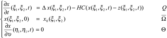
The notion of regional analysis was extended by El Jai and Zerrik et al. [8, 9]. This study motivated by certain concrete-real problems, in thermic, mechanic, environment [10, 11]. If a system defined on a domain Ω is represented as in the (Fig. 1), then we are interested in the regional state on ω or Г of the domain Ω.
The concept of asymptotic regional analysis was introduced recently by Al-Saphory and El Jai in [12, 13, 14], consists in studying the behavior of systems not in all the domain Ω but only on particular regions ω or Г of the domain. In this paper, we are only interested in the asymptotic regional boundary state on a region Г of the boundary ∂Ω. The purpose of this paper is to give some results related to the link between the Г-observer and the number of sensors, their locations, the geometrical domains and boundary conditions.
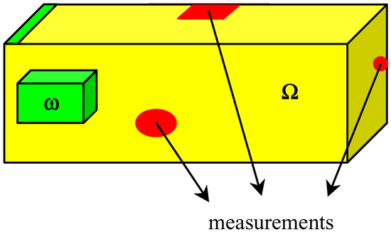
Figure 1.
Domain Ω, regions ω, Г and locations of measurements.
The paper is organized as follows. Section 2 concerns the formulation problem and preliminaries. Section 3, devotes to the introduction of Г-detectability problem. In section 4, we give some definitions and characterizations concerns Г-observer and strategic sensors. We show that there exists a counter-example of the case Г-observer which is not observer, in the whole domaine. In the last section, we illustrate applications with various situations of sensor locations and we characterize such a regional boundary observer to a diffusion system.
2. Problem Statement
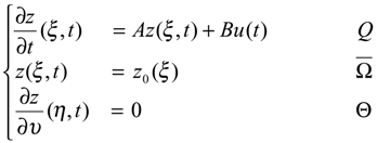
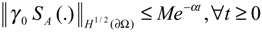
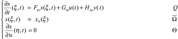
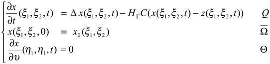
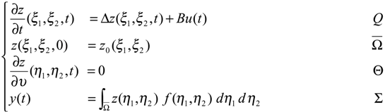
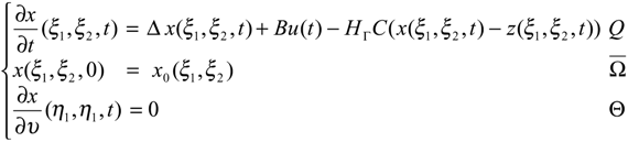
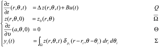
Let Ω be a regular, bounded and open set of Rn, with smooth boundary ∂Ω and Г be a nonempty given subregion of ∂Ω, with positive measurement. We denote Q = Ω × ]0,∞[ and Θ = ∂Ω × ]0,∞[. We consider the system described by the following parabolic equation
 with the output function
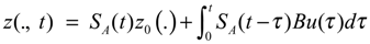
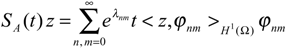
and we assume that Z, U, O be separable Hilbert spaces where Z is the state space, U the control space and O the observation space. Usually we consider Z = H1 (Ω), U = L2 (0,∞, Rp) and O = L2 (0,∞, Rq) where p and q hold for the number of actuators and sensors. A is a second order linear differential operator which generates a strongly continuous semi-group (SA (t)) t≥0 on Z and is selfadjoint with compact resolvent. The operators B∈L (Rp, Z) and C ∈L (Z, Rq) depend on the structure of actuators and sensors [7]. Under the given assumptions, the system (2.1) has an unique solution given by
with the output function
and we assume that Z, U, O be separable Hilbert spaces where Z is the state space, U the control space and O the observation space. Usually we consider Z = H1 (Ω), U = L2 (0,∞, Rp) and O = L2 (0,∞, Rq) where p and q hold for the number of actuators and sensors. A is a second order linear differential operator which generates a strongly continuous semi-group (SA (t)) t≥0 on Z and is selfadjoint with compact resolvent. The operators B∈L (Rp, Z) and C ∈L (Z, Rq) depend on the structure of actuators and sensors [7]. Under the given assumptions, the system (2.1) has an unique solution given by
 The measurements can be obtained by the use of zone, pointwise or lines sensors which may be located in Ω (or ∂Ω) [7].
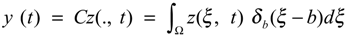
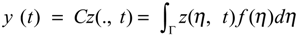
y(., t) = Cz(., t)
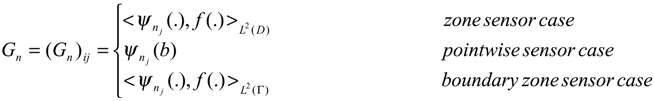
- Let us recall that a sensor by any couple (D, f) where D denote closed subsets of , which is spatial support of sensor and f ∈ L2 (D) defines the spatial distribution of measurement on D. According to the choice of the parameters D and f, we have various types of sensors. A sensors may be a zone types when D ⊂ Ω. The output function (2.2) can be written in the formy (t) = Cz(., t) = ∫D z(ξ, t) f (ξ)dξ
A sensor may also be a point when D = {b} and f = δ(. - b) where δ is the Dirac mass concentrated in b. Then, the output function (2.2) may be given by the form
In the case of boundary zone sensor, we consider D = Γ with Γ ⊂ ∂Ω and f ∈L 2 (Γ). The output function (2.2) can then be written in the form
The operator C is unbounded and some precautions must be taken in [7, 15].
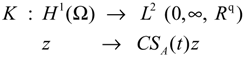
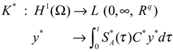
- The operator K defined byand in the case of internal zone sensors is, linear and bounded with an adjoint
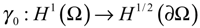
- The trace operator of order zerois linear, surjective and continuous with adjoint denoted by γ0*
- Consider a subdomain Γ of ∂Ω and let χΓ be the function defined bywhere z|Γ is the restriction of the state z to Γ. We denote by the adjoint of χΓ.
- Let χω be the function defined bywhere z|Γ is the restriction of the state z to ω.
- The operator TΓ : H1(Ω) → H1/2(Γ) is given by

Recalling some definitions concern the notion of Γ-observability as in [9, 16] :
- The autonomous system associated to (2.1)-(2.2) is said to be exactly (respectively weakly) Γ-observable if :

- The suite (Di, fi)1≤i≤q of sensors is said to be Γ-strategic if the system (2.1) together with the output function (2.2) is weakly Γ-observable. For the dual results concerning the actuators structures [17].
3. Regional boundary detectability
The main reason for introducing Γ-detectability is, the possibility to construct an Γ-estimator for the current state of the original system. This concept is extended by Al-Saphory and El Jai in [13]. For this objective we recall some definitions concern this concept :
- The system (2.1) is said to be ∂Ω-stable, if the operator A generates a semi-group which is stable on the space H1/2 (∂Ω). It is easy to see that the system (2.1) is ∂Ω-stable, if and only if, for some positive constants M and α, we have
If (SA(t))t≥0 is stable semi-group H 1/2(∂Ω), then for all z0 ∈H1 (Ω), the solution of the associated autonomous system satisfies

- The system (2.1) together with the output (2.2) is said to be ∂Ω-detectable, if there exists an operator H∂Ω: Rq → H1/2(∂Ω) such that (A – H∂ΩC) generates a strongly continuous semi-group (SH∂Ω (t))t≥0 which is stable on H1/2 (∂Ω).
- If a system is ∂Ω-detectable, then it is possible to construct an asymptotic ∂Ω-observer for the original system. If we consider the system
Remark 3.1.
In this paper, we only need the relation (3.1) to be true on a given subregion Γ of the region ∂Ω
 we may refer to this as Γ-stability.
- The system (2.1) is said to be Γ-stable, if the operator A generates a semi-group which is stable on H1/2 (Γ).
- The system (2.1)-(2.2) is said to be Γ-detectable if there exists an operator HΓ: Rq → H1/2(Γ) such that (A − HΓC) generates a strongly continuous semi-group (SHΓ(t))t≥0 which is stable on H1/2 (Γ).
For more detail [18]. However, one can easily have the following results :
Corollary 3.2.
If the system (2.1) together with output function (2.2) is exactly Γ-observable, then it is Γ-detectable.
This result leads to:

Thus, the notion of Γ-detectability is a weaker property than the exact Γ-observability as in (Ref. [16].
4. Asymptotic Γ-observer and strategic sensors
In this section, we propose an approach which allows to determinate a regional asymptotic estimator of z(ξ,t) on Γ, based on the internal asymptotic Γ-observer. This method need some definitions concern regional observer as in [11].
4.1. Definitions and characterizations
- Consider the system (2.1) - (2.2) together with the dynamical systemwhere Fω generates a strongly continuous semi-group (SFω(t))t≥0 which is stable on X = H1 (ω), i.e. :
 and Gω∈L(Rp, H1 (ω)) and Hω ∈L(Rq, H1 (ω)). The system (4.1) defines an asymptotic ω-estimator for χωT(ξ,t) where z(ξ,t) is a solution of the system (2.1) - (2.2) if and χωT maps D(A) into D(Fω) where x(ξ, t) is the solution of the system (4.1).
- The system (4.1) specifies an ω-observer for the system (2.1) - (2.2) if the following conditions hold:
- There exists Mω ∈ L(Rq, L2 (ω)) and Nω ∈ L(L2 (ω)) such that MωC + NωχωT = Iω.
- χωTA + FωχωT = GωC and Hω=χωTB.
- The system (4.1) defines an asymptotic ω-estimator for χωT (ξ,t).
- The system (4.1) is said to be an identity ω-observer for the system (2.1) - (2.2) if and Z = X.
- The system (4.1) is said to be a reduced-order ω-observer for the system (2.1) - (2.2) if Z = O ⊕X.
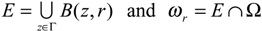
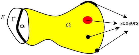 Figure 2. The considered domain Ω and the subregion ωr.
 - The boundary regional observer in Γ may be seen as internal regional observer in ω if we consider the following transformations. Let ℜ be the continuous linear extension operator [19] ℜ: H1/2 (∂ Ω) → H1 (Ω) such that

- Let r>0 is an arbitrary and sufficiently small real and let the setswhere B(z, r) is the ball of radius r centered in z(ξ,t) and where Γ is a part of (Fig. 2).
Proposition 4.1.
If the system (2.1) - (2.2) is exactly (respectively weakly) -observable, then it is exactly (respectively weakly) Γ-observable (see [9]).
From this result, we can deduce the following proposition :
Proposition 4.2.
The dynamical system (4.1) is Luenberger -observer for the system (2.1) - (2.2), then it is Luenberger Γ-observer.
Proof:
Let x(ξ, t) ∈H1/2 (Γ) and (ξ, t) its extension to H1/2 (∂Ω) using (4.3) and trace theorem, there exists ℜ(ξ, t)∈ H1 (Ω) with a bounded support such that
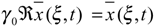 Since the system (4.1) is regional observer on so we can deduce that :
The system (4.1) is regional observer on ωr, there exists a dynamical system with x(ξ,t) ∈ X such that
 then we have
The equations (2.2) and (4.5) allow
 and there exist two linear bounded operators R and S satisfy the relation
There exists an operator is regionally stable on , then it is regionally stable on Γ [18]. Finally the system (4.1) is a regional boundary observer on Γ. ■
4.2 Sufficient condition for Γ-observer
As in (Refs. [7,18]), we develop a characterized result that links the Γ-observer and strategic sensors and we give a sufficient condition for Γ-observer. For that purpose, we assume that there exists a complete set of eigenfunctions ϕn of A in H1 (Ω), associated to the eigenvalues λn with a multiplicity sn and suppose that the functions ψn defined by ψn = χΓγ0ϕn(ξ), is a complete set in H1/2 (Γ). If the system (2.1) has J unstable modes, then we have the following theorem.
Theorem 4.3.
Suppose that there are q zone sensors (Di, fi)1≤i≤q and the spectrum of A contains J eigenvalues with non-negative real parts. If the following conditions are satisfied :
- q > s
- rank Gn = rn, ∀n, n = 1,..., J withwhere sup sn = s < ∞ and j = 1,..., sn. Then the dynamical system
 is Γ-observer for the system (2.1) - (2.2), i.e. .
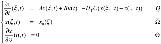
Proof :
The proof is limited to the case of zone sensors in the following stapes :
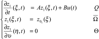
Step 1. Under the assumptions of section 2, the system (2.1) can be decomposed by the projections P and I - P on two parts, unstable and stable. The state vector may be given by where z1(ξ,t) is the state component of the unstable part of the system (2.1), may be written in the form
 and z2 (ξ,t) is the component state of the stable part of the system (2.1) given by
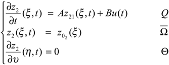
The operator A1 is represented by a matrix of order () given

Step 2. The condition (2) of this theorem, allows that the suite (Di, fi)1≤i≤q of sensors is Γ-strategic, the subsystem (4.7) is weakly Γ-observable [16] and since it is finite dimensional, then it is exactly Γ-observable. Therefore it is Γ-detectable, and hence there exists an operator such that (A1 −c) which is satisfied the following :
 and then we have
Since the semi-group generated by the operator A2 is stable on H1/2 (Γ), then there exist , > 0 such that
 and therefore ║z(ξ, t)║H1/2(Γ) → 0 when t → ∞. Finally, the system (2.1) - (2.2) is Γ-detectable.
Step 3. Let e(ξ,t) = z(ξ,t) − x(ξ,t) where x(ξ,t) is the solution of the system (4.6). Deriving the above equation and using the equations (2.1) and (4.6), we obtain
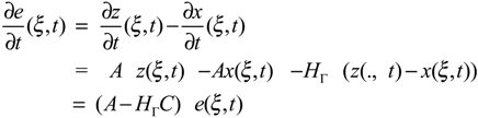
Since the system (2.1) - (2.2) is Γ-detectable, there exists an operator HΓ ∈ L(Rq, H1/2 (Γ)), such that the operator (A − HΓC), generates a stable, strongly continuous semi-group (SHΓ(t))t≥0 on the space H1/2 (Γ) which is satisfied the following relations :

Finally, we have
 with e0 (ξ,t) =z0 (ξ,t) − x0 (ξ,t) and therefore
 Thus, the dynamical system (4.6) a Γ-observer for the system (2.1) - (2.2). ■
Remark 4.4.
From theorem 4.3., we can deduce the following statements :
- A dynamical system which is an ∂Ω -observer is Γ-observer.
- If a system is Γ-observer, then it is Γ1 -observer in every subset Γ1 of Γ, but the converse is not true. This may be proven in the following example:
Example 4.5.
Consider a two-dimensional system described by the diffusion equation
 where Ω=]0,1[×]0,1[. The operator A = Δ generates a strongly continuous semi-group (SA(t))t≥0 on the Hilbert space H1 (Ω) given by
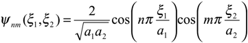
 where λnm = −(n2 + m2)π2, ϕnm(ξ1, ξ2) = 2anm cos(nπξ1) cos(mπξ2) and 2anm = (1 −λnm)−1/2.
Consider the dynamical system
 where H ∈ L(Rq, Z), Z is a Hilbert space and C :H1 () → Rq is a linear operator. Consider the boundary sensor (Γ0, f) defined by Γ0 ={0} × ]0,1[ and f (η1,η2) = cosπη2. Thus, the output function can be written by
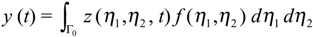
If the state z0 is defined in Ω by z0 (ξ1, ξ2) = cos(πξ1)cos(2πξ2), then the system (4.9) - (4.11) is not weakly observable in Ω, i.e. the sensor (Γ0, f) is not strategic and therefore the system (4.9) - (4.11) is not detectable in Ω. Thus, the dynamical system (4.10) is not observer for the system (4.9) - (4.11) (see [6]). Here, we consider the region Γ = ]0,1[×{0} ⊂∂Ω (Fig. 3) and the dynamical system
 where H ∈L(Rq, H1/2 (Γ)) . In this case, the system (4.9) - (4.11) is weakly observable in Γ and the sensor (Γ0, f) is Γ-strategic [9]. Thus, the system (4.9) - (4.11) is Γ-detectable [13]. Finally the dynamical system(4.9) is Γ-observer for the system (4.9) - (4.11) [18].
Figure 3.
Domain Ω, region Γ and location Γ0 of zone sensor.
5. Application to sensors structures
In this section, we consider the distributed diffusion systems defined on Ω =]0,a1[×]0,a2[. We explore various results related to different types of measurements, domains and boundary conditions.
5.1 Case of a zone sensor
We study the following cases :
5.1.1 Rectangular domain
In this case, the system (2.1) - (2.2) is given by
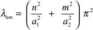
 where is the location of zone sensor and above system represent the heat-conduction problem (see Ref. [20]). Let Γ = {a1}×]0, a2[ be a region of on ]0,a1[×]0,a2[ The eigenfunctions and the eigenvalues are given by
 and
and
If , then the multiplicity of snm = 1 and one sensor can be guaranteed Γ -strategic sensor (see [21]). The dynamical system (4.6) may be given by
Let the measurement support is rectangular with D = [ξ1 − l1, ξ1 + l1] × [ξ2 − L2, ξ2 + L2] ∈ Ω.
If f1 is symmetric about ξ1 = ξ01 and f2 is symmetric with respect to ξ2 = ξ02, then we have the following result :
Corollary 5.1.
The dynamical system (5.4) is Γ-observer for the system (5.1) if nξ01 / a1 and mξ02 / a2 ∉ N for every n, m =1,..., J.
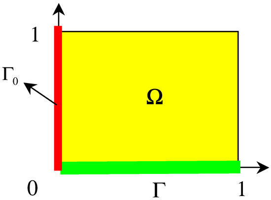
In the case where Γ ⊂ ∂Ω and f ⊂ L2 (Γ), the sensor (D, f) may be located on the boundary in Γ0 = [η01 − l, η01 + l]×{ a2 } then we have :
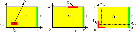
Figure 4.
Domain Ω, region Γ and locations D, Γ0, of zone sensor.
Corollary 5.1.
- One side case : Suppose that the sensor (D, f) is located on Γ0 =[η01 − l, η01 + l] × { a2 } ⊂ ∂Ω and f is symmetric with respect to η1 = η01, then the dynamical system (5.4) is Γ-observer for the system (5.1) if n η01 / a1 ∉N for every n, m =1,..., J.
- Two side case : Suppose that the sensor (D, f) is located on and is symmetric with respect to η1 = η01 and the function is symmetric with respect to η2 = η02, then the dynamical system (5.4) is Γ-observer for the system (5.1) if n η01 / a1 and mη02 / a2 ∉N for every n, m = 1,..., J.
5.1.2 Disk domain
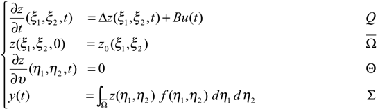
The system (5.1) may be given by the following form
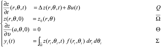 where 0 < θi< 2π, Ω = D(0, a), r = a > 0 and Θ = θ ∈[0, 2π], t > 0 are defined as in (Fig. 5).
Let the eigenfunctions and eigenvalues concerning the region Γ = D(a, θi)2≤i≤q of ∂Ω with θi ∈ [0, 2π] are defined by
 where βnm are the zeros of the Bessel functions Jn and
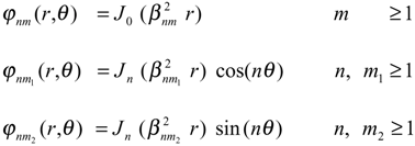
 with multiplicity snm = 2 for all nm ≠ 0 and snm = 1 for all nm = 0. In this case, the Γ–strategic sensor is required at least two zone sensors (Di,fi)2≤i≤q where Di =(ri,θi)2≤i≤q (see [6]). The dynamical system (5.4) can be written by
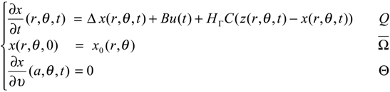
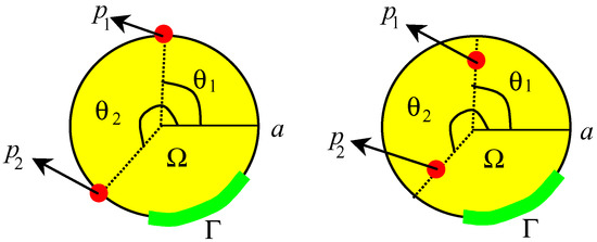
Figure 5.
Domain Ω, region Γ and locations p1, p2 of internal (boundary) zone sensors.
If fi and Di are symmetric with respect to θ = θi, for all 2 ≤i ≤ q, then we have :
Corollary 5.3.
The dynamical system (5.8) is Γ-observer for the system (5.5) if n(θ1 − θ2)/π ∉ N for every n, n = 1,..., J.
When the sensors (Γi,fi)2≤i≤q are located on ∂Ω and the function f|Γi is symmetric with respect to θ = θi, 2 ≤ i ≤ q as in (Fig. 5). So, we have.
Corollary 5.4.
The dynamical system (5.8) is Γ-observer for the system (5.5) if n(θ1 − θ2) /π ∉ N for every n, n =1,..., J.
5.2 Case a pointwise sensor
In this subsection, we consider the following cases :
5.2.1 The domain Ω =]0,a1[×]0,a2[
Now the system (5.5) is given by the form
If b = (b1,b2) ∈∂Ω then, we have :
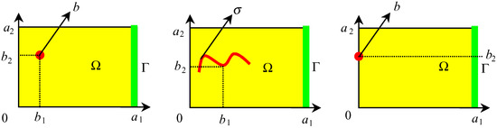
Figure 6.
Rectangular domain, region Γ and locations b, σ of pointwise sensors.
Corollary 5.5.
- Internal case : If nb1 / a1 and mb2 / a2 ∉N for every n, m = 1,..., J, then the dynamical system (5.4) is Γ-observer for the system (5.9).
- Filament case : Suppose that the observation is given by the filament sensor where σ = Im(γ) is symmetric with respect to the line b = (b1,b2), if nb1 / a1 and mb2 / a2 ∉N for every n, m = 1,..., J, the dynamical system (5.4) is Γ-observer for the system (5.9).
- Boundary case : If mb2 / a2 ∉N for every m = 1,..., J, then the dynamical system (5.4) is Γ- observer for the system (5.9).
5.2.2 The domain Ω = D(0,a)
The system (5.5) may be given by the following form
 Where 0 ≤ θi ≤ 2π. The sensors may be located in p1 =(r1,θ1) and p2 =(r2,θ2) ∈ Ω (or in pi = (a,θi) ∈Ω) (Fig. 7).
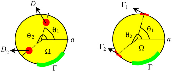
Figure 7.
Disc domain, region Γ and locations p1, p2 of internal (boundary) pointwise sensors.
Corollary 5.6.
- If the sensors (pi,δpi)2≤i≤q are located in pi =(ri,θi) and n(θ1 − θ2)/π ∉ N for every n, n =1,..., J, then the dynamical system (5.8) is Γ-observer for the system (5.10).
- If the sensors (pi,δpi) are located in pi =(a,θi) 2≤i≤q and n(θ1 − θ2)/π ∉ N for every n, n =1,..., J, then the dynamical system (5.8) is Γ-observer for the system (5.10).
6. Conclusion
The concept studied in this paper is related to the case of identity Γ-observer in connection with the sensors structure. For this class of parabolic distributed parameter systems, many interesting results concerning the choice of the sensor are explored and illustrated in specific situations of the domain. In similar way, we can characterize the general case (reduced-order) Γ-observer by sensors structure. An important extension of these results, related to the problem of regional boundary gradient observer, in connection with the structure of sensors; is under consideration.
References
- Luenberger, D. Observers for multi-variable systems. IEEE Transactions on Automatics Control 1966, 11, 190–197. [Google Scholar] [CrossRef]
- Gressang, R.; Lamont, G. B. Observers for systems characterized by semi-groups. IEEE Transactions on Automatics Control 1975, 20, 523–528. [Google Scholar] [CrossRef]
- Fujii, N.; Hirai, M. A finite-dimensional asymptotic observer for a class of distributed parameter systems. International Journal of Control 1980, 32, 951–961. [Google Scholar] [CrossRef]
- Hou, M.; Muller, P.C. Design of observers for linear systems with unknown inputs. IEEE Transactions Automatic Control 1992, 37, 871–875. [Google Scholar] [CrossRef]
- Curtain, R. F.; Zwart, H. J. Introduction to infinite dimensional linear theory systems; Springer-Verlag: New York, 1995. [Google Scholar]
- El Jai, A.; Pritchard, A. J. Sensors and actuators in distributed parameter systems. International Journal of Control 1987, 46, 1139–1153. [Google Scholar] [CrossRef]
- El Jai, A.; Pritchard, A. J. Sensors and controls in the analysis of distributed systems; Ellis Horwood series in Mathematics and its Applications; Wiley: New York, 1988. [Google Scholar]
- El Jai, A.; Simon, M. C.; Zerrik, E. Regional observability and sensor structures. Sensors and Actuators 1993, 39, 95–102. [Google Scholar] [CrossRef]
- Zerrik, E.; Badraoui, L.; El Jai, A. Sensors and regional boundary state reconstruction of parabolic systems. Sensors and Actuators 1999, 75, 102–117. [Google Scholar] [CrossRef]
- El Jai, A.; Zerrik, E.; Simon, M. C.; Amouroux, M. Regional observability of a thermal process. IEEE Transactions on Automatic Control 1995, 40, 518–521. [Google Scholar] [CrossRef]
- Al-Saphory, R.; El Jai, A. Sensors and asymptotic ω-observer for distributed diffusion systems. Sensors 2001, 1, 161–182. [Google Scholar] [CrossRef]
- Al-Saphory, R.; El Jai, A. Sensors structures and regional detectability of parabolic distributed systems. Sensors and Actuators 2001, 29, 163–171. [Google Scholar] [CrossRef]
- Al-Saphory, R.; El Jai, A. Sensors characterizations for regional boundary detectability of distributed parameter systems. Sensors and Actuators 2001, 94, 1–10. [Google Scholar] [CrossRef]
- Al-Saphory, R.; El Jai, A. Asymptotic regional state reconstruction. International Journal of Systems Science 2002. to appear. [Google Scholar] [CrossRef]
- Curtain, R. F. Finite dimensional compensators for parabolic distributed systems with unbounded control and observation. SIAM J. Control and Optimisation 1984, 22, 255–275. [Google Scholar] [CrossRef]
- Zerrik, E.; Badraoui, L. Sensors characterization for regional boundary observability. International Journal of Applied Mathematics and Computer Science 2000, 10, 345–356. [Google Scholar]
- Zerrik, E.; Boutoulout, L.; El Jai, A. Actuators and regional boundary controllability of parabolic systems. International Journal of Systems Science 2000, 31, 73–82. [Google Scholar] [CrossRef]
- Al-Saphory, R. Asymptotic regional analysis for a class of distributed parameter systemes. Ph.D. thesis, University of Perpignan, France, 2001. [Google Scholar]
- Dautray, R.; Lions, J.L. Analyse mathématique et calcul numérique pour les sciences et les techniques; série scientifique 8; Masson: Paris, 1984. [Google Scholar]
- Kitamura, S.; Sakairi, S.; Nishimura, M. Observer for distributed-parameter diffusion systems. Electrical engineering in Japan 1972, 92, 142–149. [Google Scholar] [CrossRef]
- El Jai, A.; El Yacoubi, S. On the number of actuators in parabolic system. International Journal of Applied Mathematics and Computer Science 1993, 3, 673–686. [Google Scholar]
- Sample Availability: Available from the authors.
© 2002 by MDPI (http://www.mdpi.net). Reproduction is permitted for noncommercial purposes.