1. Introduction
Detecting and estimating the target position underwater have many important applications including underwater localization, deep sea exploration and rescue missions in catastrophic conditions. However, underwater localization still remains a challenge in robotics [
1,
2,
3]. In the last few decades, the acoustic-based locating method has played a main role in underwater localization [
4,
5,
6]. The echolocation obtained by sonar is problematic because the varying temperature and density, Doppler effect and background noise might cause interferences to the signal [
7,
8]. The light- or map-based underwater localization method is restricted by the transparency of water, which cannot work in a dark or turbid environment [
9]. To overcome these drawbacks, in fact, nature has already discovered an original sense to adapt well to this situation: the electric sense [
1]. The electric fish has an electric organ of discharge located at the base of its tail, which can help it detect and locate the target in a dark and turbid environment. The electric organ of discharge generates a dipolar-shaped electric field around the fish, which can be distorted by the surrounding objects. Then, the fish “measures” the distortions of the electric field by using the electro-receptors distributed along its body and uses its brain to get an image of its surroundings [
10,
11]. This means that understanding and imitating the electric sense with technology would offer the opportunity to enhance the target detecting and locating abilities of underwater robots.
In this perspective, in [
12], the authors set up an experiment by using four-point electrodes that are placed at the apexes of a rhombus in a rigid moving frame driven by a robot. In this system, two electrodes that are situated at the opposite apexes of the lozenge are polarized in voltage and play the role of the electric organ of discharge, while the other two opposite electrodes play the role of receivers. Rasnow [
13] first applied a small sphere perturbation formula in a uniform electric field, which is still very popular in the latest electro-location literature [
10,
14,
15,
16]. However, in this theoretical model, the field near the target should be a uniform electric field, which means that the radius of spherical targets should be small. Thus, the surrounding field performs as the uniform electric field. In the works [
17], an artificial electrosensory array was designed to study the feasibility in underwater robots. The artificial electrosensory array was able to estimate the position of a plastic sphere with a diameter of 10 mm, when the plastic sphere was 12 mm away from the electrosensory array. Their distance estimation algorithm was realized based on the spatial distribution of the sensor measurements [
18]. In Lebastard’s work [
3,
19], a bio-inspired method has been proposed to improve the localization performance on the basis of the unscented Kalman filter. In Peng’s work [
20], a finite element model (FEM) of underwater an active electrolocation system based on the coupling Cole–Cole model and Maxwell theory was built. However, in both Lebastard’s and Peng’s electro-location systems, the electrosensory array needs to move and measure the electric field while locating the target, which is not suitable for positioning a dangerous target in practice. In the work [
21], a MUSIC-type algorithm is proposed for locating small inclusions buried in a half-space by means of measuring the scattering amplitude at a fixed frequency in two-dimensional space. The locating method is based on far area theory. However, far area theory is not suitable for underwater target locating because the high frequency radiation wave cannot be transferred a long distance.
Considering the challenges of the underwater target localization, this paper proposes a novel solution for underwater locating based on the boundary element method (BEM) theory and mixed polarization multiple signal classification (MP-MUSIC) algorithm. In this method, we first use the BEM to accurately describe the induction field of the metallic target and insulator target with Poisson’s equation. Then, a UCA system is designed, which acts as the underwater target locating sensors. In these locating sensors, two electrodes act as the dipole source, while five electrodes situated at the equipotential points of the dipole source play the role of receivers. One of the five electrodes is set as the reference point, and hence, we can measure the voltage between the other four electrodes and the reference point. Since the five electrodes of the UCA system are situated at the equipotential points of the dipole source, they cannot receive the primary field of the dipole source. However, they can receive the induction field from the target. In the locating procedure, we introduce the mixed polarization MUSIC algorithm, which provides good performance and does not suffer from the problem of non-convexity [
22,
23]. Different from the other MUSIC algorithms for radar, such as root-MUSIC and beamspace MUSIC, MP-MUSIC could deal with signal polarization, which is suitable for underwater electro-location. The position of the target can be located via finding the minimum eigenvalue of the estimated gain matrix and the project matrix of the noise subspace by using the MP-MUSIC algorithm [
24]. We also propose a simplified locating model and introduce the Rasnow model and canonical MUSIC for comparison in this paper. The effectiveness of the proposed method is investigated and compared with the numerical model and simulation model. We also setup a physical experiment to verify the proposed locating method. The results show that the proposed algorithm is effective for underwater target locating.
3. Numerical Examples
In this section, we present a numerical example and a simulation model to illustrate the features of our proposed localization method. The conductivity of the locating area is
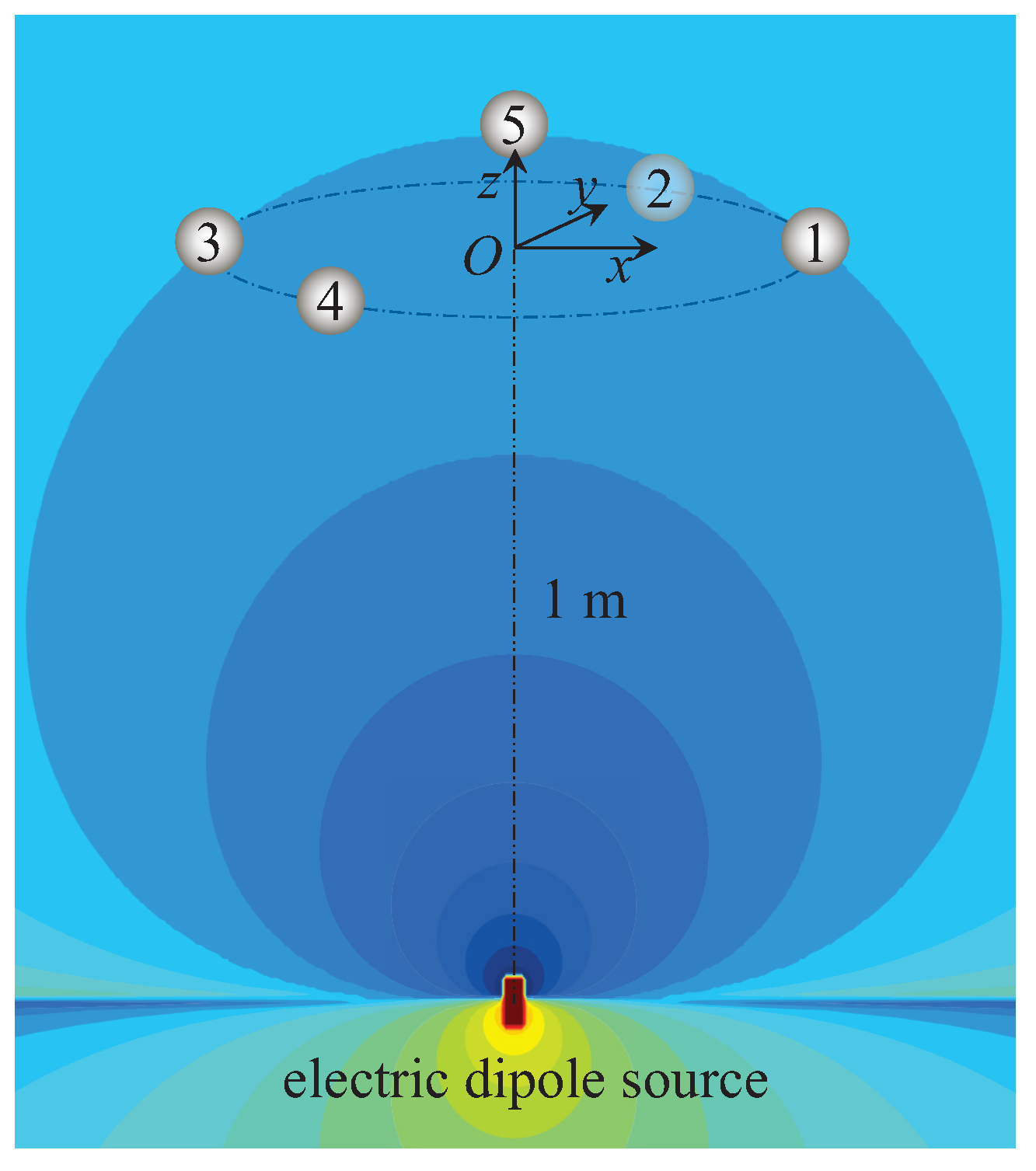
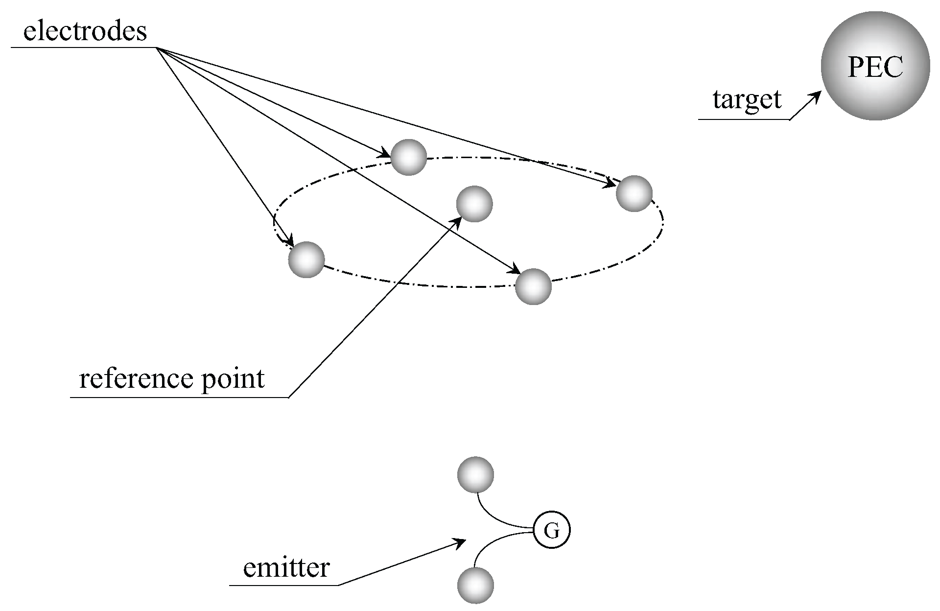
, which is the same as the seawater. A UCA system is designed, which consists of two parts. The first part is the emitter, which is an ideal electric dipole source. The electric dipole source is situated at
m with the dipole moment
along the
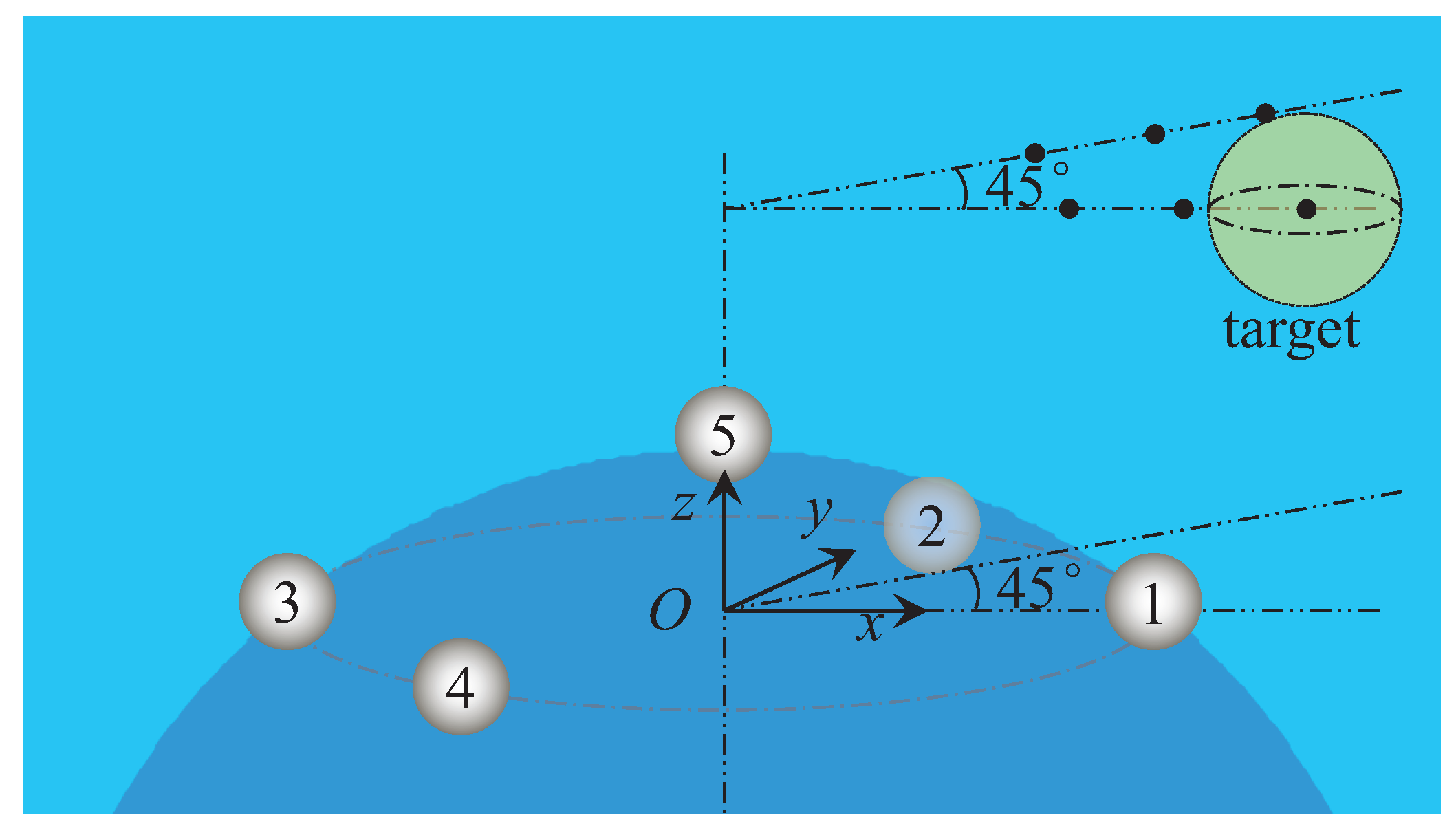
z-axis. The second part is the receptor, which is the ideal points in this simulation model. The electrodes positions in the UCA system are listed in
Table 1 and shown in
Figure 2. The electrodes Index Numbers 1–4 are uniformly distributed on a circle of radius
m, and the fifth electrode is set as the reference electrode. We define the output data of channel
k as the voltage between the
k-th electrode and the reference electrode,
. Additionally, the five electrodes are set at the equipotential points of the electric dipole source, which means that the voltage from channel
k should be zero when there is no target in the observation area. Then, a spherical target with a radius of
m is discretized into 3004 triangular patches. In this locating system, we hold the number of time samples constant at 200 for one locating operation, yielding
in (
40).
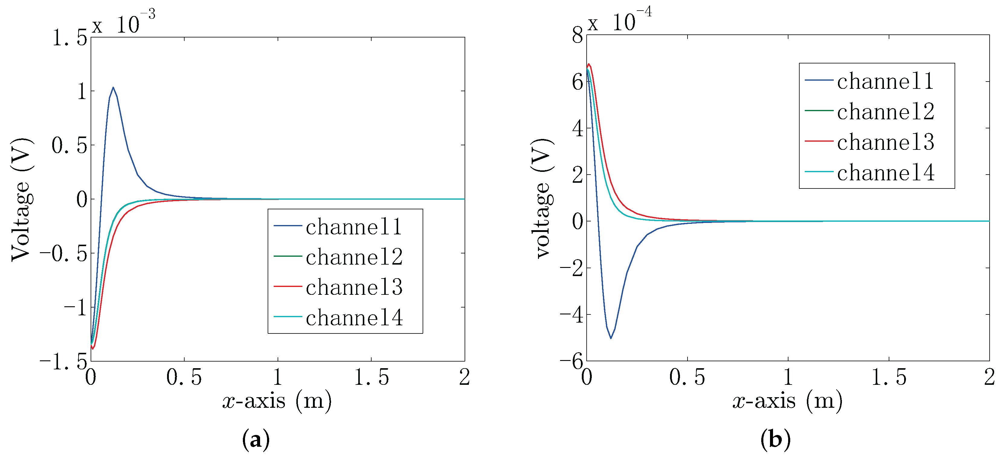
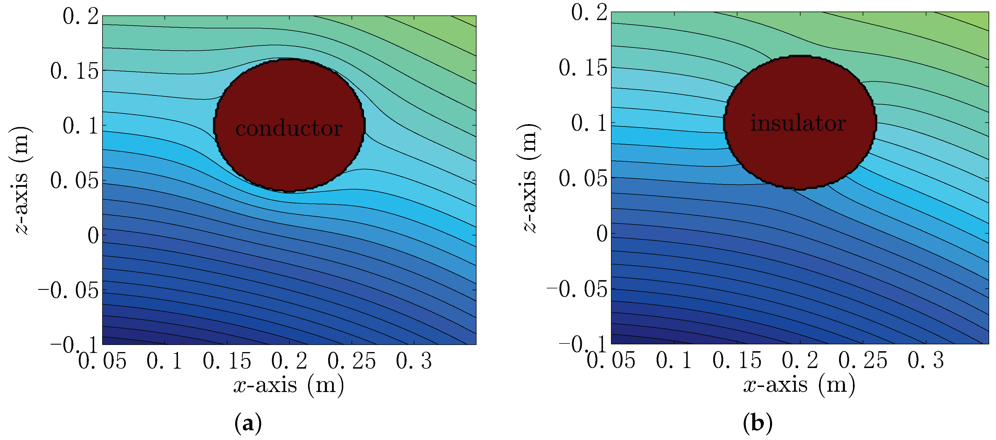
When the target is located near the UCA system, the voltage of each channel of the UCA system can be obtained.
Figure 3a shows the obtained voltage of each channel when the conductor target is set at position
.
Figure 3b shows the obtained voltage when the insulator target is set at position
. From
Figure 3, it can be seen that the voltage amplitude in Channel 1 has a different property from the other three channels. That is because the distance between the target and Electrode 1 decreases as
x increases when
, and it increases when
. Electrodes 2 and 4 are symmetric about the
x-axis, yielding that Channels 2 and 4 have the same voltage curves when the target is located on the
x-axis. The voltage of each channel contains the position information of the target, which allows the electric-locator to estimate the target position based on the BEM and MP-MUSIC algorithm.
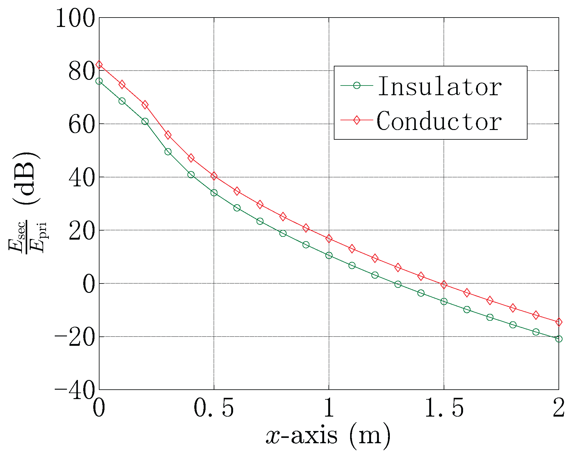
The proposed UCA system can reduce the influence of the electric dipole source.
Figure 4 shows the comparison between the magnitude of the primary energy generated by the emitter
and the secondary energy reflected by the spherical target
. From
Figure 4, it can be seen that
plays the main role when
m for the conductor target and
m for the insulator target, where the contribution of
can be neglected. However, for the conductor target, the
will not be neglected, when the target lies in
m. For the insulator target, the
will not be neglected, when the target lies in
m. In the practical scenario, the reference point is close to, but not at the equipotential point, which causes the primary energy
not to be zero. Moreover, the secondary energy
will decrease as the target gets far from the UCA, which results in the decrease of the ratio of
, where:
According to the measured voltage obtained from each channel of the proposed UCA system, the spectrum can be obtained, with which the electro-locator can estimate the position of the target. The additive white Gaussian noise is added to all measured voltage data, where the squared Frobenius norm of the noiseless signal matrix
is one hundred times that of the squared Frobenius norm of the noise matrix
. As a result, the signal-to-noise ratio (SNR) is 20 dB [
29,
30].
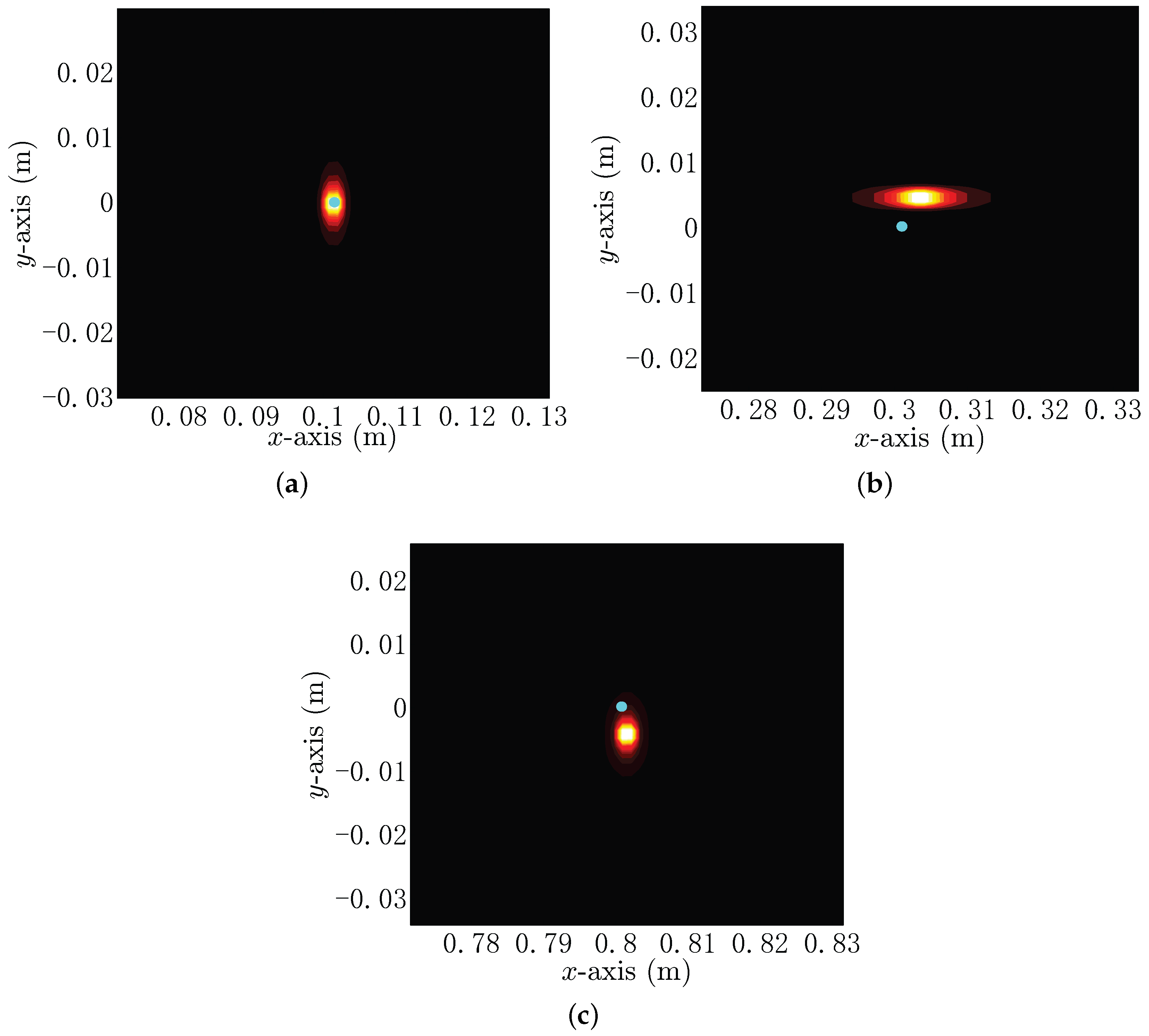
Figure 5 gives the spectrum images of an insulator with the radius of
m when it is situated at points
m,
m and
m, respectively. The real position of the target is marked with a blue point, and the highlighted spots in the spectrum images indicate the estimated positions of the target. The peaks of the spectrum images are
m,
m and
m, which are the estimated positions by the use of the proposed electro-locator. The corresponding location errors are
m,
m and
m, which shows that the proposed locating method can be applied in underwater target locating. Next, we will study the locating performance in detail.
In the practical situation, the noise can affect the locating performance. Generally, the noise power of each channel in the UCA system is constant. Thus, we add the additive white Gaussian noise to all measured voltage data, yielding the SNR of 20 dB, when the conductor target is located at
m. We refer to the noise as the background noise.
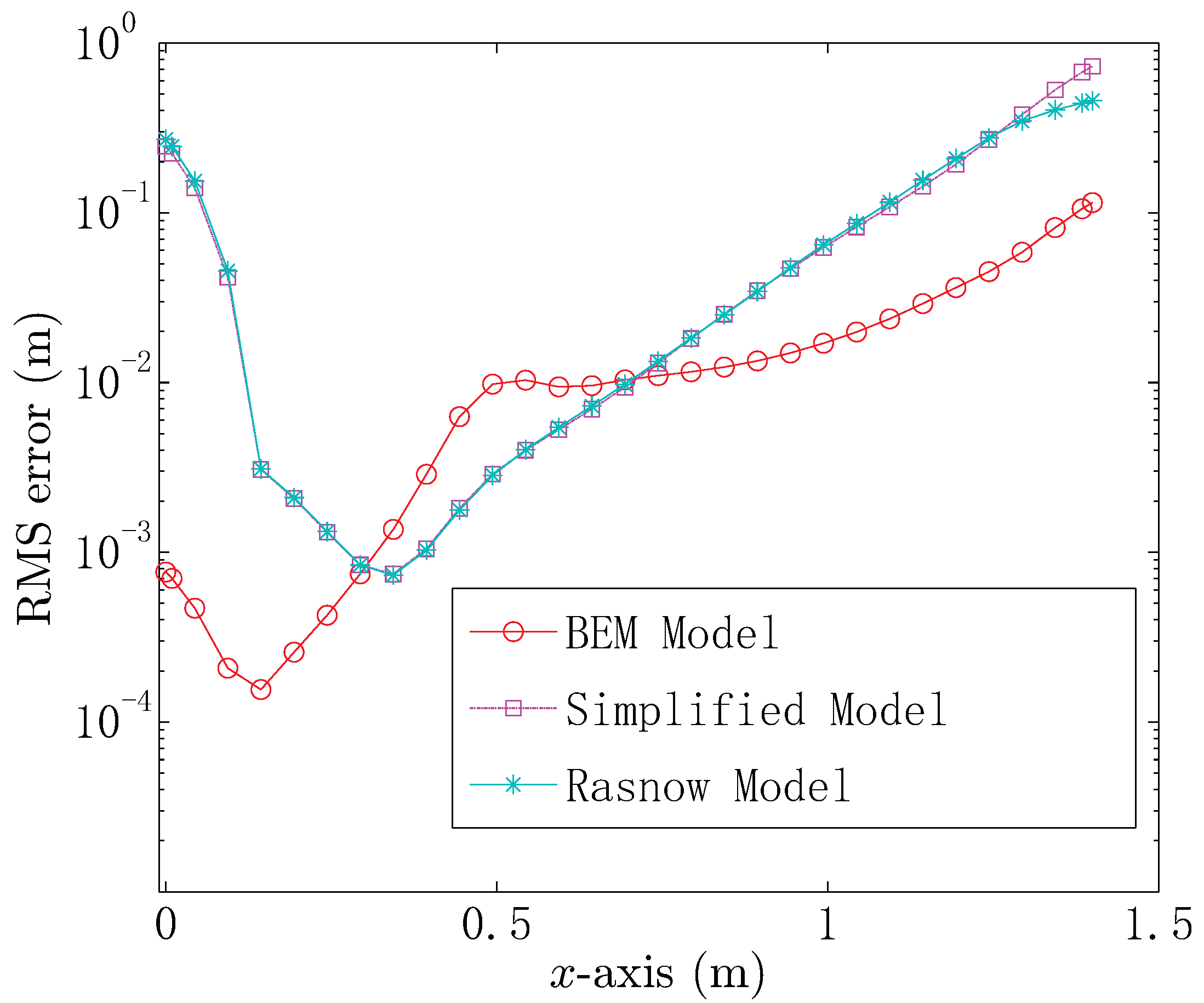
Figure 6 shows the root mean square (RMS) errors for locating the conductor target, which is situated at the continuous positions
m. From
Figure 6, it is obvious that the simplified model has the same locating performance as the Rasnow model, when
. The reason is that both the simplified model and the Rasnow model consider the spherical target as an equivalent electric dipole. It can also be seen that the RMS error of the three models first decreases as
x increases. The UCA system and the conductor target are both symmetrical structures, which means that the voltage data of the four channels in the UCA system will be similar as the target gets close to the
z-axis. As a result, the simplified model, Rasnow model and BEM model have lower locating accuracy, when the target gets close to the center of the UCA system. When the target gets far from the center of the UCA system, the localization method can give the voltage difference between each channel by using the three models, resulting in a decrease of the locating RMS error. However, the secondary energy will decrease when the target is getting far from the UCA system and the energy of the background noise remains constant. Thus, the RMS error increases when
for the simplified model and Rasnow model and
for the BEM model. It should be noted that the BEM model shows better locating performance compared with the simplified model and Rasnow model in most cases. However, the simplified model and Rasnow model provide better locating performance when
.
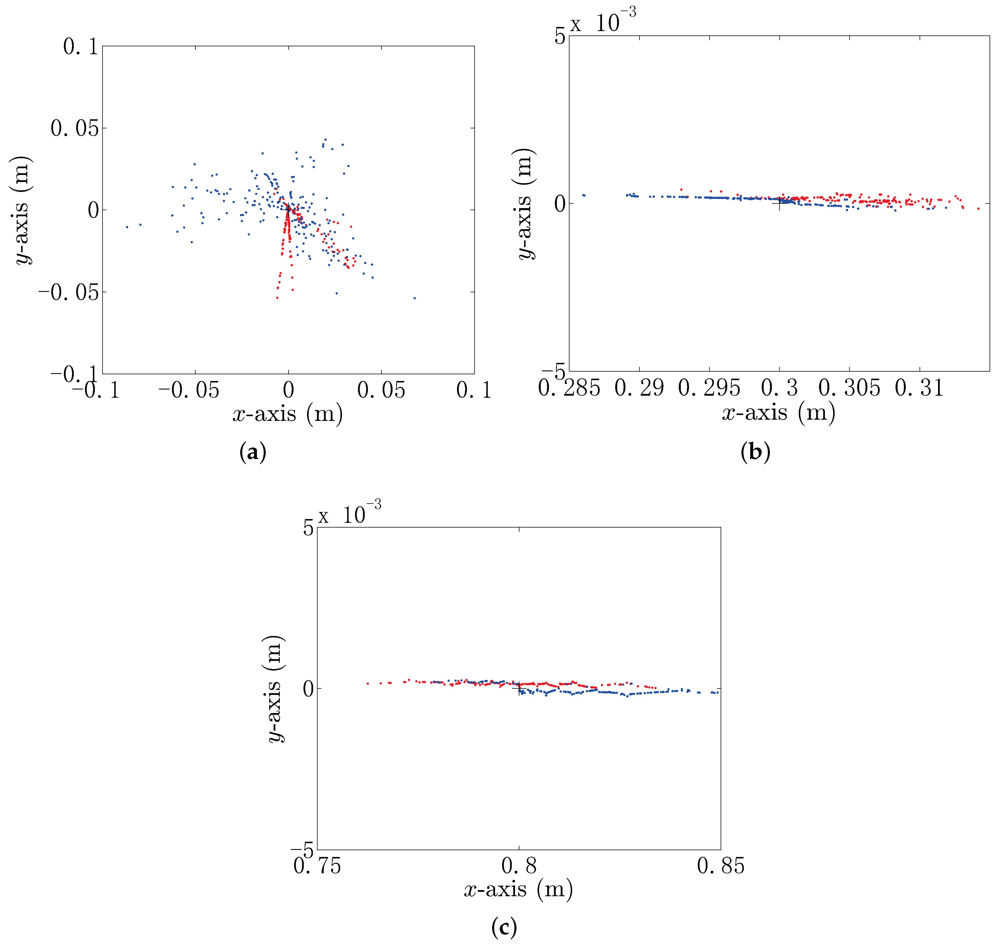
The locating results are obtained by the use of the BEM-based model and simplified model and compared under the same SNR.
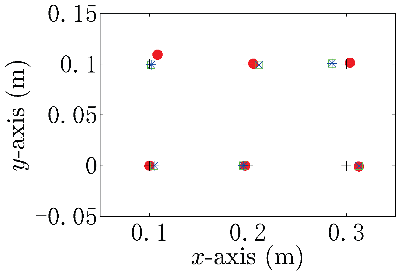
Figure 7 shows the 200-times independent locating operation by using the BEM model and the simplified model with
dB when the target is situated at
,
and
. The blue scatters in
Figure 7 are the estimated positions by using the simplified model, and the red ones are the estimated positions by using the BEM model. In
Figure 7, the average estimated positions by using the simplified model are
,
and
. The average estimated positions by using the BEM model are
,
and
. It can be seen from
Figure 7a that the distribution of the blue scatters is sparser than that of the red scatters, but not obviously, which means that the proposed localization methods have comparable localization performance, when the target gets close to the center of the UCA system. In
Figure 7b,c, we can see that the locating method based on the simplified model and BEM model provides better locating performance in the
y-direction.
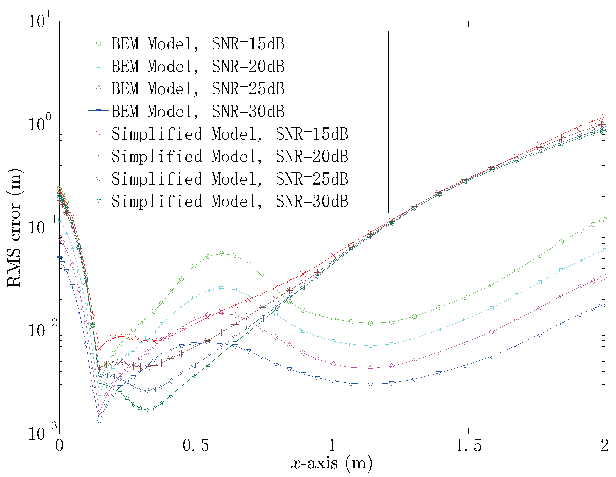
In order to evaluate the accuracy of the proposed localization method when the target is situated at the continuous positions
, the RMS errors of the estimated position by using the simplified model and BEM model at the same SNR are given and compared in
Figure 8 and
Table 2. For the simplified model, the RMS error curves are close to the others when
and
, which means that the RMS errors would not decrease obviously as the SNR increases. The RMS errors decrease significantly as the SNR increases by using the BEM model. Furthermore, the BEM model provides more accurate estimation of the position compared with the simplified model with the same SNR when
and
. It should be noted that the simplified model shows good locating performance when
. For example, when the target is located at
, the RMS errors are
m and
m by using the simplified model at 15 dB and 30 dB, respectively; whereas the RMS errors are
m and
m by using the BEM model.
The locating performance of the proposed UCA is investigated when the target is situated at different azimuths, which is shown in
Figure 9. Two azimuths with different distances
r from the center of the UCA are taken into consideration when the SNR is equal to 20 dB.
Table 3 shows the comparison results by using the canonical MUSIC and MP-MUSIC locating algorithm, when the azimuths are zero degrees (along the
direction) and 45 degrees (along the
direction). From
Table 3, we can see that the locating method based on the BEM model and MP-MUSIC provides a similar locating performance when the azimuths are zero degrees and 45 degrees. Additionally, the locating method based on the Rasnow model and MP-MUSIC also provides a similar locating performance when the azimuths are zero degrees and 45 degrees. However the locating error significantly increases when
m, compared to the BEM model with the MP-MUSIC algorithm. The BEM model and canonical MUSIC algorithm-based locating method is sensitive to the azimuth, providing high locating errors when the azimuth is 45 degrees. We can also see that the Rasnow model with the canonical MUSIC algorithm could hardly give satisfactory localization when the azimuth is 45 degrees, which indicates that the Rasnow model with the canonical MUSIC algorithm is not suitable for underwater target locating. The comparison results in
Table 3 indicate that the BEM model with the MP-MUSIC can satisfy the locating resolution well when the azimuth changes.
In this paper, the receptor of the UCA system consists of five electrodes, yielding four measurement channels. Theoretically, the reference point
and points on the circle
l:
are of the same potential, where
. We investigate the locating performance of the UCA system with
Q electrodes uniformly distributed on the circle
,
.
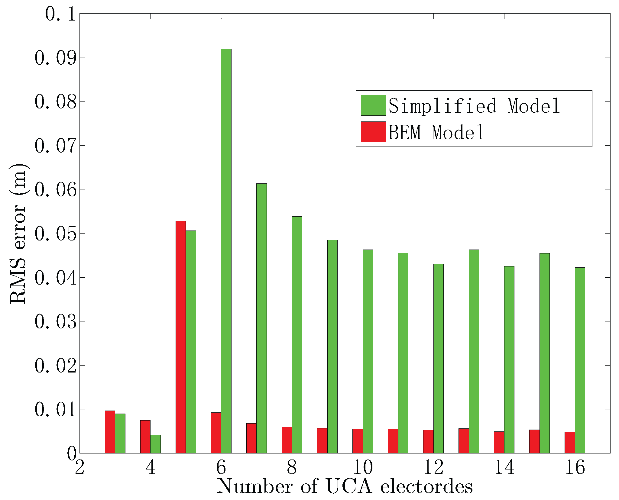
Figure 10 shows the RMS of the estimated position versus the number of electrodes by using the simplified model and BEM model, when the target is situated at
with
dB. From
Figure 10, we found that increasing the number of electrodes will not improve the locating accuracy significantly. It is obvious that the simplified model provides lower RMS errors compared with the BEM model when
and 5. However, the RMS errors are large when the number of electrodes
, and the RMS errors are about
m. The simplified model provides the best locating performance when the number of electrodes is four. For the BEM model, the RMS errors are stable as the number of electrodes increases when
and
. The BEM model shows the worst locating accuracy when the number of electrodes is taken as five and the RMS error is greater than
m. Thus, according to
Figure 10, the optimal number of electrodes in the UCA system for the BEM model and the simplified model is four.
In this section, a locating simulation scenario is proposed to analyze the performance of the proposed localization methods and the UCA system. The simulation results show that both the BEM model and simplified model provide acceptable locating accuracy, especially when , compared with the Rasnow model. However, the proposed locating models show unsatisfactory locating results when the target gets close to the center of the UCA system. The receptor of the UCA system is specially designed, which can only sense the induction field of the target and cannot sense the field from the emitter of the UCA system itself. We also find that the MP-MUSIC provides better locating performance than the canonical MUSIC algorithm when the target is located at different azimuths. It should be noted that increasing the number of receiving electrodes would not improve the locating accuracy significantly. On the contrary, increasing the number of receiving electrodes may result in performance degradation. For this locating scenario and the UCA system, the optimal number of the electrodes on the circle l is four. Additionally, the gain matrix of the simplified model is much simpler than the gain matrix of the BEM model. As a result, localization based on the simplified model would reduce the computational burden. In the required real-time scenario, the simplified model would provide more advantages.
5. Experiment
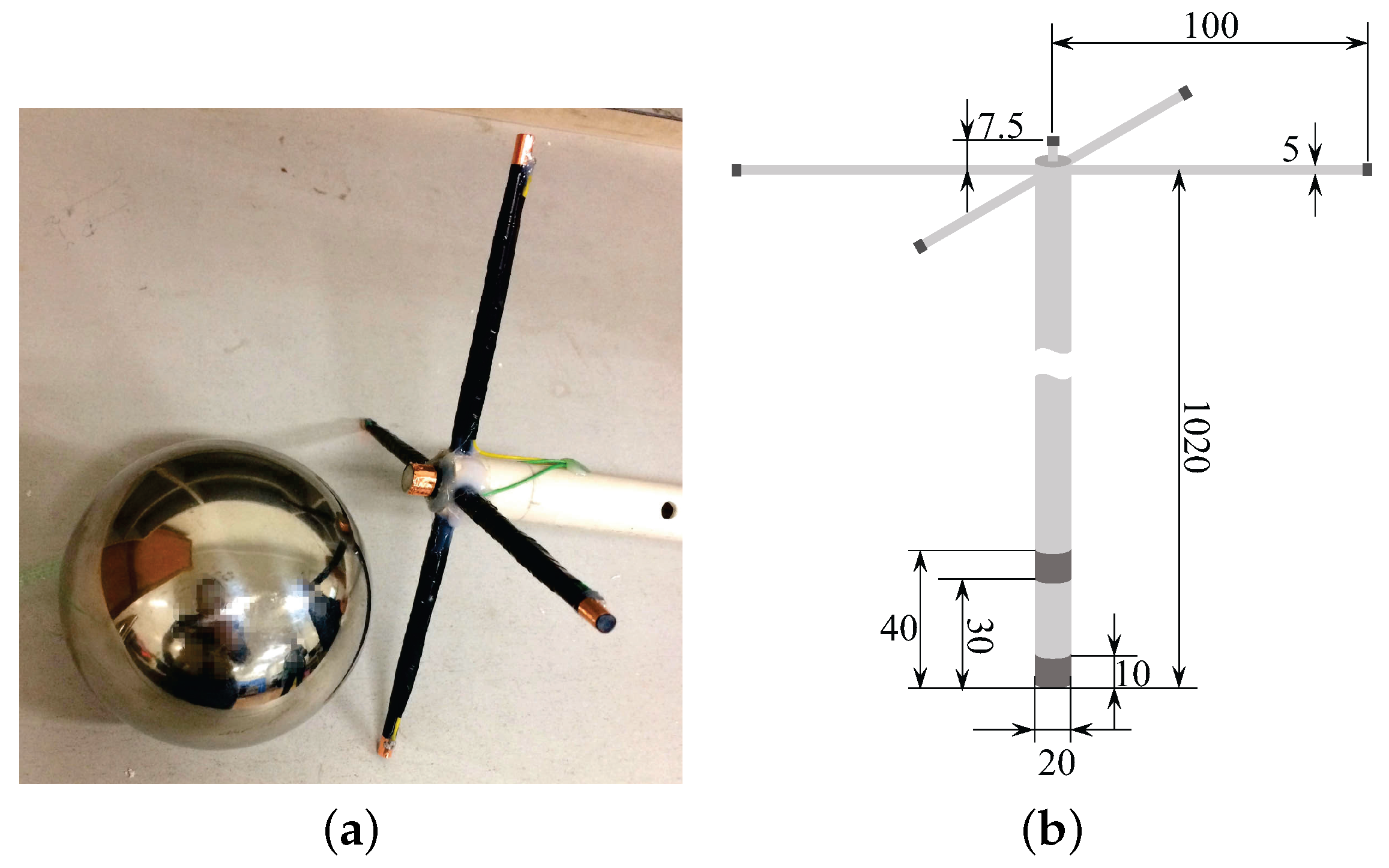
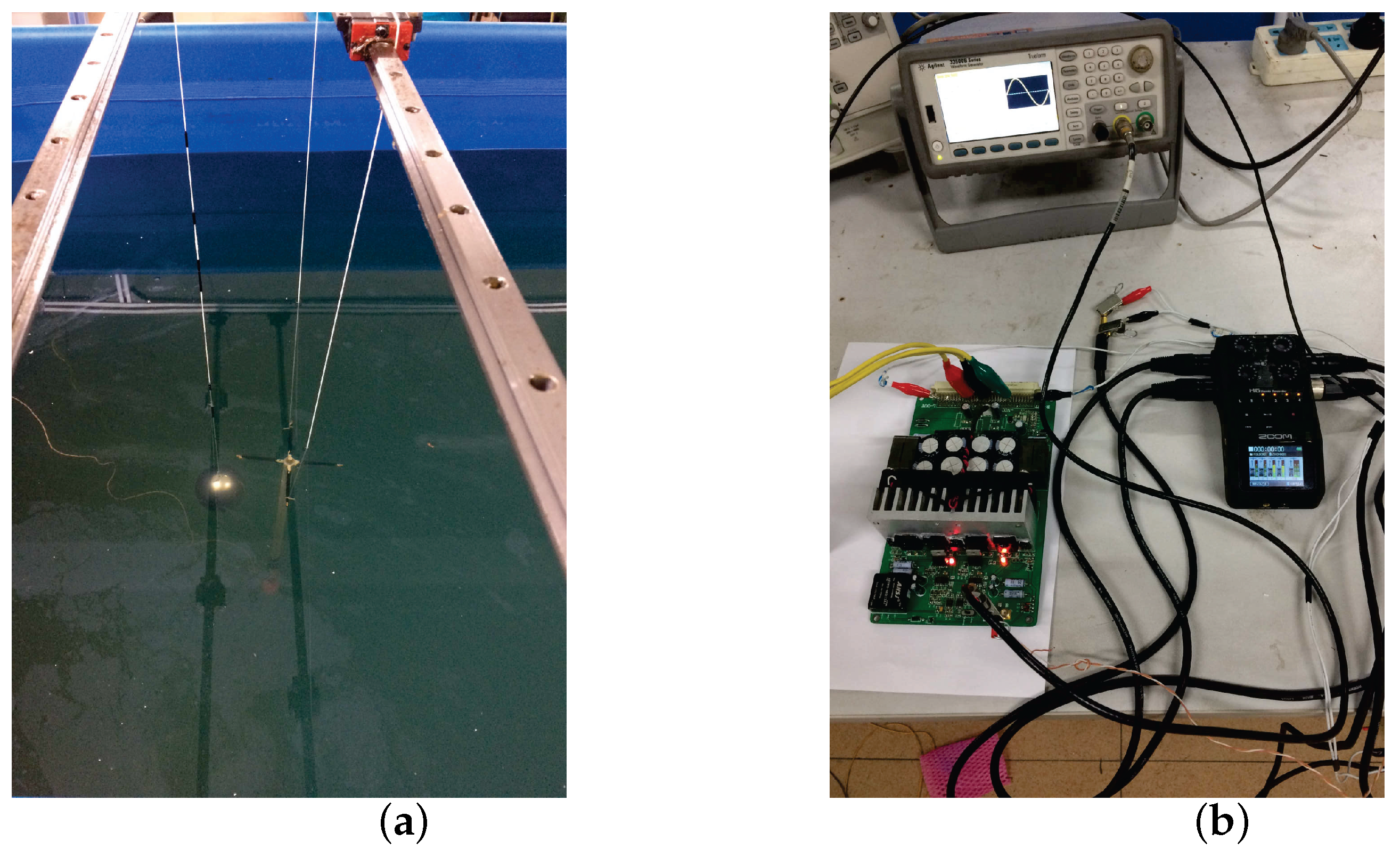
In order to further verify the effectiveness of the proposed locating method in reality, a set of physical experiments is developed in our laboratory environment. We create a UCA system with 5 electrodes and an electric dipole source. The image of the UCA system and the detailed sizes are shown in
Figure 13. A cylindrical plastic pipe is used as the frame of the UCA system, with a diameter of 20 mm. Two metal sheets cover the end of the cylindrical plastic pipe to act as the electrodes of the dipole source. Four plastic cylinders with diameters of 5 mm and lengths of 100 mm are fixed at the other end of the frame. The four plastic cylinders are set at the same plane, which is perpendicular to the frame. Four metal sheets cover the end of the plastic cylinders as the receiving electrodes. The fifth electrode or the reference electrode is situated at the top end of the frame, which is
mm from the plane of the four receiving electrodes. In
Figure 14, the UCA system is vertically set at the center of the water tank, the electric dipole source of which is powered by a high power amplifier. The 5 electrodes compose the four-channel receiver, which are connected to a voltage measurement device product, the ZOOM H6 Handy Recorder. The measured data in the ZOOM H6 Handy Recorder will be imported into the MATLAB calculator. Then, the calculator outputs the estimated result of the target. The depth of the water in the tank is
m, and the conductivity of the water is set to be 4 S/m, which is close to the conductivity of sea water. A spherical target with a diameter of 100 mm is mounted on a horizontal movable gantry workbench with a size of 3 m by
m, which allows us to move the target along the pre-programmed trail with high geometric resolution.
In this experiment, the frequency of the electric dipole source is 8 kHz, and the impedance of the electric dipole source is
. The output voltage of the power stage is
Vrms, yielding the output power of
W and dipole moment of
A·m. The positions of the electrodes in the UCA system are known and fixed, which are listed in
Table 1. During the measurement, we first set the conductor target at the point
, where
. As the voltage of each channel is weak in seawater, we use the ZOOM H6 Handy Recorder as the analog to digital converter (ADC) device, which has configurable gain from
–
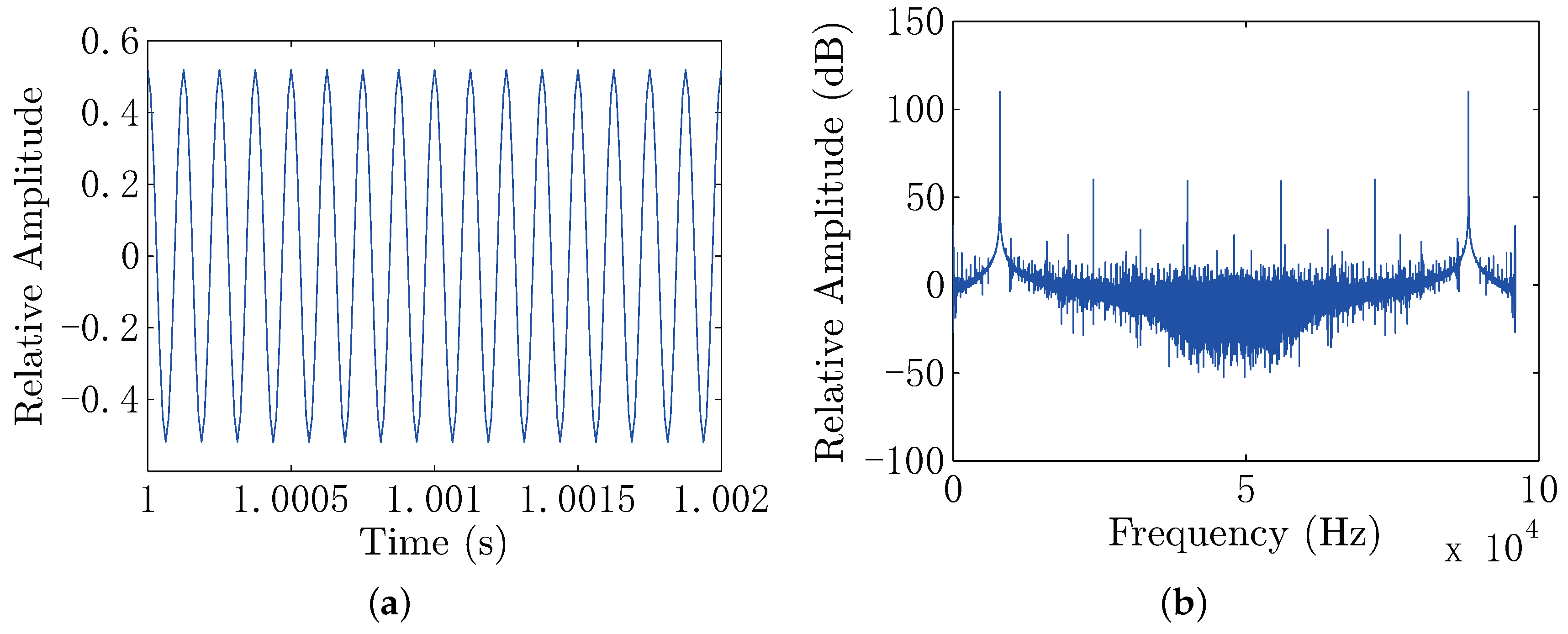
dB with a 96-kHz sample rate and 24-bit precision. We also do the same process for the insulator target. In this experiment, the measured voltage range of each channel is within 0.1∼15.6 mV. The measured signal contains noise shown in
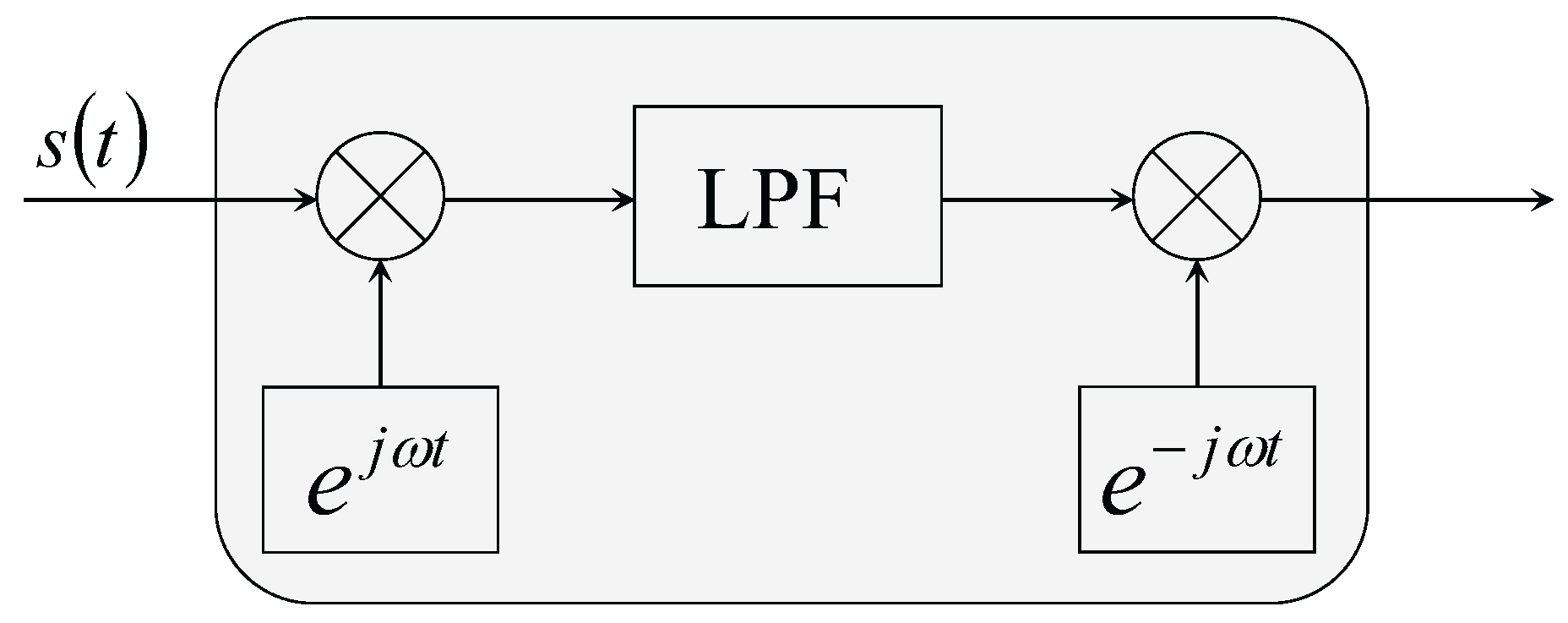
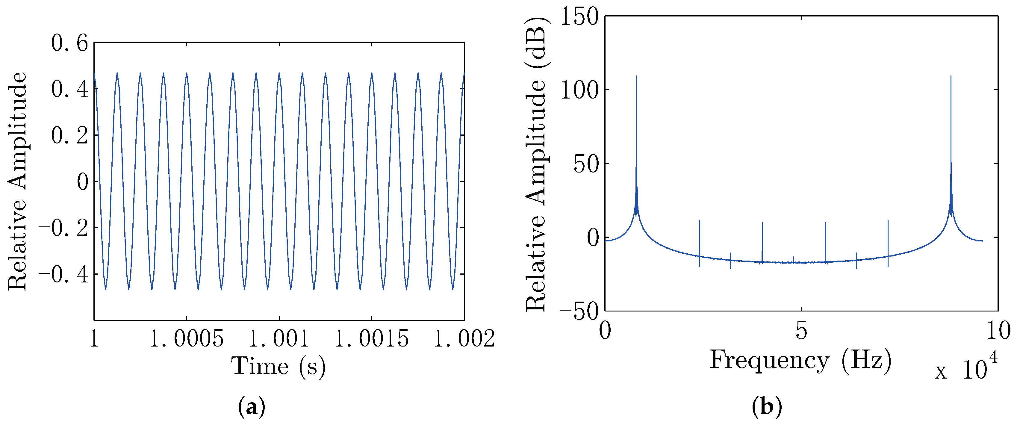
Figure 15, where the noise in the sea water is low, because of the high conductivity of the sea water, significantly shielding the electric noise and interference. In order to further filter the noise and interference, the digital filter is used in the background. The parameters of the digital filter of each channel are the same, which will not introduce additional gain distortion compared with the hardware filter on the front end. In this electro-locator system, the canonical high Q bandpass filter is used. We first shift the signal to the baseband. Then, we filter the baseband signal with a narrow band low pass filter, for which the coefficients are designed by the use of MATLAB FDATOOL. After that, the signal is shifted to the original frequency point. The canonical high Q bandpass filter is shown in
Figure 16, with the bandpass of 400 Hz. The filtered data are shown in
Figure 17, where the noise and interference are reduced after the digital filter.
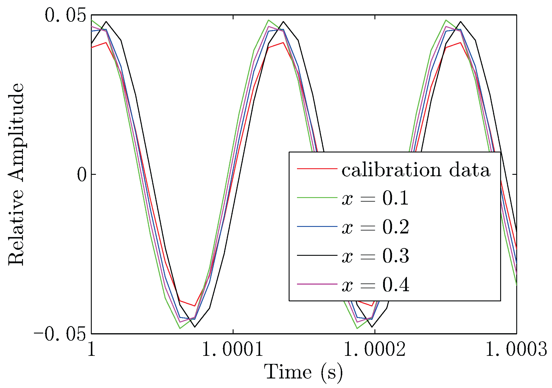
In the practical situation, there will be position error when building the UCA system. To overcome this drawback, we add calibration during the locating process. The calibration data are obtained without the target in the sea water tank. Then, we measure the voltages when the target is situated in the tank shown in
Figure 18. It can be seen from
Figure 18 that the voltages vary when the target is placed at different positions in the tank. During the locating process, the input data are the difference between the measured data and the calibration data. Here, we give an example of the location process according to one part of the raw data, and the electro-locator will finally output the target position result.
Step 2: Calculate the input data, the matrix , yielding the covariance matrix , where is a factor lager than zero;
Step 3: Get the eigenvector and eigenvalue by eigenvalue-decomposition. Here, we have , , where is a factor lager than zero. Thus, the signal subspace is , and the noise subspace projection matrix is ;
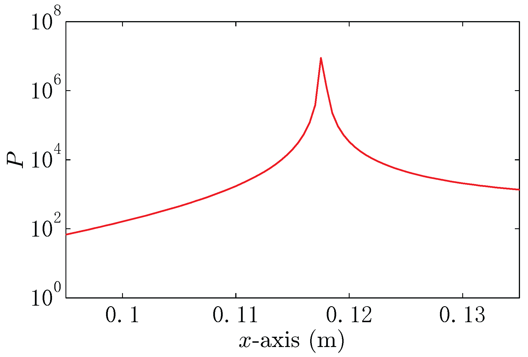
Step 4: Scan the observation area where the target exists with a series locating hypothesis and calculate the space spectrum. Here, we give the space spectrum near the target, which is shown in
Figure 19;
Step 5: From
Figure 19, we can see that the position corresponding to the peak of the spectrum is
, which is close to the true position
.
The estimated positions and their actual positions are also given in
Table 5, and we can find that the maximum location error is
m for the conductor target and
m for the insulator target. However, the location errors of the other points are less than
m. The estimation errors may be due to the following reasons. Firstly, the electric dipole source in the UCA system is not an ideal dipole, which has physical dimension errors in practice. Secondly, the frame of the UCA system can affect the distribution of the electric field. Thirdly, the electrodes’ position deviations are introduced to build the UCA system, resulting in locating errors. Finally, the actual positions of the target and the UCA system may be slightly moved during measurement because of the water wave. Although some experimental results slightly offset the center position, the localization accuracy is still good. These results prove that the proposed localization scheme can be applied to underwater target locating.


