Abstract
Land use changes remain one of the leading global change drivers leading to biodiversity loss in terrestrial and aquatic systems. Restoration aims to counteract the development of “natural” (i.e., forested, grassland, or wetland) spaces that alter and fragment the landscape and reduce local biodiversity through direct impacts to the water column and indirect impacts which inhibit adult dispersal of aquatic insects. This case study seeks to determine if a large-scale restoration of a former cranberry bog in Plymouth, MA has resulted in near-term measurable changes to the composition, structure, and function of local-scale in-stream habitat diversity. A three-year observational field study beginning one year prior to reconstruction was conducted at the restored cranberry bog and at two control treatment sites: an active cranberry bog reference and a least impacted reference (i.e., has never been used for modern agriculture). Seasonal inventories of in-stream habitat features including depth, substrate, macrohabitat, and in-stream cover were taken from 2015 to 2017. We found that 2 years post-restoration, there was no significant evidence of compositional or functional change, while there was a significant increase in structural diversity. There is reason to suspect the system is still in flux and longer-term monitoring may detect future habitat heterogeneity alterations.
1. Introduction
Human modification of stream systems and their surrounding landscapes has led to significant aquatic biodiversity declines and increased risk of future declines [1]. Land use change and habitat loss are recognized as leading global drivers of biodiversity change, and the most significant ones for the future of streams and rivers [2]. Indeed, land use changes have been implicated in degradation of stream biological conditions at both the local and catchment scale [3,4]. To combat this, restoration or remediation of impaired landscapes has been occurring with increasing frequency [5,6], often with varying goals including both social and ecological [7]. Freshwater systems are particularly amenable to guided and process-based restorative actions, allowing for greater potential of directed outcomes [8]. Due to the expense of these projects, effort often is undertaken at the local, or “reach”, scale, and as a result the ecological outcome is often unclear, due to limited investment in monitoring and the confounding factors of larger watershed impact [9,10].
Ecological restoration aimed at biodiversity recovery primarily employs methods intended to create habitat heterogeneity [11]. However, restoration outcomes are largely evaluated with respect to biotic changes, particularly in the case of target species [6]. This is especially true in the near term, as examinations of the success of habitat rehabilitation are performed across larger temporal and spatial scales [12]. Disparate methods of quantifying stream disturbance recoveries also make larger scale meta-analysis difficult. Often, studies only incorporate measures directly related to their goals or the major component of a system stressor [10].
Using the biodiversity framework set forth by Noss [13], measures of local-scale habitat can be broken down into one of three attributes: compositional, functional, and structural. These three components of habitat provide animal assemblages with the template for survival within an ecosystem: patch presence, functional requirements, and patch distribution, respectively. It is critical to consider the effect of scale on habitat features relevant to the assemblage being investigated [14]. At the reach (local) scale, composition can be measured through the abundance and diversity of in-stream cover types and river bottom substrates. River sinuosity within a system or a reach acts as a structural assessment of spatial variation, as sinuosity has been shown to impact habitat patch size separately from width or discharge/velocity [15]. Discrete units of sub-reach-scale habitat, known as macrohabitats, contain their own subset of interlinked functional processes, including decomposition within pools and oxygenation at riffle beds [16,17]. These reach-scale habitat measures can be combined into a holistic assessment of in-stream habitat heterogeneity, but also may be investigated independently as areas of potential habitat improvement in one component (sensu Noss, 1990) of biodiversity. While all three components address different aspects of habitat benefit to community assemblages, a combined metric of habitats’ composition, structure, and function can be calculated to assess the relative heterogeneity of the system.
The goal of this study was to determine if restoration resulted in any quantifiable near-term changes to the habitat at the local (i.e., reach) scale, and how those changes compared to control sites of high and low habitat diversity. To investigate early changes from restoration, we performed a three-year field study of a headwater stream conversion from flow-through cranberry bog use, following a before–after–control–impact design. We conducted reach-scale habitat evaluations seasonally beginning 1 year prior to the active phase of stream restoration, both at the restoration site and control sites of high and low habitat heterogeneity. We evaluated change through time via effect size analysis and change relative to controls via ANOVA. Local-scale habitat measures were expected to demonstrate separation of all three treatments following principal component analysis, as well as a separation of post-restoration CBR from pre-restoration clustering. Measures of compositional and structural heterogeneity were expected to increase following restoration, while functional change was not expected to occur within the timespan of the study. Finally, station sinuosity at CBR was expected to increase as a result of the rechannelization process.
2. Materials and Methods
2.1. Study Area
This study was conducted at three (3) treatments, representing restoration (cranberry bog restoration, Tidmarsh Farms, CBR), a least impacted reference stream (Mashpee River, LIR), and an unrestored agricultural system (active cranberry bog, ACB) in three separate low-order (1st–3rd) streams fed by primarily groundwater and drainage-fed ponds in the Atlantic Coastal Pine Barrens Ecoregion of Massachusetts (Figure 1). Each treatment consisted of three (3) replicate stations defined as a 100 m length segment where data was collected. Each station was separated by at least 100 m, to a maximum of 500 m, in river channel length and surveyed during base flow once per season (defined as astronomical spring, summer, and fall). Additional catchment and site-specific details of the three treatments are provided in the supplemental material (Supplemental Table S1).
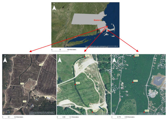
Figure 1.
Experimental treatment study locations and their relative locations in Southeastern Massachusetts. From left to right: Tidmarsh Farms (CBR, pre-restoration imagery), an active flow-through cranberry bog (ACB), and the Mashpee River flowing through the Trustees of Reservations conservation land (LIR) Maps produced with ArcGIS 10.4 [19].
2.2. Restoration Description
CBR underwent active ecological restoration in winter 2015/2016 after 5 years of passive restoration, which included the cessation of harvest management, as well as the removal of water control mechanisms. These active restoration activities took place over 0.78 km2 of property, ~10% of the entire catchment as measured from property outflow. The goals of the restoration included the re-establishment of groundwater connectivity, the creation of habitat complexity, and the overall intention to improve aquatic, microbial, and terrestrial biodiversity. Active restoration involved the rechannelization of 5.6 km of stream across the landscape and removal of dams, culverts, and other water control mechanisms. Additional landscape manipulations included the creation of microtopography, introduction of large woody debris to the channel, tens of thousands of individual native tree and shrub plantings, and the creation of water-retaining depressions and flow-through ponds to elevate the water table [18]. The cost of the restoration from federal, state, and private sources totaled more than USD 3 million. All stations surveyed for this project were within the bounds of the restoration area, along the original stream channel (2015) and along the newly cut channel (2016 and 2017).
2.3. Local-Scale Habitat Analysis
We conducted habitat assessments to quantify between treatment differences at the local scale, using the Basin Area Stream Survey (BASS) habitat inventory seasonally at all 100 m stations over the 3 year study [20]. Briefly, BASS delineates macrohabitats (i.e., riffles, runs, and pools) and performs cross-stream transects of each available macrohabitat at its midpoint. BASS measures include the number and length of each macrohabitat and the width, depth, and substrate profile of each macrohabitat, as well as estimation of in-stream habitat features, including bare substrate, rooted aquatic plants, adherent/clinging algae, large or small woody debris, or undercut embankments. Values were recorded in the field and analyzed by principal component analysis using the vegan package in R [21,22] to determine variability between treatments and across time.
The raw BASS data also was used to generate four composite measures of in-stream habitat diversity. Diversity of in-stream cover (Hcov) was calculated as the Shannon-Weiner index of the surface percentage of in-stream cover features. Diversity of substrate (Hsub) was similarly calculated as the Shannon-Weiner index of the percent cover for each substrate class. Standard deviation of depth (SDdep) was taken across the transect, and number of macrohabitats (Nhab) was calculated per 100 m station. Each parameter of the metric represents an attribute of biodiversity (e.g., composition, structure, or function), allowing for determination of not only overall habitat shifts, but also the local change drivers that may be acting within a system. For analysis, all transect-based parameters were averaged across the 100 m station, weighted by the length of their macrohabitat within the reach.
ArcGIS [19] was used to calculate stream sinuosity from aerial photography before and after the restoration event at all stations. Sinuosity was calculated as the river distance divided by the straight-line distance, as determined by station GPS coordinates, then assessed using one-way ANOVA, with treatment (ACB, LIR, and CBR before and after restoration) acting as predictors (n = 3 per treatment).
2.4. Statistical Analysis
The individual habitat diversity parameters were analyzed for effect size of change relative to control treatment following effect size for a BACI design:
where represents the mean parameter value in the “after” period while represents the mean value for the parameter “before” (e.g., in 2015, the initial year of study) for both , impact treatment, and , control treatment [23]. Confidence intervals (95%) were generated based on these effect sizes and pooled variance:
where and represent the variances and sample size for each set of treatment/period combinations [23]. This calculation was performed for both 2016 and 2017 as separate “after” periods, as we make no assumption of a stepwise change immediately following restoration combination, comparable to a before–during–after–control–impact study [24]. Additionally, due to the differences between control sites, separate analyses were run treating ACB or LIR as the control site. These analyses were completed for all four parameters. Effect sizes were determined to be statistically significant if the confidence interval did not overlap zero.
Additionally, within-year comparisons between CBR and the two control sites were conducted for each parameter using Welch’s corrected t-tests, due to nonhomogenous variation between treatments. For each parameter, CBR was compared to LIR and ACB in each of the 3 years of study. To account for repeated comparisons, the significance level (α) was lowered following a Bonferroni correction.
3. Results
3.1. Habitat Characterization PCA
Principal component analysis of local-scale habitat variables demonstrated habitat separation of LIR from CBR and ACB, while ACB clusters were within the variation observed at CBR (Figure 2). LIR transects were significantly more positive than either CBR or ACB along principal component (PC) 1 as determined by ANOVA (spring: F = 213.6, df = 2, p < 0.001, summer: F = 254.4, df = 2, p < 0.001, fall: F = 142.1, df = 2, p < 0.001) and subsequent post-hoc Tukey’s HSD (p < 0.001) (Supplemental Figure S1). PC1 was correlated negatively with habitat length and percent clinging vegetation, while PC2 was moderately correlated with habitat length, wetted width, and clinging and rooted vegetation (Table 1). Additionally, ACB habitat clusters were within the variation shown for CBR habitat, with the exception of significant differences along PC2 in the spring (Supplemental Figure S1).
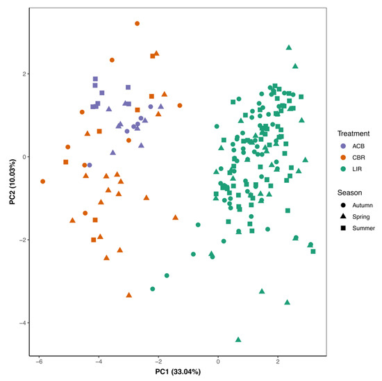
Figure 2.
PCA of local habitat transect data (BASS) from 2015–2017, coded by treatment (color) and season (shape) [21,22].

Table 1.
Loading values for each original variable on the first two principal components after PCA analysis of the local-scale habitat data from all three treatments across all three years.
When examined by year, CBR also showed change following restoration (Figure 3A). CBR showed significant decline along PC1 (F = 11.2, df = 2, p < 0.001, Figure 3B) and PC2 (F = 26.95, df = 2, p < 0.001, Figure 3C) from 2015 to both 2016 and 2017, as determined by ANOVA and subsequent Tukey’s HSD (p < 0.01). These findings are robust to separate analysis by season (Supplemental Table S2).
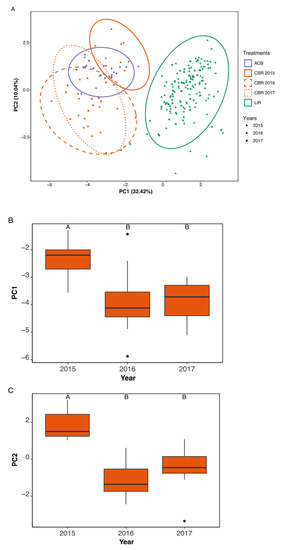
Figure 3.
PCA of local habitat transect data (BASS) from 2015–2017, coded by treatment (color) and year (shape), with 95% confidence interval ellipses for group centroid based on standard deviation (outlining ellipses) (A). ANOVAs of CBR data along PC1 (B) and PC2 (C), with significantly different values (α = 0.05) within each graph, as determined by Tukey’s HSD, marked by different letters; shared letters represent nonsignificant differences [21,22].
3.2. Habitat Heterogeneity
No significant seasonal differences were demonstrated in any of the four habitat heterogeneity parameters, and thus they were averaged by year to avoid issues with pseudoreplication (Supplemental Table S3). Only standard deviation of depth (SDdep) in 2017 demonstrated an effect size confidence interval that did not overlap zero (Supplemental Table S4). When comparing CBR to the reference conditions, changes in both substrate diversity (Hsub) and standard deviation of depth (SDdep) were observed (Supplemental Table S5).
In-stream cover diversity (Hcov) increased following restoration and continued to increase over the course of the study in 2016 and in 2017, but was not statistically significant (Figure 4A). Pairwise Welch’s corrected t-tests within year showed no significant differences between CBR and the other two treatments in any year (Figure 4B).
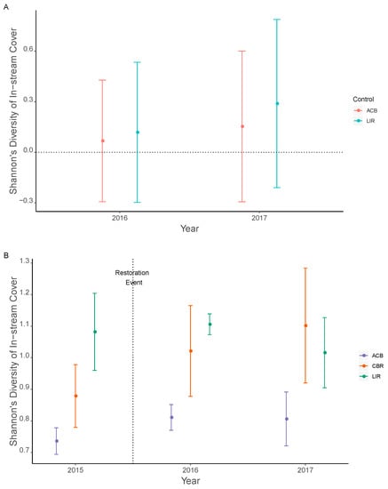
Figure 4.
Shannon’s diversity of in-stream cover (Hcov) as given by BACI effect size (A) and actual values with standard error (B). No significant differences are observed in effect size, with confidence interval ranges overlapping zero (A) while pairwise Welch’s t-tests were not significant (α = 0.008) between CBR and other treatments within each year (B). ACB = active cranberry bog, CBR = cranberry bog restoration, LIR = least impacted reference. All statistical comparisons are listed in Supplemental Tables S4A and S5B.
Substrate compositional diversity (Hsub) fell immediately following restoration in 2016, resulting in a statistically significant effect size change relative to LIR, but not ACB (dLIR = −0.387, CI: (−0.750, −0.024); dACB = −0.240, CI: (−0.533, 0.053)). However, in 2017 the substrate composition increased and was no longer significantly different relative to either control (Figure 5A). CBR was not significantly different from either other treatment in 2015 or 2017 but was significantly different than LIR in 2016 (Welch’s t = −5.295, ν = 3.874, p = 0.007) (Figure 5B).
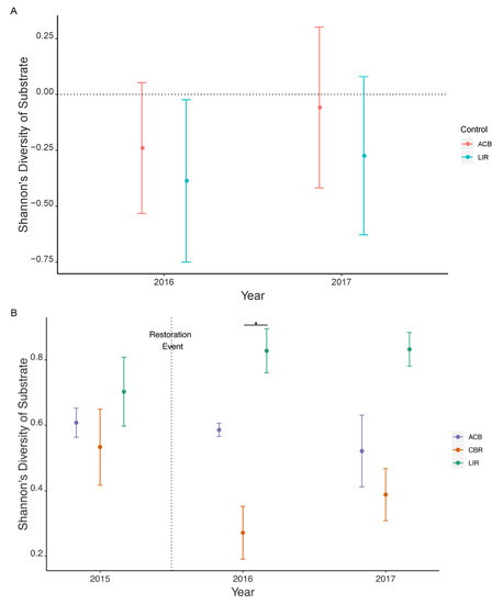
Figure 5.
Shannon’s diversity of substrate (Hsub) as given by BACI effect size (A) and actual values with standard error (B). Significant differences are noted by confidence interval range not overlapping zero (A) while pairwise Welch’s t-tests with significant differences (α = 0.008) between CBR and other treatments within each year are marked with (*) (B). ACB = active cranberry bog, CBR = cranberry bog restoration, LIR = least impacted reference. All statistical comparisons are listed in Supplemental Tables S4A and S5B.
Depth standard deviation (SDdep) significantly increased following restoration in 2016 (dLIR = 0.174 CI: (0.064, 0.285); dACB = 0.192, CI: (0.065, 0.319)), and, in 2017, remained significantly different relative to ACB control but not LIR (dLIR = 0.084, CI: (–0.001, 0.169); dACB = 0.152, CI: (0.097, 0.206)) (Figure 6A). Pairwise t-tests show no significant differences between CBR and LIR or ACB for any years (Figure 6B).
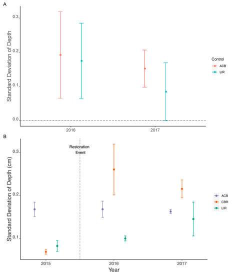
Figure 6.
Standard deviation of depth (SDdep) as given by BACI effect size (A) and actual values with standard error (B). Significant differences are noted by confidence interval range not overlapping zero (A) while all pairwise Welch’s t-tests are non-significant (α = 0.008) between CBR and other treatments within each year (B). ACB = active cranberry bog, CBR = cranberry bog restoration, LIR = least impacted reference. All statistical comparisons are listed in Supplemental Tables S4A and S5B.
Finally, the number of macrohabitats (Nhab) per 100 m at CBR increased in the first year post-restoration, followed by a slight decline in 2017, but neither were significant (Figure 7A). Pairwise t-tests demonstrated CBR as significantly different than LIR in 2015 (Welch’s t = −8.014, ν = 3.000, p = 0.004) and 2017 (Welch’s t = −7.475, ν = 3.329, p = 0.003) (Figure 7B).
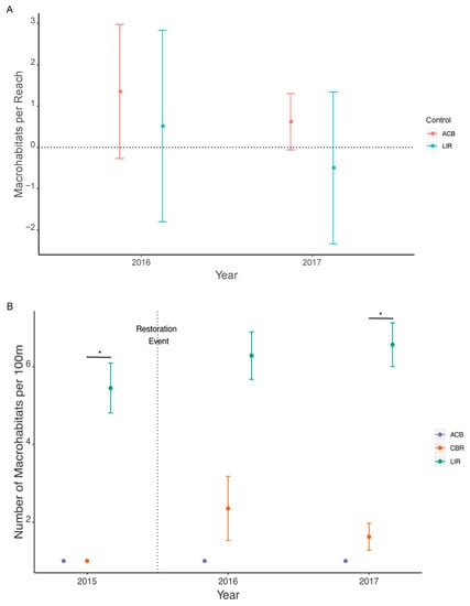
Figure 7.
Number of macrohabitats (Nhab) per 100 m as given by BACI effect size (A) and actual values with standard error (B). Significant differences are not observed for effect size, with confidence interval ranges not overlapping zero (A) while significant pairwise Welch’s t-tests (α = 0.008) between CBR and other treatments within each year are marked with (*) (B). ACB = active cranberry bog, CBR = cranberry bog restoration, LIR = least impacted reference. All statistical comparisons are listed in Supplemental Tables S4A and S5B.
3.3. Sinuosity
Channel morphology changes after restoration demonstrated an increase in sinuosity post-restoration; however, this difference is not statistically significant (F = 2.832, df = 3, p = 0.10) (Figure 8).
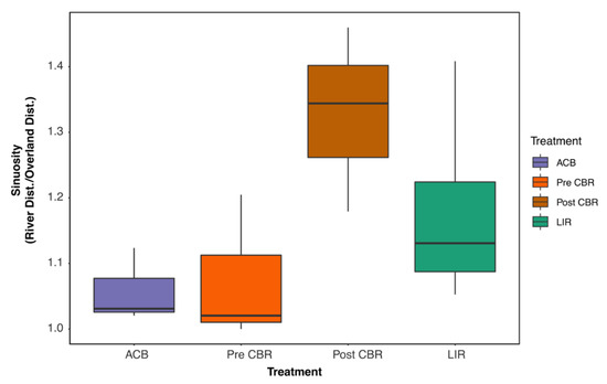
Figure 8.
Sinuosity at ACB (n = 3) and LIR (n = 4), as well as pre- (n = 3) and post-restoration (n = 3) at CBR. Treatments were not significantly different (α = 0.05). ACB and LIR sinuosity were unchanged in the same time period. ACB = active cranberry bog, CBR = cranberry bog restoration, LIR = least impacted reference.
4. Discussion
Overall, the results of our study lead to two main findings. First, CBR experienced a post-restoration shift in local-scale habitat based on a comprehensive habitat survey. However, after restoration, CBR values were more similar to ACB when examined by PCA. Second, when habitat heterogeneity metrics were investigated, local-scale changes did occur, but were limited to declines in substrate diversity and an increase in depth variation, both properties that are features of ACB rather than LIR.
The BASS habitat characterization PCA of transect data from all three treatments shows the expected separation between the unimpacted reference (LIR) and both the active (ACB) and restored cranberry bog (CBR). There was no clear separation between CBR and ACB within the PCA, contrary to our expectation that CBR would show unique habitat befitting its 5 years of passive restoration. PCA separation was driven largely by the relative length of the macrohabitats and the percentage of clinging vegetation. Both variables are tied to the anthropogenic impact cranberry farming imposes upon the system, through channelization and loss of riparian canopy cover, respectively [25,26]. This may demonstrate the legacy effects of agriculture [4,27] and the inability of low-gradient streams to adequately flush sediments [15] and reshape stream channels [28]. Much of the variability in CBR sites was found in the first year post-restoration, consistent with both a disturbance event and potential reorganization period [29]. Although there was no distinct separation of habitat, variation along PC2 does demonstrate some differences between ACB and CBR, especially for the first year of restoration. The associated variables of habitat length, channel width, and in-stream vegetation can be tied to the direct manipulation of the channel during the restoration.
When we examine the components of the habitat heterogeneity model for individual contributions to ecosystem level biodiversity, the results are complex. In-stream cover (Hcov) and substrate diversity (Hsub) can be considered aspects of compositional diversity due to the niches they create [30]. While neither in-stream cover nor substrate diversity show statistically significant shifts following restoration, both change in important ways. In-stream cover monotonically increases into the second year, allowing the possibility of sustained change in years following the study. Substrate diversity, on the other hand, declines in the first year and rebounds in the second, potentially operating as a pulse response to the rechannelization. This lack of change in compositional diversity runs contrary to our prediction of increased habitat compositional diversity as a result of the restorative actions, although significant changes may be masked by small sample size and high variability. Other studies that have found increases in composition post-restoration have either assessed later change following restoration [31,32] or monitored specific features following targeted interventions (e.g., width and flow changes following woody debris removal [33]). As a measure of structural diversity, standard deviation in depth (SDdep) was expected to be highest for the LIR treatment, as a diversity of depth may support a more diverse fish and invertebrate community [34]. However, the extreme variation in depth, from shallow along the bank to over a meter deep at maximum depth, makes the channels at CBR post-restoration and ACB sites exhibit a more diverse depth profile than LIR. Post-restoration, CBR depths became more varied, as the channel was flattened at the banks to promote flood plain interaction while deepening mid-channel to interface with the peat layer below the former farm surface [18]. Thus, CBR did exhibit structural increases in depth profile, but it remains to be seen whether this change will persist in long-term channel profiling. Finally, number of macrohabitats (Nhab) acted as a proxy for functional change, as macrohabitats have distinct microhabitats and alterations to water chemistry that may impact aquatic organisms [16]. Although macrohabitats increased at CBR following restoration, the increase was not statistically significant. Thus, our hypothesis that CBR would experience no functional change over the course of the study was upheld, although the increase observed in the first 2 years post-restoration may bear out as sustained and quantifiable functional change with continued monitoring.
As a final measure of structural change to the system, the post-restoration sinuosity increase was found to be not significantly different. Sinuosity has many functions within the stream channel, including decreasing sedimentation, slowing overall flow, and creating specialized pool habitats [15,35]. The lack of power due to limited sample size may explain why the increase was not significant.
The changes observed in the habitat suggest the restoration may have created initial changes in compositional, structural, and functional diversity beyond what we predicted as initial change only in the compositional attribute of habitat diversity. Given the lack of statistical power to determine significant shifts in many cases, whether the functional change persists after the reorganizational period remains to be seen. Many studies have suggested that functional change is necessary to accommodate community shifts, while compositional changes are more likely to occur first [11]. Ecosystem function also is highly tied to ecosystem resistance and resilience, potentially allowing community shifts to follow.
5. Conclusions
As restorations become more common tools to restore ecosystem functioning and promote biodiversity, the change in habitat at multiple scales cannot be ignored. Stream and terrestrial habitats operate at both the local scale and at the watershed scale, affecting key features such as population persistence or insect dispersal, respectively. At the reach scale, the characteristics of transect habitat suggest that restoration did not significantly alter the legacy of farming within the span of the three-year study. Individual components of reach-scale habitat demonstrate mixed effects, from no change in macrohabitat diversity or in-stream cover diversity, to transitory change in substrate diversity, with only depth variability maintaining its post-restoration change during the study period. Notably, however, we do see the highest changes in the first year of the restoration, suggesting expected disturbances from restoration activities. The high variability in habitat parameters at CBR in both years post-restoration also suggests that the system has not yet stabilized [36].
Although 3 years is a relatively short study and does not account for long-term changes to the riparian zone through reforestation, the activities undertaken as part of the active restoration were expected to present immediate and persistent changes to the reach-scale habitat through increases in sinuosity and the incorporation of woody debris. The goal of complex habitat creation requires targeted monitoring both in the near and longer terms [8]. The effect, however, appears to demonstrate a system still in flux regarding habitat parameters, with some evidence of pulse disturbance rather than maintained change.
Finally, this study is inherently limited in scope, due to the inclusion of only one restoration site, rather than several. As such, there is an increased risk of identifying patterns of change that are site specific, rather than broadly applicable. Further work validating these near-term changes in future cranberry bog restorations as well as longitudinal study of longer-term changes at cranberry bog restorations are merited. In order to limit site-specific effects, we recommend a space-for-time substitution study when more projects of this scope and methodology are completed.
Supplementary Materials
The following are available online at https://www.mdpi.com/article/10.3390/d13060235/s1, Table S1: Quantitative and qualitative descriptions of the three treatment sites, cranberry bog restoration (CBR), active cranberry bog (ACB), and least impacted reference (LIR). Catchment details were obtained through ArcGIS [19] using data provided by MassGIS [37]. Table S2: Cranberry bog restoration (CBR) change over time for principal components 1 and 2 of local scale habitat PCA (Figure 3). Post-hoc Tukey’s HSD was performed to determine pairwise significant differences. Significant values (p > 0.05) are bolded. Table S3: ANOVA result table of habitat heterogeneity parameters with season as predictor variable. Parameters are diversity of in-stream cover (Hcov), diversity of substrate (Hsub), number of macrohabitats (Nhab), and standard deviation of depth (SDdep), all of which have been averaged across the 100 m station by the weighted average of their habitat lengths. Table S4: Effect size (BACI) of change before and after restoration (2015 to 2016, or 2015 to 2017) relative to control (LIR or ACB) treatment. Each effect size is calculated as described in text, with 95% confidence intervals generated from pooled variance. Bolding represents effects with confidence intervals not overlapping 0. ACB = active cranberry bog, CBR = cranberry bog restoration, LIR = least impacted reference. Table S5: Within-year differences between CBR and control treatments. T values represent Welch’s two-tailed t-tests between CBR and listed treatment in the same year. Due to unequal variances, Welch’s t-tests calculate ν, a modified df. Bolding represents changes that are significantly different (α = 0.008, Bonferroni correction for six comparisons per year). ACB = active cranberry bog, CBR = cranberry bog restoration, LIR = least impacted reference. Figure S1: ANOVA results for Principal Components 1 and 2 from local scale habitat transect (BASS) data. Analysis was performed within seasons to avoid confounding variables from seasonal change. PC1 in spring (A), PC1 in spring (A), PC2 in spring (B), PC1 in summer (C), PC2 in summer (D), PC1 in fall (E), PC2 in fall (F). Significantly different values within each graph, as determined by Tukey’s HSD, are marked with different letters; shared letters represent nonsignificant differences.
Author Contributions
Conceptualization, S.T.M. and A.D.C.; methodology, S.T.M. and A.D.C.; analysis, S.T.M.; investigation, S.T.M.; field work, S.T.M. and T.F.D.; data curation, S.T.M. and T.F.D.; writing—original draft preparation, S.T.M. and A.D.C.; writing—review and editing, S.T.M. and A.D.C.; visualization, S.T.M.; supervision, A.D.C.; project administration, A.D.C.; funding acquisition, A.D.C. All authors have read and agreed to the published version of the manuscript.
Funding
Funding for this research was provided by Alan Christian through both the Biology Department and School for the Environment at the University of Massachusetts Boston (UMB), as well as the Distinguished Doctoral Fellowship (UMB) and UMB’s Coasts and Communities NSF IGERT Fellowship (NSF Award Number 1249946). Additional funds were secured through the crowdfunding site Experiment.com, as well as the UMB Biology Department’s Doctoral Dissertation Improvement Grant and Lipke Travel Grants.
Data Availability Statement
Data is held with S.T.M. and A.D.C. and available upon request.
Acknowledgments
Additional intellectual contributions and feedback were provided by Robert Stevenson, Thilina Surasinghe, Michael Shiaris, and Jarrett Byrnes. Field help was provided by the entire Freshwater Ecology Lab and many years of Coastal Research in Environmental Science (CREST) REU students and volunteer interns. We also thank Living Observatory and the Massachusetts Division of Ecological Restoration for site access, additional details on restoration activities, and coordination of sampling activities.
Conflicts of Interest
S.T.M. and A.D.C. currently serve as guest editors for Diversity’s Special Issue on Aquatic Restoration Ecology and Monitoring, for which this manuscript is under consideration.
References
- Janse, J.H.; Kuiper, J.J.; Weijters, M.J.; Westerbeek, E.P.; Jeuken, M.H.J.L.; Bakkenes, M.; Alkemade, R.; Mooij, W.M.; Verhoeven, J.T.A. GLOBIO-Aquatic, a Global Model of Human Impact on the Biodiversity of Inland Aquatic Ecosystems. Environ. Sci. Policy 2015, 48, 99–114. [Google Scholar] [CrossRef]
- Sala, O.E.; Chapin, F.S.; Armesto, J.J.; Berlow, E.; Bloomfield, J.; Dirzo, R.; Huber-Sanwald, E.; Huenneke, L.F.; Jackson, R.B.; Kinzig, A.; et al. Biodiversity—Global Biodiversity Scenarios for the Year 2100. Science 2000, 287, 1770–1774. [Google Scholar] [CrossRef]
- Bierschenk, A.M.; Mueller, M.; Pander, J.; Geist, J. Impact of Catchment Land Use on Fish Community Composition in the Headwater Areas of Elbe, Danube and Main. Sci. Total Environ. 2019, 652, 66–74. [Google Scholar] [CrossRef] [PubMed]
- Knott, J.; Mueller, M.; Pander, J.; Geist, J. Effectiveness of Catchment Erosion Protection Measures and Scale-Dependent Response of Stream Biota. Hydrobiologia 2019, 830, 77–92. [Google Scholar] [CrossRef]
- BenDor, T.; Lester, T.W.; Livengood, A.; Davis, A.; Yonavjak, L. Estimating the Size and Impact of the Ecological Restoration Economy. PLoS ONE 2015, 10, e0128339. [Google Scholar] [CrossRef] [PubMed]
- Palmer, M.A.; Menninger, H.L.; Bernhardt, E. River Restoration, Habitat Heterogeneity and Biodiversity: A Failure of Theory or Practice? Freshw. Biol. 2010, 55, 205–222. [Google Scholar] [CrossRef]
- Smith, R.F.; Hawley, R.J.; Neale, M.W.; Vietz, G.J.; Diaz-Pascacio, E.; Herrmann, J.; Lovell, A.C.; Prescott, C.; Rios-Touma, B.; Smith, B.; et al. Urban Stream Renovation: Incorporating Societal Objectives to Achieve Ecological Improvements. Freshw. Sci. 2016, 35, 364–379. [Google Scholar] [CrossRef]
- Geist, J.; Hawkins, S.J. Habitat Recovery and Restoration in Aquatic Ecosystems: Current Progress and Future Challenges. Aquat. Conserv. Mar. Freshw. Ecosyst. 2016, 26, 942–962. [Google Scholar] [CrossRef]
- Bernhardt, E.S.; Palmer, M.A. River Restoration: The Fuzzy Logic of Repairing Reaches to Reverse Catchment Scale Degradation. Ecol. Appl. 2011, 21, 1926–1931. [Google Scholar] [CrossRef]
- Palmer, M.A.; Bernhardt, E.S.; Allan, J.D.; Lake, P.S.; Alexander, G.; Brooks, S.; Carr, J.; Clayton, S.; Dahm, C.N.; Follstad Shah, J.; et al. Standards for Ecologically Successful River Restoration. J. Appl. Ecol. 2005, 42, 208–217. [Google Scholar] [CrossRef]
- Palmer, M.A.; Hondula, K.L.; Koch, B.J. Ecological Restoration of Streams and Rivers: Shifting Strategies and Shifting Goals. Annu. Rev. Ecol. Evol. Syst. 2014, 45, 247–269. [Google Scholar] [CrossRef]
- Jähnig, S.C.; Brabec, K.; Buffagni, A.; Erba, S.; Lorenz, A.W.; Ofenböck, T.; Verdonschot, P.F.M.; Hering, D. A Comparative Analysis of Restoration Measures and Their Effects on Hydromorphology and Benthic Invertebrates in 26 Central and Southern European Rivers. J. Appl. Ecol. 2010, 47, 671–680. [Google Scholar] [CrossRef]
- Noss, R.F. Indicators for Monitoring Biodiversity: A Hierarchical Approach. Conserv. Biol. 1990, 4, 355–364. [Google Scholar] [CrossRef]
- Death, R.G.; Joy, M.K. Invertebrate Community Structure in Streams of the Manawatu–Wanganui Region, New Zealand: The Roles of Catchment versus Reach Scale Influences. Freshw. Biol. 2004, 49, 982–997. [Google Scholar] [CrossRef]
- Auerswald, K.; Geist, J. Extent and Causes of Siltation in a Headwater Stream Bed: Catchment Soil Erosion Is Less Important than Internal Stream Processes. Land Degrad. Dev. 2018, 29, 737–748. [Google Scholar] [CrossRef]
- Frissell, C.A.; Liss, W.J.; Warren, C.E.; Hurley, M.D. A Hierarchical Framework for Stream Habitat Classification: Viewing Streams in a Watershed Context. Environ. Manag. 1986, 10, 199–214. [Google Scholar] [CrossRef]
- Poff, N.L. Landscape Filters and Species Traits: Towards Mechanistic Understanding and Prediction in Stream Ecology. J. N. Am. Benthol. Soc. 1997, 16, 391–409. [Google Scholar] [CrossRef]
- Living Observatory. Learning from the Restoration of Wetlands on Cranberry Farmland: Preliminary Benefits Assessment; Living Observatory, Inc.: Boston, MA, USA, 2020; p. 21. Available online: http://www.livingobservatory.org/learning-report (accessed on 27 May 2021).
- ESRI. ArcGIS Desktop Release 10.4.1; Environmental Systems Research Institute: Redlands, CA, USA, 2016. [Google Scholar]
- McCain, M.; Fuller, D.; Decker, L.; Overton, K. Stream Habitat Classification and Inventory Procedures for Northern California; U.S. Dept. of Agriculture, Forest Service, Pacific Southwest Region: San Francisco, CA, USA, 1990; pp. 1–16. [Google Scholar]
- Oksanen, J.; Blanchet, F.G.; Friendly, M.; Kindt, R.; Legendre, P.; McGlinn, D.; Minchin, P.R.; O’Hara, R.B.; Simpson, G.L.; Solymos, P.; et al. Vegan: Community Ecology Package, R package version 2.5-3; 2018. Available online: https://CRAN.R-project.org/package=vegan (accessed on 27 May 2021).
- R Core Team. A Language and Environment for Statistical Computing; R Foundation for Statistical Computing: Vienna, Austria, 2018. [Google Scholar]
- Christie, A.P.; Amano, T.; Martin, P.A.; Shackelford, G.E.; Simmons, B.I.; Sutherland, W.J. Simple Study Designs in Ecology Produce Inaccurate Estimates of Biodiversity Responses. J. Appl. Ecol. 2019, 56, 2742–2754. [Google Scholar] [CrossRef]
- Roedenbeck, I.; Fahrig, L.; Findlay, C.S.; Houlahan, J.; Jaeger, J.; Klar, N.; Kramer-Schadt, S.; van der Grift, E. The Rauischholzhausen Agenda for Road Ecology. Ecol. Soc. 2007, 12, 11. [Google Scholar] [CrossRef]
- Kristensen, E.A.; Thodsen, H.; Dehli, B.; Kolbe, P.E.Q.; Glismand, L.; Kronvang, B. Comparison of Active and Passive Stream Restoration: Effects on the Physical Habitats. Geogr. Tidsskr. Dan. J. Geogr. 2013, 113, 109–120. [Google Scholar] [CrossRef]
- Sudduth, E.B.; Hassett, B.A.; Cada, P.; Bernhardt, E.S. Testing the Field of Dreams Hypothesis: Functional Responses to Urbanization and Restoration in Stream Ecosystems. Ecol. Appl. 2011, 21, 1972–1988. [Google Scholar] [CrossRef]
- Maloney, K.O.; Weller, D.E. Anthropogenic Disturbance and Streams: Land Use and Land-use Change Affect Stream Ecosystems via Multiple Pathways. Freshw. Biol. 2011, 56, 611–626. [Google Scholar] [CrossRef]
- Waite, I.R. Agricultural Disturbance Response Models for Invertebrate and Algal Metrics from Streams at Two Spatial Scales within the U.S. Hydrobiologia 2014, 726, 285–303. [Google Scholar] [CrossRef]
- Stanley, E.H.; Powers, S.M.; Lottig, N.R. The Evolving Legacy of Disturbance in Stream Ecology: Concepts, Contributions, and Coming Challenges. J. N. Am. Benthol. Soc. 2010, 29, 67–83. [Google Scholar] [CrossRef]
- Bond, N.R.; Lake, P.S. Ecological Restoration and Large-Scale Ecological Disturbance: The Effects of Drought on the Response by Fish to a Habitat Restoration Experiment. Restor. Ecol. 2005, 13, 39–48. [Google Scholar] [CrossRef]
- Friberg, N.; Kronvang, B.; Ole Hansen, H.; Svendsen, L.M. Long-Term, Habitat-Specific Response of a Macroinvertebrate Community to River Restoration. Aquat. Conserv. Mar. Freshw. Ecosyst. 1998, 8, 87–99. [Google Scholar] [CrossRef]
- Kupilas, B.; Hering, D.; Lorenz, A.W.; Knuth, C.; Gücker, B. Hydromorphological Restoration Stimulates River Ecosystem Metabolism. Biogeosciences 2017, 14, 1989–2002. [Google Scholar] [CrossRef]
- Dumke, J.D.; Hrabik, T.R.; Brady, V.J.; Gran, K.B.; Regal, R.R.; Seider, M.J. Channel Morphology Response to Selective Wood Removals in a Sand-Laden Wisconsin Trout Stream. N. Am. J. Fish. Manag. 2010, 30, 776–790. [Google Scholar] [CrossRef]
- Lake, P.S. Ecological Effects of Perturbation by Drought in Flowing Waters. Freshw. Biol. 2003, 48, 1161–1172. [Google Scholar] [CrossRef]
- Brookes, A. Restoring the Sinuosity of Artificially Straightened Stream Channels. Environ. Geol. Water Sci. 1987, 10, 33–41. [Google Scholar] [CrossRef]
- Carpenter, S.R.; Brock, W.A. Rising Variance: A Leading Indicator of Ecological Transition. Ecol. Lett. 2006, 9, 311–318. [Google Scholar] [CrossRef] [PubMed]
- Bureau of Geographic Information. Bureau of Geographic Information (MassGIS); Commonwealth of Massachusetts, Executive Office of Technology and Security Services; 2016. Available online: https://www.mass.gov/info-details/massgis-data-layers (accessed on 27 May 2021).
Publisher’s Note: MDPI stays neutral with regard to jurisdictional claims in published maps and institutional affiliations. |
© 2021 by the authors. Licensee MDPI, Basel, Switzerland. This article is an open access article distributed under the terms and conditions of the Creative Commons Attribution (CC BY) license (https://creativecommons.org/licenses/by/4.0/).