
Three-Body Excitations in Fock-Space Coupled-Cluster: Fourth Order Perturbation Correction to Electron Affinity and Its Relation to Bondonic Formalism


Abstract
:1. Introduction
2. Theory Description: Basis Structure
3. Approximate Triplets: Perturbative Analysis
4. Bondonic Systematics of Electron Affinity Quantum Dynamics
5. Computational Details
6. Results and Discussion
7. Computational Cost
8. Conclusions
Supplementary Materials
Author Contributions
Institutional Review Board Statement
Informed Consent Statement
Data Availability Statement
Acknowledgments
Conflicts of Interest
References
- Crawford, T.D.; Stanton, J.F.; Allen, W.D.; Schaefer, H.F. Hartree-Fock Orbital Instability Envelopes in Highly Correlated Single-Reference Wavefunctions. J. Chem. Phys. 1997, 107, 10626–10632. [Google Scholar] [CrossRef]
- Bartlett, R.J.; Purvis, G.D., III. Many-body perturbation theory, coupled-pair many-electron theory, and the importance of quadruple excitations for the correlation problem. Int. J. Quantum Chem. 1978, 14, 561. [Google Scholar] [CrossRef]
- Lee, Y.S.; Kucharski, S.A.; Bartlett, R.J. A coupled cluster approach with triple excitations. J. Chem. Phys. 1984, 81, 5906. [Google Scholar] [CrossRef]
- Bartlett, R.J.; Sekino, H.; Purvis, G.D., III. Comparison of MBPT and coupled-cluster methods with full CI. Importance of triplet excitations and infinite summations. Chem. Phys. Lett. 1983, 98, 66–71. [Google Scholar] [CrossRef]
- Cizek, J. On the Correlation Problem in Atomic and Molecular Systems. Calculation of Wavefunction Components in Ursell-Type Expansion Using Quantum-Field Theoretical Methods. J. Chem. Phys. 1966, 45, 4256. [Google Scholar] [CrossRef]
- Sinanoglu, O. Many-Electron Theory of Atoms and Molecules. I. Shells, Electron Pairs vs Many-Electron Correlations. J. Chem. Phys. 1967, 36, 706–717. [Google Scholar] [CrossRef]
- Kucharski, S.A.; Lee, Y.S.; Purvis, G.D., III; Bartlett, R. Dipole polarizability of the fluoride ion with many-body methods. J. Phys. Rev. A 1984, 29, 1619. [Google Scholar] [CrossRef]
- King, B.T.; Michl, J. The Explosive “Inert” Anion CB11(CF3)12−. J. Am. Chem. Soc. 2000, 122, 10255–10256. [Google Scholar] [CrossRef]
- Asmis, K.R.; Taylor, T.R.; Neumark, D.M. Electronic structure of indium phosphide clusters: Anion photoelectron spectroscopy of InxPx− and Inx+1Px−(x = 1–13) clusters. Chem. Phys. Lett. 1999, 308, 347–354. [Google Scholar] [CrossRef]
- Greenblatt, B.J.; Zanni, M.T.; Neumark, D.M. Photodissociation of I2−(Ar)nClusters Studied with Anion Femtosecond Photoelectron Spectroscopy. Science 1997, 276, 1675–1678. [Google Scholar] [CrossRef]
- Cory, M.G.; Zerner, M.C. Calculation of the Electron Affinities of the Chromophores Involved in Photosynthesis. J. Am. Chem. Soc. 1996, 118, 4148. [Google Scholar] [CrossRef]
- Desfrancois, C.; Abdoul-Carime, H.; Carles, S.; Périquet, V.; Schermann, J.P.; Smith, D.M.A.; Adamowicz, L. Experimental and theoretical ab initio study of the influence of N-methylation on the dipole-bound electron affinities of thymine and uracil. J. Chem. Phys. 1999, 110, 11876. [Google Scholar] [CrossRef]
- Hehre, W.J.; Radom, L.; Schleyer, P.V.R.; Pople, J.A. Ab Initio Molecular Orbital Theory; Wiley: New York, NY, USA, 1986. [Google Scholar]
- Radom, L. Structures of simple anions from ab initio molecular orbital calculations. Aust. J. Chem. 1976, 29, 1635–1640. [Google Scholar] [CrossRef]
- Simons, J.; Jordan, K.D. Ab initio electronic structure of anions. Chem. Rev. 1987, 87, 535–555. [Google Scholar] [CrossRef]
- Bartlett, R.J. Coupled-cluster approach to molecular structure and spectra: A step toward predictive quantum chemistry. J. Phys. Chem. 1987, 93, 1697–1708. [Google Scholar] [CrossRef]
- Crawford, T.D.; Schaefer, H.F. An Introduction to Coupled Cluster Theory for Computational Chemistry. Rev. Comput. Chem. 1999, 14, 33–136. [Google Scholar]
- Urban, M.; Noga, J.; Cole, S.J.; Bartlett, R.J. Towards a full CCSDT model for electron correlation. J. Chem. Phys. 1985, 83, 4041–4046. [Google Scholar] [CrossRef] [Green Version]
- Cole, S.J.; Bartlett, R.J. Comparison of MBPT and coupled cluster methods with full CI. II. Polarized basis sets. J. Chem. Phys. 1987, 86, 873–881. [Google Scholar] [CrossRef]
- Noga, J.; Bartlett, R.J.; Urban, M. Towards a full CCSDT model for electron correlation. CCSDT-n models. Chem. Phys. Lett. 1987, 134, 126–132. [Google Scholar] [CrossRef]
- Noga, J.; Bartlett, R.J. The full CCSDT model for molecular electronic structure. J. Chem. Phys. 1987, 86, 7041–7050. [Google Scholar] [CrossRef]
- Coester, F.; Kummel, H. Short-range correlations in nuclear wave functions. Nucl. Phys. 1960, 17, 477. [Google Scholar] [CrossRef]
- Cizek, J. On the Use of the Cluster Expansion and the Technique of Diagrams in Calculations of Correlation Effects in Atoms and Molecules. Adv. Chem. Phys. 1969, 14, 35. [Google Scholar]
- Paldus, J.; Cizek, J.; Shavitt, I. Correlation Problems in Atomic and Molecular Systems. IV. Extended Coupled-Pair Many-Electron Theory and Its Application to the BH3Molecule. Phys. Rev. A 1972, 5, 50. [Google Scholar] [CrossRef]
- Bartlett, R.J. Many-body perturbation theory and Coupled-cluster theory for electron correlation in molecule. Ann. Rev. Phys. Chem. 1981, 32, 359–401. [Google Scholar] [CrossRef]
- Meissner, L. Fock-space coupled-cluster method in the intermediate Hamiltonian formulation: Model with singles and doubles. J. Chem. Phys. 1998, 108, 9227. [Google Scholar] [CrossRef]
- Bartlett, R.J.; Watts, J.D.; Kucharski, S.A.; Noga, J. Non-iterative fifth-order triple and quadruple excitation energy Corrections in correlated methods. Chem. Phys. Lett. 1990, 165, 513–522. [Google Scholar] [CrossRef]
- Watts, J.D.; Gauss, J.; Bartlett, R.J. Coupled-cluster methods with noniterative triple excitations for restricted open-shell Hartree-Fock and other general single determinant reference functions. Energies and analytical gradients. J. Chem. Phys. 1993, 98, 8718–8733. [Google Scholar] [CrossRef]
- Kucharski, S.A.; Bartlett, R.J. Noniterative energy corrections through fifth-order to the coupled cluster singles and doubles method. J. Chem. Phys. 1998, 108, 5243–5254. [Google Scholar] [CrossRef]
- Paldus, J.; Li, X. A Critical Assessment of Coupled Cluster Method in Quantum Chemistry. Adv. Chem. Phys. 1999, 110, 1–175. [Google Scholar]
- Purvis, G.D., III; Bartlett, R.J. A full coupled-cluster singles and doubles model: The inclusion of disconnected triples. J. Chem. Phys. 1982, 76, 1910. [Google Scholar] [CrossRef]
- Raghavachari, K. Historical perspective on: A fifth-order perturbation comparison of electron correlation theories. Chem. Phys. Lett. 1989, 157, 479–483. [Google Scholar] [CrossRef]
- Pal, S. Multireference coupled cluster response approach for the calculation of static properties. Phys. Rev. A 1989, 39, 39–42. [Google Scholar] [CrossRef]
- Mukhejee, D.; Moitra, R.K.; Mukhopadhyay, A. Correlation problem in open-shell atoms and molecules. Mol. Phys. 1975, 30, 1861. [Google Scholar] [CrossRef]
- Pal, S.; Prasad, M.D.; Mukhejee, D. Development of a size-consistent energy functional for open shell states. Theoret. Chim. Acta 1984, 66, 313–332. [Google Scholar] [CrossRef]
- Haque, A.; Kaldor, U. Open-shell coupled-cluster theory applied to atomic and molecular systems. Chem. Phys. Lett. 1985, 117, 347–351. [Google Scholar] [CrossRef]
- Mukherjee, D. The linked-cluster theorem in the open-shell coupled-cluster theory for incomplete model spaces. Chem. Phys. Lett. 1986, 125, 207–212. [Google Scholar] [CrossRef]
- Sinha, D.; Mukhopadhyay, D.; Mukherjee, D. A note on the direct calculation of excitation energies by quasi-degenerate MBPT and coupled-cluster theory. Chem. Phys. Lett. 1986, 129, 369–374. [Google Scholar] [CrossRef]
- Pal, S.; Rittby, M.; Bartlett, R.J.; Sinha, D.; Mukherjee, D. Multireference coupled-cluster methods using an incomplete model space: Application to ionization potentials and excitation energies of formaldehyde. Chem. Phys. Lett. 1987, 137, 273–278. [Google Scholar] [CrossRef]
- Pal, S. Fock space multi-reference coupled cluster method for energies and energy derivatives. Mol. Phys. 2010, 108, 3033–3042. [Google Scholar] [CrossRef]
- Pal, S.; Rittby, M.; Bartlett, R.J.; Sinha, D.; Mukherjee, D. Molecular applications of multireference coupled-cluster methods using an Incomplete model space. J. Chem. Phys. 1988, 88, 4357–4365. [Google Scholar] [CrossRef]
- Rittby, M.; Pal, S.; Bartlett, R.J. Multi reference coupled cluster method: Ionization potentials and excitation energies of ketene and Diazomethane. J. Chem. Phys. 1989, 90, 3214–3220. [Google Scholar] [CrossRef]
- Ben-shlomo, S.; Kaldor, U. The open-shell coupled-cluster method in general model space: Five states of LiH. J. Chem. Phys. 1988, 89, 956. [Google Scholar] [CrossRef]
- Koch, S.; Mukherjee, D. Atomic and molecular applications of open-shell cluster expansion techniques with incomplete model spaces. Chem. Phys. Lett. 1985, 145, 321–328. [Google Scholar] [CrossRef]
- Mukherjee, D.; Pal, S. Use of Cluster expansion methods in the open shell correlation problem. Adv. Quantum Chem. 1989, 20, 291–373. [Google Scholar]
- Basumallick, S.; Sajeev, Y.; Vaval, N.; Pal, S. Negative Ion Resonance States: The Fock-Space Coupled-Cluster Way. J. Phys. Chem. A 2020, 50, 10407–10421. [Google Scholar] [CrossRef]
- Ajitha, D.; Vaval, N.; Pal, S. Multi-reference coupled cluster based analytic response approach for evaluating molecular properties: Some pilot results. J. Chem. Phys. 1999, 110, 2316–2322. [Google Scholar] [CrossRef]
- Ajitha, D.; Pal, S. Z-vector formalism for the Fock space multi-reference coupled cluster method: Elimination of the response of the highest valence sector amplitudes. J. Chem. Phys. 1999, 111, 3832–3836. [Google Scholar] [CrossRef]
- Shamasundar, K.R.; Asokan, S.; Pal, S. A constrained variational approach for energy derivatives in Fock space multi-reference coupled-cluster theory. J. Chem. Phys. 2004, 120, 6381–6398. [Google Scholar] [CrossRef]
- Sajeev, Y.; Santra, R.; Pal, S. Analytically continued Fock space multireference coupled-cluster theory: Application to the 2 Πg shape resonance in e-N2 scattering. J. Chem. Phys. 2005, 122, 234320. [Google Scholar] [CrossRef]
- Sajeev, Y.; Santra, R.; Pal, S. Correlated complex independent particle potential for calculating electronic Resonances. J. Chem. Phys. 2005, 123, 204110. [Google Scholar] [CrossRef]
- Basumallick, S.; Bhattacharyya, S.; Jana, I.; Vaval, N.; Pal, S. Shape resonance of sulphur dioxide anion excited states using the CAP-CIP-FSMRCCSD method. Mol. Phys. 2020, 118, e1726521. [Google Scholar] [CrossRef]
- Musial, M.; Bartlett, R.J. Intermediate Hamiltonian Fock-space multireference coupled-cluster method with full triples for calculation of excitation energies. J. Chem. Phys. 2008, 129, 044101. [Google Scholar] [CrossRef]
- Musial, M.; Bartlett, R.J. Fock space multireference coupled cluster method with full inclusion of connected triples for excitation energies. J. Chem. Phys. 2004, 121, 1670–1675. [Google Scholar] [CrossRef] [PubMed]
- Pal, S.; Rittby, M.; Bartlett, R.J. Multi reference coupled cluster methods for ionization potentials with partial inclusion of triple excitations. Chem. Phys. Lett. 1989, 160, 212. [Google Scholar] [CrossRef]
- Vaval, N.; Ghose, K.B.; Pal, S.; Mukherjee, D. Fock-space multireference coupled-cluster theory. Fourth-order corrections to the ionization potential. Chem. Phys. Lett. 1993, 209, 292–298. [Google Scholar] [CrossRef]
- Vaval, N.; Pal, S.; Mukherjee, D. Fock space multi reference coupled cluster theory: Noniterative inclusion of triples for excitation energies. Theor. Chem. Acc. 1998, 99, 100–105. [Google Scholar] [CrossRef]
- Stanton, J.F. Many-body methods for excited state potential energy surfaces. I. General theory of energy gradients for the equation-of-motion coupled-cluster method. J. Chem. Phys. 1993, 99, 8840. [Google Scholar] [CrossRef]
- Bartlett, R.J.; Stanton, J.F. Applications of Post-Hartree—Fock Methods: A Tutorial. Rev. Comput. Chem. 1994, 5, 65. [Google Scholar]
- Nooijen, M.; Bartlett, R.J. Similarity transformed equation-of-motion coupled-cluster theory: Details, examples, and comparisons. J. Chem. Phys. 1997, 107, 6812–6830. [Google Scholar] [CrossRef]
- Nooijen, M.; Bartlett, R.J. Equation of motion coupled cluster method for electron attachment. J. Chem. Phys. 1995, 102, 3629–3647. [Google Scholar] [CrossRef]
- Stanton, J.F.; Bartlett, R.J. The equation of motion coupled-cluster method. A systematic biorthogonal approach to molecular excitation energies, transition probabilities, and excited state properties. J. Chem. Phys. 1993, 98, 7029–7039. [Google Scholar] [CrossRef]
- Musial, M.; Bartlett, R.J. Equation-of-motion coupled cluster method with full inclusion of connected triple excitations for electron-attached states: EA-EOM-CCSDT. J. Chem. Phys. 2003, 119, 1901–1908. [Google Scholar] [CrossRef]
- Gwaltney, S.R.; Bartlett, R.J.; Nooijen, M. Gradients for the similarity transformed equation-of-motion coupled-cluster method. J. Chem. Phys. 1999, 111, 58–64. [Google Scholar] [CrossRef]
- Musial, M.; Bartlett, R.J. Spin-free intermediate Hamiltonian Fock-space coupled-cluster theory with full inclusion of triple excitations for restricted Hartree-Fock based triplet states. J. Chem. Phys. 2008, 129, 244111. [Google Scholar] [CrossRef]
- Nooijen, M. Many-body similarity transformations generated by normal ordered exponential excitation operators. J. Chem. Phys. 1996, 104, 2638–2651. [Google Scholar] [CrossRef]
- Watts, J.D.; Bartlett, R.J. The inclusion of connected triple excitations in the equation-of-motion coupled-cluster method. J. Chem. Phys. 1994, 101, 3073–3078. [Google Scholar] [CrossRef]
- Kowalaski, K.; Piecuch, P. The Active-Space Equation-of-Motion Coupled-Cluster Methods for Excited Electronic States: Full EOMCCSDt. J. Chem. Phys. 2001, 115, 643–651. [Google Scholar] [CrossRef]
- Watts, J.D.; Bartlett, R.J. Iterative and non-iterative triple excitation corrections in coupled-cluster methods for excited electronic states: The EOM-CCSDT-3 and EOM-CCSD(T) methods. Chem. Phys. Lett. 1996, 258, 581–588. [Google Scholar] [CrossRef]
- Musial, M.; Bartlett, R. Benchmark calculations of the Fock-space coupled cluster single, double, triple excitation method in the intermediate Hamiltonian formulation for electronic excitation energies. Chem. Phys. Lett. 2008, 457, 267–270. [Google Scholar] [CrossRef]
- Basumallick, S.; Pal, S.; Putz, M.V. Fock-Space Coupled Cluster Theory: Systematic Study of Partial Fourth Order Triples Schemes for Ionization Potential and Comparison with Bondonic Formalism. Int. J. Mol. Sci. 2020, 21, 6199. [Google Scholar] [CrossRef]
- Lindgren, I. A coupled-cluster approach to the many-body perturbation theory for open-shell systems. Int. J. Quantum Chem. 1978, 14, 33–58. [Google Scholar] [CrossRef]
- Haque, A.; Mukhejee, D. Application of cluster expansion techniques to open shells: Calculation of difference energies. J. Chem. Phys. 1984, 80, 5058. [Google Scholar] [CrossRef]
- Putz, M.V. The Bondons: The Quantum Particles of the Chemical Bond. Int. J. Mol. Sci. 2010, 11, 4227–4256. [Google Scholar] [CrossRef]
- Putz, M.V. Bondonic Theory. In New Frontiers in Nanochemistry: Concepts, Theories, and Trends, Volume 1: Structural Nanochemistry; Mihai, V.P., Ed.; Apple Academic Press: Palm Bay, FL, USA, 2020; pp. 49–58. [Google Scholar]
- Frenking, G.; Shaik, S. (Eds.) The Chemical Bond: Fundamental Aspects of Chemical Bonding; Wiley-VCH Verlag GmbH & Co. KGaA: Weinheim, Germany, 2014; pp. XIII–XXI. [Google Scholar]
- Shaik, S. Bonds and Intermolecular Interactions—The Return of Cohesion to Chemistry. In Intermolecular Interactions in Crystals: Fundamentals of Crystal Engineering; Novoa, J., Ed.; Royal Society of Chemistry: London, UK, 2017; pp. 3–68. Available online: https://pubs.rsc.org/en/content/ebook/978-1-78262-173-7 (accessed on 3 May 2019).
- Putz, M.V. Density Functional Theory of Bose-Einstein Condensation: Road to Chemical Bonding Quantum Condensate. In Applications of Density Functional Theory to Chemical Reactivity; Putz, M.V., Mingos, D.M.P., Eds.; Structure and Bonding Series; Springer: Berlin/Heidelberg, Germany, 2012; Volume 149, pp. 1–50. [Google Scholar]
- Putz, M.V.; Ori, O. Bondonic Characterization of Extended Nanosystems: Application to Graphene’s Nanoribbons. Chem. Phys. Lett. 2012, 548, 95–100. [Google Scholar] [CrossRef]
- Putz, M.V.; Ori, O. Bondonic Effects in Group-IV Honeycomb Nanoribbons with Stone-Wales Topological Defects. Molecules 2014, 19, 4157–4188. [Google Scholar] [CrossRef] [Green Version]
- Putz, M.V. Quantum Nanochemistry. A Fully Integrated Approach: Vol IV. Quantum Solids and Orderability; Apple Academic Press: Oakville, ON, Canada; CRC Press: Waretown, NJ, USA, 2016. [Google Scholar]
- Szabo, A.; Ostlund, N.S. Modern Quantum Chemistry. Introducing to Advanced Electronic Structure Theory; McGraw-Hill Publishing Company: New York, NY, USA, 1996; Reprinted in: Dover Publications, Inc.: Mineola, NY, USA, 2020. [Google Scholar]
- Parr, R.G.; Yang, W. Density Functional Theory of Atoms and Molecules; Oxford University Press: Oxford, NY, USA, 1989. [Google Scholar]
- Herzberg, G. Spectra of Diatomic Molecules, 2nd ed.; Van Nostrand: Princeton, NJ, USA, 1961; p. 546. [Google Scholar]
- Clark, T.; Chandrasekhar, J.; Spitznagel, G.W.; Schleyer, P.R. Efficient diffuse function-augmented basis-sets for anion calculations. 3. The 3-21+G basis set for 1st-row elements, Li-F. J. Comput. Chem. 1983, 4, 294–301. [Google Scholar] [CrossRef]
- NIST Database. Available online: https://cccbdb.nist.gov/elecaff2.asp?casno=1304569 (accessed on 27 July 2021).
- Andersen, E.; Simons, J. A calculation of the electron affinity of the lithium molecule. J. Chem. Phys. 1976, 64, 4548–4550. [Google Scholar] [CrossRef]
- Simons, J.; Smith, W.D. Theory of electron affinities of small molecules. J. Chem. Phys. 1973, 58, 4899–4907. [Google Scholar] [CrossRef]
- Adamowicz, L. Very Accurate Calculations for Diatomic, Neutral and Anionic Systems with Numerical Orbitals. In Numerical Determination of the Electronic Structure of Atoms, Diatomic and Polyatomic Molecules; Defranceschi, M., Delhalle, J., Eds.; NATO ASI, Kluwer: Dordrecht, The Netherlands, 1988; p. 177. [Google Scholar]


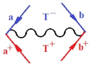
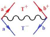
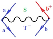
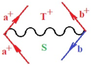
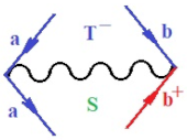
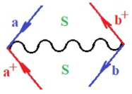
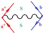
| Bondonic Diagram | Bondonic Symbol | Quantum Indices | |||
|---|---|---|---|---|---|
| Bonding Life-Lines of Creation–Annihilation | Total Spin | ||||
| “TT” Sector | |||||
 | TT+/+ | 2 | 2 | 1 | 1 |
 | TT−/− | 0 | 0 | −1 | −1 |
 | TT0/0 | −1 | −1 | 1 | −1 |
 | TT*/* | +1 | +1 | −1 | 1 |
| “TS” Sector | |||||
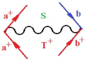 | TS+/0 | 2 | −1 | 1 | 0 |
 | TS0/+ | −1 | 2 | 1 | 0 |
 | TS−/* | 0 | +1 | −1 | 0 |
 | TS*/− | +1 | 0 | −1 | 0 |
| “ST” Sector | |||||
 | ST+/* | 2 | 1 | 0 | 1 |
 | ST0/− | −1 | 0 | 0 | −1 |
 | ST*/+ | +1 | 2 | 0 | 1 |
 | ST−/0 | 0 | −1 | 0 | −1 |
| “SS” Sector | |||||
 | SS0/* | −1 | +1 | 0 | 0 |
 | SS+/− | 2 | 0 | 0 | 0 |
 | SS−/+ | 0 | 2 | 0 | 0 |
 | SS*/0 | +1 | −1 | 0 | 0 |
| BONDONS-IN | BONDONS-OUT | ||||||
|---|---|---|---|---|---|---|---|
| Term “p” | ⊗ | Term “q” | = | Term “r” | ⊗ | Term “w” | |
| “TT” Sector | |||||||
| TT+/+ | ⊗ | TT−/− | = | SS−/+ | ⊗ | SS+/− | |
| TT+/+ | ⊗ | TT0/0 | = | TS0/+ | ⊗ | TS+/0 | |
| TT+/+ | ⊗ | TT*/* | = | ST*/+ | ⊗ | ST+/* | |
| TT−/− | ⊗ | TT0/0 | = | ST0/− | ⊗ | ST−/0 | |
| TT−/− | ⊗ | TT*/* | = | TS*/− | ⊗ | TS−/* | |
| TT0/0 | ⊗ | TT*/* | = | SS*/0 | ⊗ | SS0/* | |
| “TS” Sector | |||||||
| TS+/0 | ⊗ | TS0/+ | = | TT0/0 | ⊗ | TT+/+ | |
| TS+/0 | ⊗ | TS−/* | = | ST−/0 | ⊗ | ST+/* | |
| TS+/0 | ⊗ | TS*/− | = | SS*/0 | ⊗ | SS+/− | |
| TS0/+ | ⊗ | TS−/* | = | SS−/+ | ⊗ | SS0/* | |
| TS0/+ | ⊗ | TS*/− | = | ST+/+ | ⊗ | ST0/− | |
| TS−/* | ⊗ | TS*/− | = | TT*/* | ⊗ | TT−/− | |
 | ⊗ |  | = |  | ⊗ |  | |
| “ST” Sector | |||||||
| ST−/0 | ⊗ | ST0/− | = | TT0/0 | ⊗ | TT−/− | |
| ST−/0 | ⊗ | ST+/* | = | TS+/0 | ⊗ | TS−/* | |
| ST−/0 | ⊗ | ST*/+ | = | SS+/0 | ⊗ | SS−/+ | |
| ST0/− | ⊗ | ST+/* | = | SS+/− | ⊗ | SS0/* | |
| ST0/− | ⊗ | ST*/+ | = | TS+/− | ⊗ | TS0/+ | |
| ST+/* | ⊗ | ST*/+ | = | TT*/* | ⊗ | TT+/+ | |
 | ⊗ |  | = |  | ⊗ |  | |
| “SS” Sector | |||||||
| SS+/− | ⊗ | SS−/+ | = | TT−/− | ⊗ | TT+/+ | |
| SS+/− | ⊗ | SS0/* | = | ST0/− | ⊗ | ST+/* | |
| SS+/− | ⊗ | SS*/0 | = | TS*/− | ⊗ | TS+/0 | |
| SS−/+ | ⊗ | SS0/* | = | TS0/+ | ⊗ | TS−/* | |
| SS−/+ | ⊗ | SS*/0 | = | ST*/+ | ⊗ | ST−/0 | |
| SS0/* | ⊗ | SS*/0 | = | TT*/* | ⊗ | TT0/0 | |
 | ⊗ |  | = |  | ⊗ |  | |
| Methods | Results (eV) | |||
|---|---|---|---|---|
| Basis-A (3s2p1d) | Basis-B(4s3p1d) | Basis-C(4s3p1d) | Basis-D(5s4p1d) | |
| MRCCSD | 0.201 | 0.268 | 0.241 | 0.279 |
| MRCCSD+T*(3) | 0.190 | 0.254 | 0.228 | 0.265 |
| MRCCSD+T*−a(4) | 0.279 | 0.316 | 0.305 | 0.329 |
| MRCCSD+T*−b(4) | 0.246 | 0.290 | 0.274 | 0.303 |
| MRCCSD+T*b(4) | 0.253 | 0.294 | 0.280 | 0.307 |
| Experimental [84,86] | 0.437 ± 0.009 | |||
| Methods | Results (eV) | |||
|---|---|---|---|---|
| Basis-A (3s2p1d) | Basis-B (4s3p1d) | Basis-C (4s3p1d) | Basis-D (5s4p1d) | |
| MRCCSD | 0.356 | 0.421 | 0.399 | 0.435 |
| MRCCSD+T*(3) | 0.358 | 0.416 | 0.399 | 0.430 |
| MRCCSD+T*−a(4) | 0.455 | 0.499 | 0.491 | 0.515 |
| MRCCSD+T*−b(4) | 0.424 | 0.472 | 0.461 | 0.488 |
| MRCCSD+T*b(4) | 0.436 | 0.481 | 0.472 | 0.497 |
| Methods | Basis-A (3s2p1d) | Basis-B (4s3p1d) | Basis-C (4s3p1d) | Basis-D (5s4p1d) |
|---|---|---|---|---|
| Total Energy of Li2− (a.u.) | ||||
| MRCCSD | −14.9122 | −14.9148 | −14.9415 | −14.9430 |
| MRCCSD+T*(3) | −14.9123 | −14.9147 | −14.9415 | −14.9428 |
| MRCCSD+T*−a(4) | −14.9159 | −14.9177 | −14.9449 | −14.9459 |
| MRCCSD+T*−b(4) | −14.9147 | −14.9167 | −14.9438 | −14.9449 |
| MRCCSD+T*b(4) | −14.9152 | −14.9171 | −14.9442 | −14.9452 |
| Results (eV) | ||||
| MRCCSD | 0.225 | 0.291 | 0.267 | 0.303 |
| MRCCSD+T*(3) | 0.228 | 0.286 | 0.267 | 0.298 |
| MRCCSD+T*−a(4) | 0.324 | 0.369 | 0.360 | 0.384 |
| MRCCSD+T*−b(4) | 0.293 | 0.342 | 0.329 | 0.357 |
| MRCCSD+T*b(4) | 0.306 | 0.351 | 0.340 | 0.365 |
| Experimental [84,86] | 0.437 ± 0.009 | |||
| Methods | Results (eV) | |
|---|---|---|
| Basis-I | Basis-II | |
| MRCCSD | 1.81 | 2.05 |
| MRCCSD+T*(3) | 1.66 | 1.92 |
| MRCCSD+T*−a(4) | 1.81 | 2.09 |
| MRCCSD+T*−b(4) | 1.80 | 2.07 |
| MRCCSD+T*b(4) | 1.84 | 2.12 |
| CCSD (T) [87,88] | 1.79 | 2.18 |
| Experimental [84,86] | 2.15 ± 0.05 | |
| Methods | Results (eV) | |||
|---|---|---|---|---|
| Basis-A | Basis-B | Basis-C | Basis-D | |
| MRCCSD | 10.307 | 10.528 | 10.409 | 10.564 |
| MRCCSD+T*(3) | 10.217 | 10.416 | 10.321 | 10.450 |
| MRCCSD+T*−a(4) | 10.401 | 10.706 | 10.508 | 10.722 |
| MRCCSD+T*−b(4) | 10.382 | 10.680 | 10.487 | 10.696 |
| MRCCSD+T*b(4) | 10.366 | 10.675 | 10.474 | 10.691 |
| Experimental [84,86] | 10.64 | |||
Publisher’s Note: MDPI stays neutral with regard to jurisdictional claims in published maps and institutional affiliations. |
© 2021 by the authors. Licensee MDPI, Basel, Switzerland. This article is an open access article distributed under the terms and conditions of the Creative Commons Attribution (CC BY) license (https://creativecommons.org/licenses/by/4.0/).
Share and Cite
Basumallick, S.; Putz, M.V.; Pal, S. Three-Body Excitations in Fock-Space Coupled-Cluster: Fourth Order Perturbation Correction to Electron Affinity and Its Relation to Bondonic Formalism. Int. J. Mol. Sci. 2021, 22, 8953. https://doi.org/10.3390/ijms22168953
Basumallick S, Putz MV, Pal S. Three-Body Excitations in Fock-Space Coupled-Cluster: Fourth Order Perturbation Correction to Electron Affinity and Its Relation to Bondonic Formalism. International Journal of Molecular Sciences. 2021; 22(16):8953. https://doi.org/10.3390/ijms22168953
Chicago/Turabian StyleBasumallick, Suhita, Mihai V. Putz, and Sourav Pal. 2021. "Three-Body Excitations in Fock-Space Coupled-Cluster: Fourth Order Perturbation Correction to Electron Affinity and Its Relation to Bondonic Formalism" International Journal of Molecular Sciences 22, no. 16: 8953. https://doi.org/10.3390/ijms22168953
APA StyleBasumallick, S., Putz, M. V., & Pal, S. (2021). Three-Body Excitations in Fock-Space Coupled-Cluster: Fourth Order Perturbation Correction to Electron Affinity and Its Relation to Bondonic Formalism. International Journal of Molecular Sciences, 22(16), 8953. https://doi.org/10.3390/ijms22168953