Abstract
An experimental marine seismic source survey off the northwest Australian coast operated a 2600 cubic inch (41.6 l) airgun array, every 5.88 s, along six lines at a northern site and eight lines at a southern site. The airgun array was discharged 27,770 times with 128,313 pressure signals, 38,907 three-axis particle motion signals, and 17,832 ground motion signals recorded. Pressure and ground motion were accurately measured at horizontal ranges from 12 m. Particle motion signals saturated out to 1500 m horizontal range (50% of signals saturated at 230 and 590 m at the northern and southern sites, respectively). For unsaturated signals, sound exposure levels (SEL) correlated with measures of sound pressure level and water particle acceleration (r2 = 0.88 to 0.95 at northern site and 0.97 at southern) and ground acceleration (r2 = 0.60 and 0.87, northern and southern sites, respectively). The effective array source level was modelled at 247 dB re 1µPa m peak-to-peak, 231 dB re 1 µPa2 m mean-square, and 228 dB re 1 µPa2∙m2 s SEL at 15° below the horizontal. Propagation loss ranged from −29 to −30log10 (range) at the northern site and −29 to −38log10(range) at the southern site, for pressure measures. These high propagation losses are due to near-surface limestone in the seabed of the North West Shelf.
1. Introduction
Geophysical compressed-air (seismic) sources generate high-energy, low-frequency acoustic signals (most energy in band 10–100 Hz) with short rise times. The signals are produced by multiple airguns grouped in arrays, designed to direct maximum energy downward into the seabed. Travel time and character of signals reflected from density discontinuities in the seabed provide information on the layering of strata and potential hydrocarbon traps [1,2]. The frequencies produced by seismic sources fall within the hearing sensitivity of fishes [3,4], many invertebrates [5], reptiles [6,7], and marine mammals [8]. The combination of frequency spectra, intensity, and the extended duration of seismic survey operations (often weeks to months) can result in varying degrees of acute and chronic impacts on marine taxa [5,8,9,10,11,12,13,14,15,16]. These are primary considerations for regulators and industry in the approval and environmental management of exploration permits using seismic surveys.
Acoustic characteristics of an airgun array signal are dependent on the number, size, pressure, relative position, depth, and design of the airguns. Airgun arrays are typically spaced over 15–20 m along the array tow line and 10–20 m across it, containing multiple strings and a total of 12–40 individual airguns. Seismic survey array volumes range considerably, from < 1000 cubic inch (16.4 l) for shallow (<20 m) water operations, to 2500–5000 cui (41-81.9 l) for a ‘typical’ petroleum survey, up to in excess of 5000–6000 cui for deep geological imaging surveys in water depths of many thousands of metres [17].
For operational purposes and to estimate ranges of biological impact, airgun arrays are modelled to generate estimates of signal directionality, frequency content, and source level. The propagation of the signal from the array can be derived using the modelled source level combined with propagation loss to give an estimated received level with range, depth, and azimuth about the source. The estimated received level is used to identify significant exposure levels that may be experienced by fauna at given locations around the survey area [18]. Operational procedures and limitations can be put in place to mitigate the impact of the seismic signals on those fauna. However, propagation of sound energy in the ocean depends on the water depth, bathymetry profile along the propagation path, the geological layering of the seabed and the associated geo-acoustic properties, and the sound speed profile of the water column in vertical and, to a lesser extent, horizontal axes. Given the number of unknowns, significant measures are required at various distances and azimuths from the noise source to validate modelled exposure levels, particularly if the signals have to travel through environments of differing propagation losses [2,19,20,21]. Although the modelling step is usually implemented for mitigation of biological impacts these models are rarely validated.
Mitigation of the impact of an individual airgun signal or the accumulated exposure to multiple discharges on stationary or mobile fauna requires an understanding of: (1) what component of the acoustic signal animals respond to; (2) the threshold that elicits a response; and (3) how the intensity of this component varies with distance from the source. This is complicated by the fact that different marine taxa detect different components of the acoustic signal. For example, marine mammals [8] and some species of fish are sensitive to acoustic pressure, whereas all fishes are sensitive to sound-driven particle motion e.g., [3,22,23]. Marine invertebrates are predominantly sensitive to waterborne particle acceleration for animals that live above the seabed e.g., [24,25,26,27] or waterborne particle acceleration and ground acceleration for animals that live on or within it e.g., [15,16,28,29,30].
For a plane wave in the acoustic ‘far-field’, sound pressure and waterborne particle motion are related, and one can be estimated from the other. However, in the ‘near-field’, individual signals from a group of time-synchronized point sources (e.g., an array of airguns) will have travelled different distances and arrive at a receiver with different phases, leading to constructive and destructive interference. Far from the sources, the differences in distance travelled between signals originating from each source are minimal, waves arrive in phase, and intensity decreases with range (r) in the form of spherical spreading (i.e., 1/r2), assuming a free space [31]. The ranges at which this near- and far-field transition occurs are also dependent on interactions with boundaries, such as the sea surface, seafloor, or, to a lesser extent, mid-water boundary layers originating from sea water layering of density discontinuities. Thus, the distance at which a signal can be considered to be in the far-field is dependent on source geometry, frequency, water depth, substrate geo-acoustic parameters and changes in the physical water properties through the water column. Accurately quantifying these characteristics across a survey area prior to operation, is non-trivial.
Management of exposure levels generated by proposed seismic surveys would benefit from increased knowledge of how airgun signal metrics are related in the field and whether a single or handful of metrics can be used to evaluate the effects on multiple receptors. Sound exposure level (SEL) is one common metric used to quantify the energy levels, to assess their potential impact on fauna [18,32]. However, whether this provides an exposure measure appropriate for all taxa or types of biological impact has not been thoroughly explored. The measurement of pressure, particle motion, and ground motion energy levels from a seismic survey source are logistically and technically complex, and therefore uncommon. As a result, there is yet to be an empirically validated dataset that encompasses near- and far-fields to compare the three acoustic components and the numerous metrics that can be derived from them for a seismic source signal of commercial size. To explore these relationships, this study used calibrated acoustic pressure, particle motion, and ground motion measurements (including several co-located sensors), recorded during a seismic source exposure experiment that was operated under as-near-as-possible real-world (commercial survey) conditions off northwest Australia. In addition, we describe the technique used to derive measures of sound exposure for selected locations that were sampled for various biological impacts from the seismic operations.
2. Materials and Methods
Acoustic data were collected during a seismic exposure experiment to determine the responses of tropical demersal fishes and pearl oysters (Pinctada maxima) to a commercial-size geophysical compressed-air survey at two sites off the North West Shelf of Western Australia: a northern-shallow (≈15 m water depth lowest astronomical tide, LAT) and a southern-deep (≈55 m water depth LAT) one. For this paper, a line of seismic signals has been termed a ‘sail line’ and an individual airgun signal is the result of the airguns being ‘discharged’.
2.1. Study Sites
The northern site where the pearl oyster experiment occurred was located ≈ 40 km south southwest of Broome, in waters ranging between 10 and 25 m depth (Figure 1). A seafloor mapping study highlighted that the shoals to the northeast of the sail lines were 10–15 m deep at the time of the seismic survey, and covered by a fine layer of coarse sand overlying rock (limestone), with no sand at all in some areas (Supplementary Material, Figure S1). A total of six 23 km-long seismic sail lines were conducted in a roughly west to east direction (109°), starting 17 km west of the target location and finishing 6 km east. Water depths exceeded 40 m at the beginning of the sail line, in the west, and were 20–25 m deep at the opposite end of the sail line, in the east. At the western end, a 1–2 m deep layer of sand covered the limestone base, whereas at the eastern end this layer was thinner and over shoals the limestone was exposed.
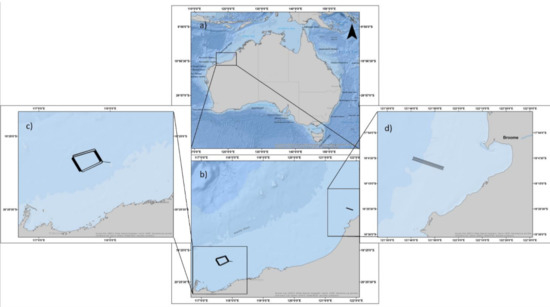
Figure 1.
Map of Australia (a) with expansion of northwest Australia (b). Additional expansions of the southern ((c); off Point Samson) and northern ((d); off Broome) sites and positions of seismic sail lines.
At the demersal fish experiment site in the south, the centres of the seismic sail lines were located ≈ 93 km north northeast of Cape Lambert. Sail lines were oriented on a 150° heading (Figure 1). The seafloor mapping study characterised the area as predominantly flat with a gentle slope from water depths of 55 m at the southern side of the site to depths of 80 m at the northern side, over a distance of 30 km (Supplementary Material, Figure S1). A combination of historical data from the region, towed video, and sediment grabs showed the seafloor was composed of a thin layer of coarse sand over a limestone base of relatively uniform hardness. Sessile biota (sponges, corals, sea whips) were present where the sand layer was at its thinnest (centimetres) or absent.
Pilot studies conducted with a single airgun provided provisional estimates of propagation losses greater than spherical spreading, with losses greater at the northern than the southern site (Supplementary Material, Figure S2).
2.2. Seismic Source and Operation
Two 2600 cui (41.61 l) airgun arrays were discharged alternately. Each array comprised two 12.5 m strings of guns (tow direction), each string comprised ten Sercel G Gun II airguns with each string spaced 5 m from the array central point (across tow direction, Supplementary Material, Figure S3, Tables S1 and S2). The arrays were towed 102 m astern of the vessel BGP Explorer, operated at 2000 psi (13.8 MPa), towed at 5 m depth and spaced 20 m to port and starboard of the vessel’s tow line. The arrays operated asynchronously at a mean 5.88 ± 0.004 s (95% CI) signal spacing (median 6 s) and median along-track distance of 12.5 m between signals. The modelled array beam pattern supplied by the contractor displayed little horizontal directionality (Supplementary Material, Figures S4 and S5).
At the northern site, one 23-km control sail line (airguns not operated) and six 23 km-long active sail lines were conducted with the first two active lines separated by 24 h and the following four active lines by 12 h. At the southern site, the seismic vessel operated eight control (eastern lines on Figure 1) and eight active (western) sail lines, every 12–13 h. The first two active sail lines were 25 km long and the last six, 20 km long. Control sail lines were 20 km (first two) or 15 km (last six) in length. All sail lines were operated with 500 m offsets between sequential lines, and all ran west to east.
The BGP Explorer provided: (1) airgun navigation data (*.p190 files for airgun signals with centre of source location only and UTC time to nearest second); (2) ships navigation data from a prescribed aerial; (3) ship specifications; (4) layout of ship, aerials, and source configuration; (4) seismic source details with modelled outputs in standard industry formats; and (5) daily logs.
2.3. Passive Acoustic Measurements
Three types of passive acoustic sensors were repeatedly deployed at different distances from the source to measure in-water acoustic pressure (underwater sound recorders, USR × 6) [33], particle motion (GeoSpectrum M20, GS-M20 × 2), and ground motion (three-axis geophones, GM × 2), during operation of the seismic sail lines (Table 1). Particle and ground motion measures were converted to provide measures of acceleration. Instruments were placed at different ranges around each site (Figure 2) for separate sail lines to quantify directionality in the beam pattern of the airgun arrays, account for sound propagation anomalies occurring due to variation in composition of the seabed, and to get a variety of closest-point-of approach (CPA) ranges. All USR and GM sensors were placed on the seafloor, whereas the GS-M20 sensor package was located 47 centimetres above the seabed, suspended from a tripod frame.

Table 1.
Instrument configurations, input signal tolerances, and expected operational ranges, including pre-amplifier gain (dB), the secondary gain (dB) applied in the digitizing electronics, and for the CMST-DSTO instruments: calculated maximum peak pressure (kPa and dB re 1 µPa), the maximum voltage at the hydrophone output.
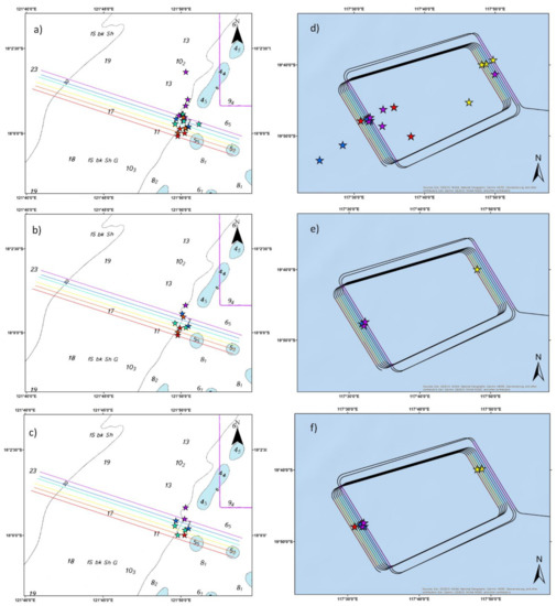
Figure 2.
Map of all acoustic sensor deployments for (a,d) pressure, (b,e) ground motion and (c,f) particle motion for the northern (left images) and southern (right images) experimental sites. Sensors notations (stars) are colour coded with the respective seismic sail lines they recorded. Seismic survey at the southern site was conducted as a racetrack design where the airgun array was only operated during sail lines at the western end of the track (coloured lines running north northwest to south southeast to the left of the images).
Multiple gain settings were used on instruments to measure airgun signals in the near-field without saturation and in the far-field without noise levels dropping into system electronic noise (see below). As the relationships between acoustic pressure, particle acceleration, and ground acceleration are complex in the near-field, deployments of the particle motion and ground motion sensors focussed on ranges of less than 2 km, whereas deployments of pressure sensors extended to ranges of > 30 km (Figure 2). All instruments used for measuring airgun signals collected 10-min samples running as frequently as possible (usually a 10 s gap between samples) at 4 kHz (GM, geophone and pressure), 8 kHz (USR), or 16 kHz (GS-M20, all channels) sample rates.
USRs were individually calibrated across all sampled frequencies using white noise of known level injected in series with the hydrophone [33]. Hydrophones used in the GM and USR instruments were Massa TR1025C or High Tech HTI U-90 (without in-built pre-amplifier), all individually calibrated with nominal sensitivity −198 to −196 dB re V/µPa. The white noise injection technique spans all frequencies and is particularly important for measuring airgun signals that have high intensities in low frequencies (< 400 Hz typically) where system impedance mismatches between hydrophone, pre-amplifier, and recording electronics will cause loss of sensitivity. The saved white noise was analysed to retrieve a frequency with gain curve (see Supplementary Material Figure S6 for an example calibration curve) which, when combined with hydrophone sensitivity, enabled calibration in the time or frequency domain, as required. USR clocks were synchronised with GPS transmitted time before each field trip and clock drift read at the field trip end using GPS transmitted time. Corrected clock times were then interpolated for the time in question to assist correct assignment of airgun signals between the BGP Explorer navigation logs and USR recording times.
Geophone measurements were taken using two USRs modified to include three-axis manufacturer-calibrated geophones, with an ION Geophysical, SM-6/U-B 10 Hz geophone in the vertical axis and two SM-6/H-B 10 Hz geophones aligned 90° apart in the horizontal plane. The instrument containing sensors was deployed flat with sensors coupled to the seabed. The frequency-dependent calibration response combined with the system gain provided calibration values for the system settings. The geophone sensors exhibited a noise floor of −15 dB re 1 ms−2, which was above ambient levels of ground acceleration. The GM instrument also included a pressure sensor. The GM pressure sensor pre-amplifier gain was fixed at 0 dB and the secondary gain set to either 0 or 20 dB dependent on the closest point of approach (CPA). The geophone channel gains were fixed.
Acoustic particle velocity was measured using two manufacturer-calibrated (generic sensor-type calibration curves, i.e., assumed to apply to all instruments of that type) GeoSpectrum GS-M20, three-axis particle velocity sensors connected to a JASCO AMAR logger. These sensors (x and y horizontal and z vertical) were mounted in a tripod frame set on the seabed with the sensor hanging from the apex of the frame ≈ 47 cm above the seafloor (inbuilt tilt sensors confirmed the mooring had been deployed in an upright position). The x, y, and z channel phase responses of the GS-M20 velocity sensor were included in the calibration process. The GS-M20 sensor package had a 20 dB fixed gain that could not be modified and a secondary gain at the AMAR recorder of 0–18 dB, set depending on expected CPA. The calibration specifications (particle velocity sensitivity and phase or pressure sensor sensitivity, respectively) were combined with the system gain and the AMAR analogue to digital electronics rail (5 V) to the *.wav file format (± 1), to return calibrated waveforms (ms−1 or Pa) in the time domain (method defined below). The GeoSpectrum-AMAR units allowed for clocks to be synchronised to laptop times (UTC) and the drift read post deployments. The GS-M20 data included roll, pitch, yaw, and magnetic declination that when corrected to the horizontal and vertical plane gave the sensor tilt in three-axis and calibrated compass headings.
Airgun signals have high peak amplitudes close to the source (< 1 km) that can result in the sensor voltage saturating (or overloading) the recording system electronics if the input voltage at the pre-amplifier output is too high. Saturated signals can simply be clipped (i.e., the top of the signal cut off above some voltage threshold) or the electronics can produced artefacts that may persist for much longer than the input signal. Diode protection for the pre-amplifier and digitizing electronics are present in some systems to limit this effect. The diodes begin to reduce the input signal at a lower voltage than the maximum voltage they allow through, thus biasing signals close to the protection threshold. For saturated signals the correct received airgun level cannot be calculated.
We used eight instrument configurations to measure airgun signals. Each configuration had an optimal range bracket at which it could be deployed from the airgun array, based on the system dynamic range (lowest to highest peak signal levels) and noise floor (level the signal will be detected above background or system self-noise). For each configuration, we calculated the maximum signal peak pressures that could be tolerated (Table 1), assuming a hydrophone sensitivity of −196 dB re V/µPa and a voltage threshold before diode protection started at levels above or below 2.3/−2.3 V, respectively, for the USR instruments. These details were not calculated for the GS-M20, which only had secondary gain, as precise details of the system electronics, particularly any voltage protection applied were not available.
2.4. Signal Metrics
There are numerous metrics or signal characteristics that may be important in driving responses from marine fauna to a ‘noise’ signal [18,27,28,32,34]. The response thresholds for these metrics are likely species-specific and possibly vary with life function or condition [35]. Although the three acoustic pressure components and indeed many of the metrics are correlated, their relationships are not necessarily consistent or linear as the signal propagates away from the source [36]. It is probable that different metrics are applicable to different forms of an animal’s response, such as propensity for physiological impact where the mechanical response and so forces driving an organ are important or behavioural responses where the neurological interpretation of signals are important. Sound exposure level (SEL) is the most common metric for quantifying impulsive airgun signals with practical techniques to determine this and other metrics described by McCauley et al. [18], Madsen [32], or defined in ISO standard 18405-2017 [37]. Multiple signal parameters have been derived here from pressure, particle acceleration and ground acceleration. Metrics include SEL, mean-square sound pressure level (SPL), peak-to-peak sound pressure level (P-P), peak values of an airgun signal’s horizontal and vertical vectors of particle acceleration (differentiated particle velocity), maximum magnitude of the airgun signal’s particle acceleration vector (the 3-axis vectors combined into a single magnitude with two angles per time point) and the same peak ground acceleration vector and magnitude components (Table 2). Note, as per ISO 18405-2017 the acceleration values used here are “field” quantities which do not involve any averaging or root mean squared values being calculated. On page 4, Section 3.1.2.11, Note 3, ISO 18405:2017 defines “sound particle acceleration” with units specified as ms−2 [37]. These units have been used throughout the paper. The conversion of acceleration units to decibels is listed in ISO 18405:2017 as where a is the value and the reference value used, which is stated as 1 µms−2 for acceleration.
Table 2.
Description of acoustic metrics quantified for individual discharges of the 2600 cui airgun array.
In addition to the above metrics, McCauley and Duncan [34] speculated that it is the high positive peak value immediately followed by a high negative peak value received over a short time-period (often referred to as ‘jerk’) that causes physical trauma in some taxa. This jerk is observed in the pressure and three-axis motion component of the signal. The aspects which are important in this measure are the positive and negative peak values and the time between these peaks. To test this, we created a unit from the airgun signal pressure waveform, which divides the sum of absolute values of maximum and minimum pressures within the airgun signal waveform, by the time between these peaks (dB re 1 µPa∙s−1, Table 2). For simplicity in calculation and future replication, we used maximum and minimum values experienced across the defined time window of the airgun signal. Here, this metric has been called peak pressure gradient (PPG). At low received airgun signal levels, the PPG values are low and random in distribution as the received signals have no clear peak values and the time between peaks is random. Once a clear positive peak immediately followed by a high negative peak value appears in the waveform the PPG measure stabilizes and rapidly increases as the time between peaks drops. An increase in positive or negative peak values experienced increases the PPG value, as does a shorter time between the two peaks. In contrast, differentiating the pressure waveform as suggested by some can provide the slope or rate of change of the pressure signal, but it does not correctly account for the time between maximum positive and minimum negative peaks.
2.5. Airgun Signal Processing
Airgun pressure signals were extracted and analysed for each metric by the following steps:
- Identify samples in a data set with airgun signals by aligning seismic navigation logs with sea-noise sample start and end times;
- Load a sample, and down-sample to 4 kHz to match the geophone pressure channel and high-pass filter at 2 Hz;
- Display the full sample waveform (10 min, volts using a 5–100 Hz band-pass filtered signal) and spectrogram (10–500 Hz displayed) for each recording that included airgun array signals;
- Identify the ‘leading edge’ of each airgun signal (band-pass filtered) by applying a voltage threshold (specific to a sample, which is dependent on the range of the recording site to the airgun source), combined with a minimum time separation (5 s, based on BGP Explorer navigational log data) between consecutive airgun signals;
- Delete any identified airgun signals which had overlapping ‘noise’ sources;
- Remove each identified signal from the high-pass only filtered sample (volts at this stage) by extracting the signal from 4 s before to 4 s after the identified time of leading edge;
- Calibrate the signal by obtaining the fast Fourier transform (FFT) of the airgun signal voltage waveform (frequency resolution of ≈ 0.12 Hz, or 32,768 points using 4 kHz sampling frequency), multiplying the real FFT part by the amplitude correction for that frequency, then converting back to a calibrated signal with an inverse FFT (see McCauley et al. [19], for further detail);
- Calculate the level of each metric including those in Table 2, for each signal;
- Calculate power spectra of each extracted signal;
- Save extracted airgun signals, level metrics, start and end time of airgun signal (as given by times for 5% and 95% of signal energy to pass), a flag for if the signal had saturated or not and the power spectra.
The airgun signal times were used to extract and analyse the three-axis geophone and particle velocity (GS-M20) values using the appropriate data set. Each particle velocity channel for an airgun signal was checked for overload and flagged for the channel if the saved *.wav volts exceeded ±0.98 V (to allow for some diode protection). The geophone channels did not overload. The geophone and particle velocity signals were extracted similarly to the pressure signals and as for the pressure signals, calibrated in the time domain using their respective gain with frequency curves (independent sensor types) and for the GS-M20 data, including the appropriate sensor phase calibrations (correcting the real and imaginary part of the FFT for amplitude and phase response, respectively, before the inverse FFT was calculated).
For all airgun signals, the arrival time was aligned with the seismic navigation data and the airgun signal identified in the recordings, after assuming a sound speed and accounting for range between discharged and received signal. Once the airgun signal was defined the source to receiver geometry was established (horizontal range and angle from array tow direction to receiver).
All saturated airgun signals were removed in all analysis. Saturated signals were defined by using the flag from the saved data or identifying ranges below which a particular data set had attained a plateau and removing all values below this range.
To compare different metrics, co-located signals from various sensors were found. Linear regression models were used to assess correlation between selected metrics and investigate how one metric such as SEL, predicted other metrics at the individual airgun signal level (i.e., same airgun signal measured by different sensors) using unsaturated signals.
To estimate received levels for each airgun signal at biological sampling sites:
- The airgun strings were symmetrical along the centre of their towlines. Therefore, any potential beam pattern was considered similar on the port and starboard sides, and port and starboard measurements were collated;
- Measurements for each metric were gridded into a 2D space of horizontal range and azimuth (angle of receiver from tow direction) using linear interpolation and a constant sized grid spacing. No smoothing was applied in this step, data were linearly interpolated;
- The resulting 2D grid was interpolated for missing values within the data matrixes (this was only required for ≈ 30 points, for some metrics);
- The edges of the gridded matrix were populated for ranges greater or less than the maximum or minimum measured range, respectively, for any particular azimuth, or for azimuths less than or greater than as measured at a particular range, using a variety of techniques, specific to each metric;
- All airgun signal received levels at ranges greater than ≈ 30 km (depending on the metric) were set to the ambient noise level as it was not possible to analyse these received airgun signal levels. This was because at this range signals were within 2 dB of ambient noise levels and had smeared in time so that no recognisable peak occurred.
Linear regression was applied to the measured data using the equations:
where RL is received level in the appropriate metric, a, b, and c are constants derived from the fit, and R is horizontal range of source to receiver (m). Correlation coefficients (r2) were calculated for each fit. An alternative technique for defining trends of received level with range was to calculate statistics of dB values for the appropriate metric in logarithmic range bins, with bin centres and widths defined by one-third octave bands:
where bc is centre of bin (m), N is an increasing integer value, bl is the lower range limit for that bin-centre, and bu is the upper range limit (m). The value N is iterated to include the maximum range to be encountered.
Horizontal range (great circle path between source and receiver), rather than slant range (the direct path between the source near the surface and the receiver at the seabed), was used to determine propagation loss across the experimental sites. The distance at which slant vs. horizontal range would be significant at each site was estimated by applying spherical spreading from the known array source level at a given elevation to calculate horizontal received level and slant range received level, accounting for water depth, array depth and maximum tidal excursion over the experimental period. The two estimated received level values for that range were then compared. The maximum tidal excursion during the survey period at the northern site was 5.3 m. When combined with the water depth and the mean lowest astronomical tide (LAT) in the area, less 5 m for the source depth, a 1 dB difference between slant and horizontal range occurred at 70 m horizontal range. At ranges > 70 m, this error declined rapidly. The equivalent range at the southern site, for a 1 dB difference, was ≈ 120 m horizontal range, beyond which the difference again dropped rapidly. For signals recorded at shorter ranges, measurement plots of logarithmic range with received level would appear more consistent if slant range was used. However: (1) inter-discharge variability in SEL has been shown to range between 1 and 3 dB [38] and the different received level estimates for slant and horizontal ranges fell below 3 dB at horizontal ranges of approximately 10 and 30 m for the northern and southern sites, respectively; and (2) all levels at biological sites were calculated using horizontal range (provided a consistent range type was used this made no difference to exposure estimates).
3. Results
3.1. Measurements
Over the experimental exposure period, 39 instruments were deployed 108 times on 58 moorings. From the airgun source navigation data, 27,770 active airgun signals were logged, 14,227 at the northern site and 13,543 at the southern site. The mean discharge interval was 5.9 s (median 6 s, 95%CI ± 0.0044 s, n = 27,769). Of these airgun signals, 128,313 unsaturated pressure signals were measured from different instruments, from horizontal ranges of 12 m (almost directly below the array at northern site) to 20.3 km. At the northern site, 58,402 pressure signals were analysed and 69,911 at the southern site. Although all measurements included the pressure signal, 17,832 included three-axis ground-borne geophone measures (8688 and 9144 at the northern and southern sites, respectively) and 38,907 included three-axis particle velocity measurements (19,160 and 19,747 at the northern and southern sites, respectively). Matched geophone and particle velocity measurements were available for 877 airgun signals (505 and 372 at the northern and southern sites, respectively), with the geophone and particle velocity sensors within 30–50 m of each other and on the seabed (geophone) or 47 cm above the seabed (particle motion). Histograms of ambient noise levels for each metric at the time of the seismic survey can be found in Supplementary Material, Figure S7 and received SELs for an example sail line at each site are shown in Figures S8 and S9.
Using the source model of Duncan [2] the 2600 cui airgun array was estimated to have effective source levels of: (1) 252 dB re 1 µPa m peak-to-peak pressure, 234 dB re 1 µPa2 m2 mean-square pressure, and 228 dB re 1 µPa2∙m2s SEL, directly below the array; and (2) 247 dB re 1 µPa m peak-to-peak pressure, 231 dB re 1 µPa2 m mean-square pressure, and 228 dB re 1 µPa2∙m2s SEL at 15° below the horizontal (more relevant to longer range horizontal source level than the higher levels directly below the array). The maximum measured levels and the horizontal ranges at which they were measured, can be found in Table 3. Within a few hundred m of the array most energy emitted occurred with uniform spectral density between 2 and 100 Hz with almost all energy < 1000 Hz (Figure 3). The passage of the BGP Explorer past a USR, during a seismic sail line, illustrated the frequency-dependent propagation of the signal showing that with range, almost all energy remained under ≈ 100 Hz, at the northern site, while at the southern site, the highest energy was under 100 Hz with peaks around 10 Hz and 50 Hz (Figure 4). The ’waisting’ with frequency evident at each site on Figure 4) is due to the limestone seabed preferentially attenuating certain frequencies [38]. Energy > 100 Hz propagated only short distances (Figure 4). A Lloyd’s mirror interference pattern, typical of a point source varying with increasing range was more clearly visible at the southern site where energy propagated further (compare Figure 4a with 4b).
Table 3.
Maximum levels measured at the northern and southern sites, and the horizontal range at which they occurred for peak-to-peak pressure level (P-P), sound exposure level (SEL), mean-square sound pressure level (SPL), pressure peak-gradient (PPG), seabed ground acceleration (maximum horizontal and vertical vectors and magnitude), and particle acceleration (maximum horizontal and vertical vectors and magnitude) levels, as defined in Table 2.
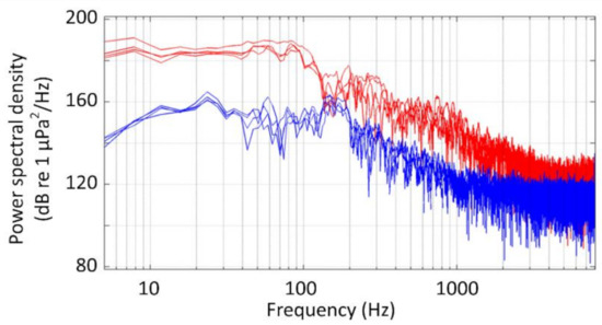
Figure 3.
Pressure power spectra measured almost directly underneath airgun array (red) and at 190 m (blue).
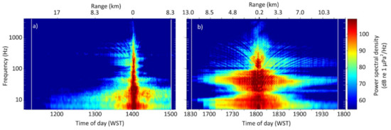
Figure 4.
Power spectral density of pressure signals from the airgun array as recorded by a USR throughout an individual seismic sail line operated at the northern ((a), closest point of approach, ≈12 m horizontal range, 18 September) and southern ((b), closest point of approach, ≈190 m horizontal range, 21 September) sites. The white lines mark the start and end of airgun operations along the seismic line.
3.2. Saturated Signals
The proportion of saturated signals to total airgun array signals measured illustrated how the different instruments and gain settings performed with increasing range from the airgun array (Figure 5b). The pressure channel of the GS-M20 using the lowest secondary gain setting of 0 dB saturated at ranges between 300 and 700 m. Particle motion signals recorded by the GS-M20 began saturating at 1.2 and 1.5 km from the source at the northern and southern sites, respectively (Figure 5a), and increased in the proportion of saturated signals to the closest ranges at which recordings were taken. At ranges of 230 and 590 m (northern and southern sites, respectively), 50% of the particle motion measures were saturated. The ground motion accelerometers’ signals were not saturated at any range. However, at long ranges (or under low level ambient conditions) the sensor response fell into the system electronic noise floor and the sensors did not provide ambient level ground acceleration.
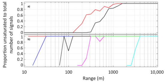
Figure 5.
Proportion of unsaturated to total signals within logarithmic horizontal range brackets for: (a) particle motion at the northern (red) and southern (black) sites; and (b) pressure only for USR instruments with pre-amp/secondary gain (dB) settings of −40/0 (red), −20/0 (blue), 0/0 (black), 0/20 (magenta), 20/0 (green) and 20/20 (cyan). The expected working ranges for each sensor can be found in Table 1.
3.3. Received Levels with Range
At the northern and southern sites received levels of all metrics decreased with range at rates greater than spherical spreading and did so at a greater rate at the northern (shallower), compared to southern (deeper) site (Figure 6). The trends shown for each metric averaged in logarithmic range bins (Figure 7, bin ranges defined by Equations (3)–(5) clearly highlighted the poorer sound propagation conditions at the northern site. Mean levels for five metrics at 250, 500, and 1000 m displayed up to 17 dB difference between the sites (Table 4). The confidence limits in averaging in the logarithmic range bins were low at each site, with the mean error < 0.7 dB at either site. At short-range (low hundreds of metres), the trends with range shown on Figure 7 converged for all metrics.

Figure 6.
Received levels of the airgun array signal with range for the southern (black) overlaid with northern (red) sites for: (a) peak-to-peak pressure level; (b) sound exposure levels; (c) mean-square sound pressure levels; (d) maximum magnitude ground acceleration; (e) and maximum magnitude particle acceleration. Mean values at each range (all data) interpolated along log10(range) (continuous blue line), together with the 95% confidence intervals (dotted blue lines) are shown along with the fitted curve (Equation (2)) using all data as the red curve.

Figure 7.
Received levels of the airgun array signal averaged in logarithmic range bins with horizontal range for the northern (blue) and southern (red) sites for peak-to-peak pressure level (a), sound exposure level (b), mean-square sound pressure level (c), maximum magnitude ground acceleration (d), and maximum magnitude particle acceleration (e) levels.
Table 4.
Received levels with 95% confidence limits (±) and sample size (n), for peak-to-peak pressure level (P-P), sound exposure level (SEL), mean-square sound pressure level (SPL), maximum magnitude ground acceleration (MxMGA), and maximum magnitude particle acceleration (MxMPA), with logarithmic range bin centred at 250, 500, and 1000 (m), for the two sites.
Coefficients for the linear regression curves formed for each of the five metrics using Equation (2), showed the propagation loss coefficient ranged between −17 and −31 at the northern site and −16 and −38 across all metrics at the southern site (Table 5). In comparison, when Equation (1) was applied at short ranges and Equation (2) was applied at long ranges (minimum and maximum ranges for each metric defined in Table 6 and Table 7), short-range propagation loss decreased significantly at the southern site (compare column ‘a’ values for the southern site between Table 6 and Table 7).
Table 6.
Parameters for fits to metrics for northern and southern sites at short-range using horizontal-range limited curve fitting (Equation (1)), with correlation coefficient (r2) for each fit and the maximum range used in the curve fitting. Abbreviations defined in Table 2.
Table 7.
Parameters for fits to metrics for northern and southern sites at long horizontal range using Equation (2), with correlation coefficient (r2) for each fit and the minimum range used in the curve fitting. Abbreviations defined in Table 2.
There was no major evidence of horizontal beam pattern of the airgun array or localised sound propagation variation within an experimental area in any of the measured metrics (Figure 8, Figure 9 and Figure 10). All metrics displayed comparatively uniform propagation loss away from the source across all azimuths (0° to 180°), with the exception of PPG (compare received levels with range from the source for Figure 8, Figure 9 and Figure 10 with that of Figure 8d). Although PPG displayed a general decline in received levels with increasing range, there were patches of sudden changes in received levels at all ranges and azimuths. The spatial propagation plots suggested a weak beam pattern was present (semi-circular ‘step’ declines in level with range when plotted as azimuth against range in a cartesian, rather than polar plot), however, these were in fact unavoidable artefacts of the sampling design, created by the multiple straight line passes of the seismic vessel past stationary recording sensors, (areas of high-density sampling; Figure 8, Figure 9 and Figure 10).
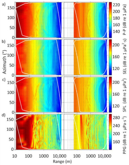
Figure 8.
Peak-to-peak pressure levels (a), sound ex-posure levels (b), mean-square sound pressure levels (c) and pressure peak gradient (d) for the northern (N = left) and southern (S = right) sites, shown as a function of logarithmic horizontal range and azimuth (y-axis, o) from tow direction (assumed array symmetrical, 0° is ahead). The white lines encapsulate measured data bounds. Gridding used linear interpolation.
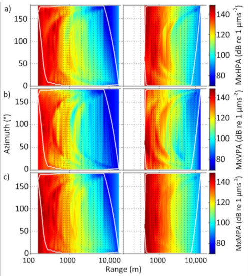
Figure 9.
Maximum values of horizontal (a), vertical (b), and magnitude (c) particle acceleration levels for the northern (N = left) and southern (S = right) sites, shown as a function of logarithmic horizontal range and azimuth (y-axis, °) from tow direction (assumed array symmetrical, 0° is ahead). The white lines encapsulate measured data bounds. The colour axes are common across panels. Gridding used linear interpolation.

Figure 10.
Maximum values of horizontal (a), vertical (b), and magnitude (c), ground acceleration levels for the northern (N = left) and southern (S = right) sites, shown as a function of logarithmic horizontal range and azimuth (y-axis, °) from tow direction (assumed array symmetrical, 0° is ahead). The white lines encapsulate measured data bounds. The colour axes are common across panels. Gridding used linear interpolation.
3.4. Correlation of Airgun Signal Metrics
SEL was strongly correlated with P-P and SPL, with the correlation coefficients for SEL/P-P and SEL/SPL, 0.88 and 0.95, respectively, at the northern site, both 0.97 at the southern site, and 0.94 and 0.95, respectively, when using all data combined (Table 8). When comparing SEL with maximum magnitude of ground acceleration and particle acceleration, these correlations dropped to 0.60 and 0.64, respectively, at the northern site, 0.87 and 0.93, respectively, at the southern site, and 0.74 and 0.77, respectively, for all data combined (Table 8). Particle acceleration and ground acceleration showed strong correlation, particularly at the southern site (0.87), though also at the northern site (0.64), and overall (0.80, all data). In the units used, dB re 1 µms−2, ground acceleration was given by particle acceleration 47 cm above the seabed, minus ≈ 23 dB (Figure 11). In general, correlations were stronger at the southern, deeper site, than the northern site (Figure 11, Table 8). SEL did a poor job of predicting PPG.
Table 8.
Statistics of linear fits for the correlations shown including first and second coefficients of the linear regression fit (a and b), correlation coefficient, standard error (SE) and the 95% confidence error of the first coefficient of the linear fit. Abbreviations are defined in Table 2.
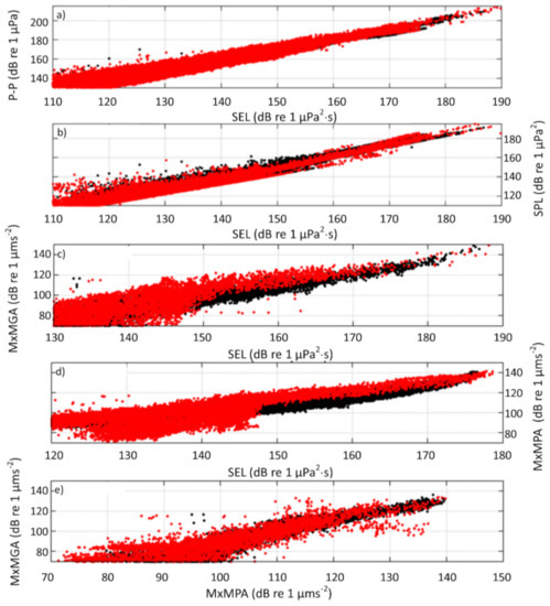
Figure 11.
Relationship between pairs of metrics, for the southern site (black dots) overlaid with the northern site (red dots) for sound exposure level against peak-to-peak pressure level (a), sound exposure level against mean-square sound pressure level (b), SEL against magnitude of ground acceleration (c), sound exposure level against magnitude of particle acceleration (d), and magnitude of particle acceleration against magnitude of ground acceleration (e).
4. Discussion
Received levels recorded in this study showed that the exposure levels experienced from the 2600 cui source operated at both sites were similar to those likely to be experienced by fauna around typical commercial surveys under similar conditions [19,39]. This comprised energy at frequencies that would be detected by many marine taxa [40,41]. Propagation loss through the experimental areas were typical of environments with comparable water depths (50–70 m) uniform bathymetry and a similar seafloor composition (a thin layer of sand over limestone pavement [2]). The relatively high propagation losses at our study sites were due to the interaction with the underlying or exposed limestone seabed compared with thicker layers of sand elsewhere [2]. This limestone seabed is typical of continental shelf waters across southern and western Australia into the far northwest [19]. The lack of directionality in the beam pattern combined with comparatively uniform depth and seabed substrate allowed robust estimates of exposure levels at biological sampling sites to be predicted for the two experimental areas with high levels of confidence, based on the correlation coefficients found for different metrics.
Sound exposure level was strongly correlated with mean-square sound pressure level (r2 = 0.95) and peak-to-peak pressure levels (r2 = 0.94). SEL was also correlated (though to a lesser degree) with the maximum magnitudes of particle acceleration (r2 = 0.77) and maximum magnitude of ground acceleration (r2 = 0.74) when using all data. The correlation of SEL and ground or particle acceleration improved at the more uniform southern site (r2 > 0.87). The relationships between pressure and ground acceleration metrics were valid across all ranges as unsaturated recordings were collected even at ranges closest to the source. However, although some measures of particle acceleration in the near-field did not overload and remain correlated with SEL, relationships involving particle acceleration in the near-field < 500 m could not be fully assessed due to the saturation of >50% of measured signals. The correlation between SEL and ground acceleration was weaker at the shallower northern site (r2 = 0.60) than at the deeper southern site (r2 = 0.87). The reasons for this were not explored though are likely due to the northern site having a more diverse range of seabed types(cm to m of sand over limestone or no sand and the instrument lying on limestone, compared with tens cm to m of sand at the southern site).
In this situation, harder seafloors will dampen the ground acceleration. The results highlighted a strong correlation between particle acceleration near the seafloor and seabed ground acceleration (r2 = 0.80 when using all data).
These results imply that SEL is a good proxy for other conventional pressure metrics, particle acceleration and ground acceleration, when assessing the impact of noise on fauna at horizontal ranges of more than ≈250 and ≈600 m (northern and southern sites, respectively) with a similar source for sites with similar depths and geophysical characteristics (e.g., sound speed profile and seafloor types).
The metric PPG correlated relatively poorly with other metrics and was not predicted well by SEL. This was believed to be due to the time between peaks at low level (SEL) signals. At low received levels, the peaks arrived randomly within the signal causing large natural variability in PPG values. Even at a short range, with low to modest received airgun signal levels the time between peaks was highly variable, causing differences in the PPG measure. This metric was introduced as a simple measure of airgun signal ‘jerk’, which McCauley and Duncan [34] speculated generates physiological damage in invertebrates. To reduce variation, the measure may need to be more complex in its derivation, for example, by constraining the measures to consecutive peaks instead of the time between maximum positive and negative peaks within the signal. The application of PPG cannot be assessed until measured biological impacts have been correlated and compared to other more standard metrics (i.e., SEL). It may be that the variation observed in PPG around an airgun array correlates with physiological trauma in some marine fauna.
The empirically measured correlations between metrics in this study show that where environmental management is assessing the impact of impulsive acoustic signals, such as those from seismic surveys, at ranges of 100 s of m and greater (i.e., acoustic transition- and far-fields) then SEL may be used as a proxy for other metrics. This minimizes the need for acquiring particle or ground acceleration data unless there are specific concerns regarding benthic, sessile, or species of low-mobility.
Supplementary Materials
The following are available online at https://www.mdpi.com/article/10.3390/jmse9060571/s1, Figure S1: Map of sonar backscatter from a multibeam survey of the southern-deep site (left images) and the northern-shallow site (right images). Still images captured from towed video at points indicated on the map show examples of seabed corresponding to different levels of backscatter and benthic organisms (mostly sponges and gorgonians) within zones., Figure S2: Sound exposure levels with range of a 150 cui airgun towed and discharged every 60 s along one transect at the northern site (red dots) and two transects conducted at the southern site (blue–offshore side and black dots–inshore side), Figure S3: Airgun (black squares) positions and sizes for the 2600 cui arrays towed by BGP Explorer where size of marker has been scaled to reflect the relative volume of the airgun and arrow denotes direction of travel, Figure S4: Modelled (PGS Nucleus model) source signal waveform (a) and relative power spectral density (b) for the far-field signature of the 2600 cui airgun array signal (5 m source depth, 41.8 bar m primary pressure). Red line in (b) marks the -6 dB limit. Images supplied by Exploiter PTE. LTD, Figure S5: Modelled (PGS Nucleus) airgun array signal directivity patterns for (a) horizontal plane directivity at 60 Hz, (b) vertical plane along-track directivity at 50 Hz, and (c) vertical plane across-track directivity at 50 Hz. Images supplied by Exploiter PTE. LTD, Figure S6: Example of system gains with frequency response for USRs from the white noise injection calibration, Figure S7: Distribution of ambient noise levels for peak-to-peak pressure level (a), sound exposure level (b), mean-square sound pressure level (c), PPG (d), maximum horizontal particle acceleration (e), maximum vertical particle acceleration (f) and maximum magnitude of particle acceleration (g) at the northern (left columns) and southern (right columns) sites, Figure S8: Sound exposure levels with range for a seismic sail line operated at the northern site on 18th September 2018 ((a) and (b)) by USRs positioned at various distances from the sail line. Coloured dots relate to the USR datasets from the recording positions shown in (c) using the respective colours from a) and b), Figure S9: Sound exposure levels with range for a seismic sail line operated at the southern site on 23rd September 2018 ((a) and (b)) by USRs positioned at various distances from the sail line. Coloured dots relate to the USR datasets from the recording positions shown in (c) using the respective colours from a) and b). Periods where an increasing number of guns were operated prior to the start of the seismic sail line (i.e., the ‘ramp-up’) are highlighted, Table S1: Configuration of each 2600 cui array, where X is the across-track axis (negative to port and positive to starboard direction, referenced to the centreline of the vessel) and Y is the along-track axis (positive to forward, referenced to the forward guns), Table S2: Characteristics of seismic vessel operations at each experimental site, Table S3: Details of the source vessel, MV BGP Explorer. Ancilliary data [42].
Author Contributions
Conceptualization, M.J.G.P., R.D.M. and M.G.M.; methodology, formal analysis, writing—original draft preparation, visualization, R.D.M. and M.J.G.P.; writing—review and editing, M.J.G.P., R.D.M. and M.G.M.; funding acquisition, M.G.M. All authors have read and agreed to the published version of the manuscript.
Funding
This work was conducted as part of the North West Shoals to Shore Program, which is proudly supported by Santos as part of the company’s commitment to better understand WA’s marine environment.
Institutional Review Board Statement
The experiment during which this data was collected was conducted according to the guidelines of the Declaration of Helsinki, and approved by the Ethics Committee of the University of Western Australia (RA/3/100/159, 5/6/2018).
Informed Consent Statement
Not applicable.
Data Availability Statement
The acoustic data supporting this study is available on request from the Australian Institute of Marine Science.
Acknowledgments
The authors would like to acknowledge the crew of the RV Solander who facilitated the deployment of all acoustic sensors. The authors would also like to thank the anonymous reviewers for their time to consider the manuscript and useful comments to improve the content.
Conflicts of Interest
The authors declare no conflict of interest. The funders participated in a stakeholder workshop during the development of the experimental design of the overall program. This workshop was attended by collaborators and stakeholders including: AIMS, Curtin University, University of Tasmania, Western Australia’s Department of Primary Industry and Regional Development, WA Fishing Industry Council, commercial fishers, members of the WA pearling industry, geophysical contractors, members of the petroleum industry, as outlined in the Supplemental Material. The funders had no role in the collection, analyses, or interpretation of data; in the writing of the manuscript, or in the decision to publish the results.
References
- Gisiner, R.C. Sound and marine seismic surveys. Acoust. Today 2016, 12, 10–18. [Google Scholar]
- Duncan, A.J. Airgun Arrays for Marine Seismic Surveys-Physics and Directional Characteristics. In Proceedings of the Acoustics 2017, Perth, Australia, 19–22 November 2017; p. 10. [Google Scholar]
- Popper, A.N.; Hawkins, A.D.; Fay, R.R.; Mann, D.A.; Bartol, S.; Carlson, T.J.; Coombs, S.; Ellison, W.T.; Gentry, R.L.; Halvorsen, M.B. ASA S3/SC1. 4 TR-2014 Sound Exposure Guidelines for Fishes and Sea Turtles: A Technical Report Prepared by ANSI-Accredited Standards Committee S3/SC1 and Registered with ANSI; Springer: Berlin/Heidelberg, Germany, 2014. [Google Scholar]
- Ladich, F.; Fay, R.R. Auditory evoked potential audiometry in fish. Rev. Fish Biol. Fish. 2013, 23, 317–364. [Google Scholar] [CrossRef]
- Carroll, A.; Przeslawski, R.; Duncan, A.J.; Gunning, M.; Bruce, B. A critical review of the potential impacts of marine seismic surveys on fish & invertebrates. Mar. Pollut. Bull. 2017, 114, 9–24. [Google Scholar]
- Martin, K.J.; Alessi, S.C.; Gaspard, J.C.; Tucker, A.D.; Bauer, G.B.; Mann, D.A. Underwater hearing in the loggerhead turtle (Caretta caretta): A comparison of behavioral and auditory evoked potential audiograms. J. Exp. Biol. 2012, 215, 3001–3009. [Google Scholar] [CrossRef] [PubMed]
- Chapuis, L.; Kerr, C.C.; Collin; Hart, N.S.; Sanders, K.L. Underwater hearing in sea snakes (Hydrophiinae): First evidence of auditory evoked potential thresholds. J. Exp. Biol. 2019, 222. [Google Scholar] [CrossRef] [PubMed]
- Southall, B.L.; Finneran, J.J.; Reichmuth, C.; Nachtigall, P.E.; Ketten, D.R.; Bowles, A.E.; Ellison, W.T.; Nowacek, D.P.; Tyack, P.L. Marine mammal noise exposure criteria: Updated scientific recommendations for residual hearing effects. Aquat. Mam. 2019, 45, 125–232. [Google Scholar] [CrossRef]
- Slabbekoorn, H.; Dalen, J.; de Haan, D.; Winter, H.V.; Radford, C.; Ainslie, M.A.; Heaney, K.D.; van Kooten, T.; Thomas, L.; Harwood, J. Population-level consequences of seismic surveys on fishes: An interdisciplinary challenge. Fish Fish. 2019, 20, 653–685. [Google Scholar] [CrossRef]
- Paxton, A.B.; Taylor, J.C.; Nowacek, D.P.; Dale, J.; Cole, E.; Voss, C.M.; Peterson, C.H. Seismic survey noise disrupted fish use of a temperate reef. Mar. Pol. 2017, 78, 68–73. [Google Scholar]
- Bruce, B.; Bradford, R.; Foster, S.; Lee, K.; Lansdell, M.; Cooper, S.; Przeslawski, R. Quantifying fish behaviour and commercial catch rates in relation to a marine seismic survey. Mar. Environ. Res. 2018, 140, 18–30. [Google Scholar] [CrossRef]
- Davidsen, J.G.; Dong, H.G.; Linné, M.; Andersson, M.H.; Piper, A.; Prystay, T.S.; Hvam, E.B.; Thorstad, E.B.; Whoriskey, F.; Cooke, S.J.; et al. Effects of sound exposure from a seismic airgun on heart rate, acceleration and depth use in free-swimming Atlantic cod and saithe. Cons. Physiol. 2019, 7. [Google Scholar] [CrossRef]
- Kavanagh, A.S.; Nykänen, M.; Hunt, W.; Richardson, N.; Jessopp, M.J. Seismic surveys reduce cetacean sightings across a large marine ecosystem. Sci. Rep. 2019, 9, 19164. [Google Scholar] [CrossRef]
- Hubert, J.; Neo, Y.Y.; Winter, H.V.; Slabbekoorn, H. The role of ambient sound levels, signal-to-noise ratio, and stimulus pulse rate on behavioural disturbance of seabass in a net pen. Behav. Proc. 2020, 170, 103992. [Google Scholar] [CrossRef] [PubMed]
- Day, R.D.; McCauley, R.D.; Fitzgibbon, Q.P.; Hartmann, K.; Semmens, J.M. Seismic air guns damage rock lobster mechanosensory organs and impair righting reflex. Proc. R. Soc. B. 2019, 286, 20191424. [Google Scholar] [CrossRef] [PubMed]
- Day, R.D.; Fitzgibbon, Q.P.; McCauley, R.D.; Hartmann, K.; Semmens, J.M. Lobsters with pre-existing damage to their mechanosensory statocyst organs do not incur further damage from exposure to seismic air gun signals. Envir. Poll. 2020, 267, 115478. [Google Scholar] [CrossRef]
- Gisiner, R.; Harper, S.; Livingston, E.; Simmen, J. Effects of Sound on the Marine Environment (ESME): An underwater noise risk model. IEEE J. Ocean. Eng. 2006, 31, 4–7. [Google Scholar] [CrossRef]
- McCauley, R.D.; Fewtrell, J.; Duncan, A.J.; Jenner, C.; Jenner, M.-N.; Penrose, J.D.; Prince, R.I.T.; Adhitya, A.; Murdoch, J.; McCabe, K. Marine seismic surveys: Analysis and propagation of airgun signals; and effects of exposure on humpback whales, sea turtles, fishes and squid. In (Anon) Environmental Implications of Offshore Oil and Gas Development in Australia: Further Research; Australian Petroleum Production Exploration Association: Canberra, Australia, 2003; pp. 364–521. Available online: www.cmst.curtin.edu.au\publications (accessed on 11 May 2021).
- McCauley, R.D.; Duncan, A.J.; Gavrilov, A.N.; Cato, D.H. Transmission of marine seismic survey, air gun array signals in Australian waters. In Proceedings of the Acoustics 2016, Brisbane, Australia, 9–11 November 2016. [Google Scholar]
- Dunlop, R.A.; Noad, M.J.; McCauley, R.D.; Kniest, E.; Slade, R.; Paton, D.; Cato, D.H. The behavioural response of migrating humpback whales to a full seismic airgun array. Proc. Roy. Soc. B Biol. Sci. 2017, 284, 20171901. [Google Scholar] [CrossRef] [PubMed]
- Morris, C.; Cote, D.; Martin, B.; Kehler, D. Effects of 2D seismic on the snow crab fishery. Fish. Res. 2018, 197, 67–77. [Google Scholar] [CrossRef]
- Popper, A.N.; Hastings, M. The effects of anthropogenic sources of sound on fishes. J. Fish Biol. 2009, 75, 455–489. [Google Scholar] [CrossRef]
- Popper, A.; Hawkins, A.; Halvorsen, M. Anthropogenic sound and fishes. In Report by ICF for Washington State Department of Transportation; Research Office: Washington, DC, USA, 2019; Available online: https://www.wsdot.wa.gov/research/reports/fullreports/891-1.pdf (accessed on 22 May 2021).
- Meyer-Rochow, V.B.; Penrose, J.D. Sound production by the western rock lobster Panulirus longipes (Milne Edwards). J. Exp. Mar. Biol. Ecol. 1976, 23, 191–209. [Google Scholar] [CrossRef]
- André, M.; Kaifu, K.; Sole, M.; van der Schaar, M.; Akamatsu, T.; Balastegui, A.; Sanchez, A.M.; Castell, J.V. Contribution to the Understanding of Particle Motion Perception in Marine Invertebrates. In The Effects of Noise on Aquatic Life II. Advances in Experimental Medicine and Biology; Popper, A., Hawkins, A., Eds.; Springer: New York, NY, USA, 2016; Volume 875. [Google Scholar] [CrossRef]
- Montgomery, J.C.; Radford, C.A. Marine bioacoustics. Curr. Biol. 2017, 27, R502–R507. [Google Scholar] [CrossRef]
- Popper, A.N.; Hawkins, A.D. The importance of particle motion to fishes and invertebrates. J. Acoust. Soc. Amer. 2018, 143, 470–488. [Google Scholar] [CrossRef] [PubMed]
- Day, R.D.; McCauley, R.D.; Fitzgibbon, Q.P.; Semmens, J.M. Assessing the Impact of Marine Seismic Surveys on Southeast Australian Scallop and Lobster Fisheries; FRDC Report, Project No 2012/008; University of Tasmania: Hobart, Australia, 2016; p. 167. Available online: https://frdc.com.au/project/2012-008 (accessed on 22 May 2021).
- Day, R.D.; McCauley, R.D.; Fitzgibbon, Q.P.; Hartmann, K.; Semmens, J.M. Scallops shaken following seismic surveys: Exposure to air gun signals affects mortality, physiology and behaviour. Glo. Chan. Biol. 2017. [Google Scholar] [CrossRef]
- Day, R.D.; McCauley, R.D.; Fitzgibbon, Q.P.; Hartmann, K.; Semmens, J.M. Exposure to seismic air gun signals causes physiological harm and alters behavior in the scallop Pecten Fumatus. Proc. Nat. Acad. Sci. USA 2017, 114. [Google Scholar] [CrossRef]
- Erbe, C. Underwater Acoustics: Noise and the Effects on Marine Mammals a Pocket Handbook, 3rd ed.; JASCO Applied Sciences: Brisbane, Australia, 2013. [Google Scholar]
- Madsen, P. Marine mammals and noise: Problems with root mean square sound pressure levels for transients. J. Acoust. Soc. Amer. 2005, 117, 3952–3957. [Google Scholar] [CrossRef]
- McCauley, R.D.; Thomas, F.; Parsons, M.J.G.; Erbe, C.; Cato, D.H.; Duncan, A.J.; Gavrilov, A.N.; Parnum, I.M.; Salgado-Kent, C.P. Developing an Underwater Sound Recorder: The Long and Short (Time) of It…. Acoust. Aus. 2017, 45, 301–311. [Google Scholar] [CrossRef]
- McCauley, R.D.; Duncan, A.J. How do Impulsive Marine Seismic Surveys Impact Marine Fauna and How Can We Reduce Such Impacts? In Proceedings of the Acoustics 2017, Perth, Australia, 20 November 2017; 4p. [Google Scholar]
- Harding, H.R.; Gordon, T.A.C.; Wong, K.; McCormick, M.I.; Simpson, S.D. Condition-dependent responses of fish to motorboats. Biol. Lett. 2020, 16, 20200401. [Google Scholar]
- Urick, R.J. Principles of Underwater Sound, 3rd ed.; Peninsula Publishing Los Atlos: California, CA, USA, 1983. [Google Scholar]
- International Organization for Standardization. Underwater Acoustics—Terminology; IOS: Geneva, Switzerland, 2017. [Google Scholar]
- Duncan, A.J.; Gavrilov, A.N.; McCauley, R.D.; Parnum, I.M.; Collis, J.M. Characteristics of sound propagation in shallow water over an elastic seabed with a thin cap-rock layer. J. Acoust. Soc. Am. 2013, 134, 207–215. [Google Scholar] [CrossRef] [PubMed]
- Greene, C.R., Jr. Characteristics of marine seismic survey sounds in the Beaufort Sea. J. Acoust. Soc. Am. 1988, 83, 2246. [Google Scholar] [CrossRef]
- Duarte, C.M.; Chapuis, L.; Collin, S.P.; Costa, D.P.; Devassy, R.P.; Eguiluz, V.M.; Erbe, C.; Gordon, T.A.C.; Halpern, B.S.; Harding, H.R.; et al. The Ocean Soundscape of the Anthropocene. Science 2021, 371, 581. [Google Scholar] [CrossRef]
- Mooney, T.A.; Di Iorio, L.; Lammers, M.; Lin, T.H.; Nedelec, S.L.; Parsons, M.J.G.; Radford, C.A.; Urban, E.; Stanley, J. Listening forward: Approaching marine biodiversity assessments using acoustic methods. R. Soc. Open Sci. 2020, 7, 201287. [Google Scholar] [CrossRef]
- Whiteway, T.G. Australian Bathymetry and Topography Grid, June 2009. In Geoscience Australia Record 2009/21; Geoscience Australia: Canberra, Australia, 2009; p. 46. [Google Scholar]
Publisher’s Note: MDPI stays neutral with regard to jurisdictional claims in published maps and institutional affiliations. |
© 2021 by the authors. Licensee MDPI, Basel, Switzerland. This article is an open access article distributed under the terms and conditions of the Creative Commons Attribution (CC BY) license (https://creativecommons.org/licenses/by/4.0/).