
Deep-Learning-Based Classification of Cyclic-Alternating-Pattern Sleep Phases


Abstract
:1. Introduction
- A fully automatic classifier of cyclic alternating pattern (CAP) signals, based on a computationally efficient neural network, which therefore can be implemented on-device.
- Extensive experiments demonstrate state-of-the-art performance on a public CAP benchmark database, classifying its A and B phases using only a single EEG signal.
- An ablation study was conducted to assess the impact of different time-frequency representations, segment sizes, and types of data augmentation.
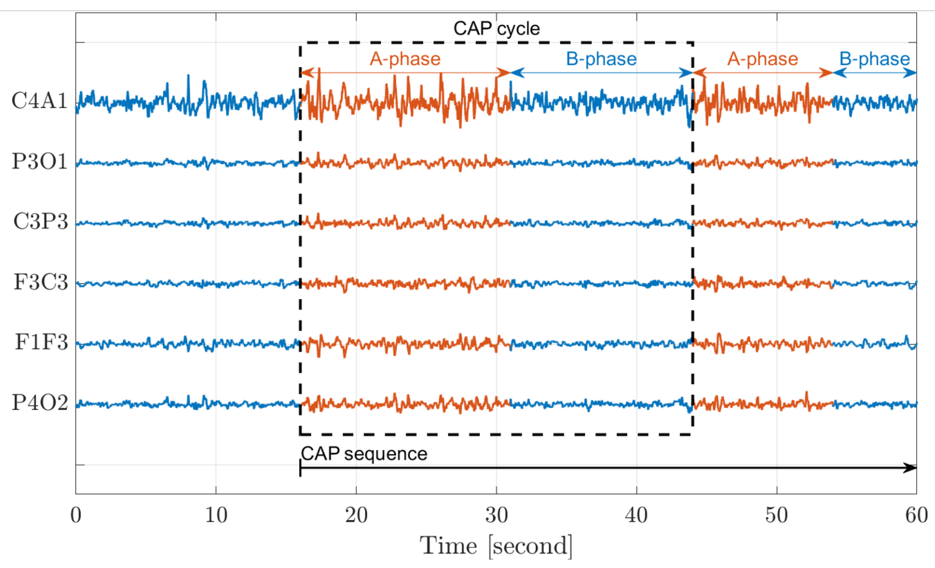
2. Background
- A1 is dominated by slow varying waves (low frequencies, 0.5 Hz–4 Hz) with a high amplitude about the typical background, B-phase.
- A3 is characterized by increasing in frequency (8 Hz–12 Hz) along with decreasing in the amplitude.
- A2 is a combination of both A1 and A3.
3. Related Work
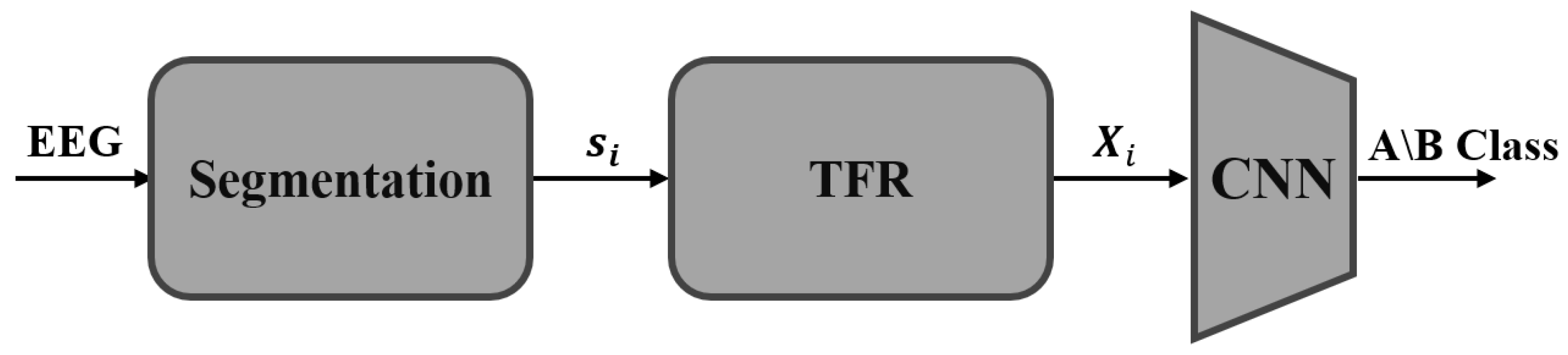
4. Proposed Method
- Context—Incorporating contextual information of the signal to make the prediction more analogous to the human diagnosis, which inherently involves close vicinity analysis.
- CAP prior knowledge—Utilizing the distinct features of the A-phase events, which are characterized by higher energy levels and high-frequency spectral content compared to the B-phase background.
- Deep learning—Employing a CNN-based architecture as a classifier to leverage the CNN’s high-performance capabilities.
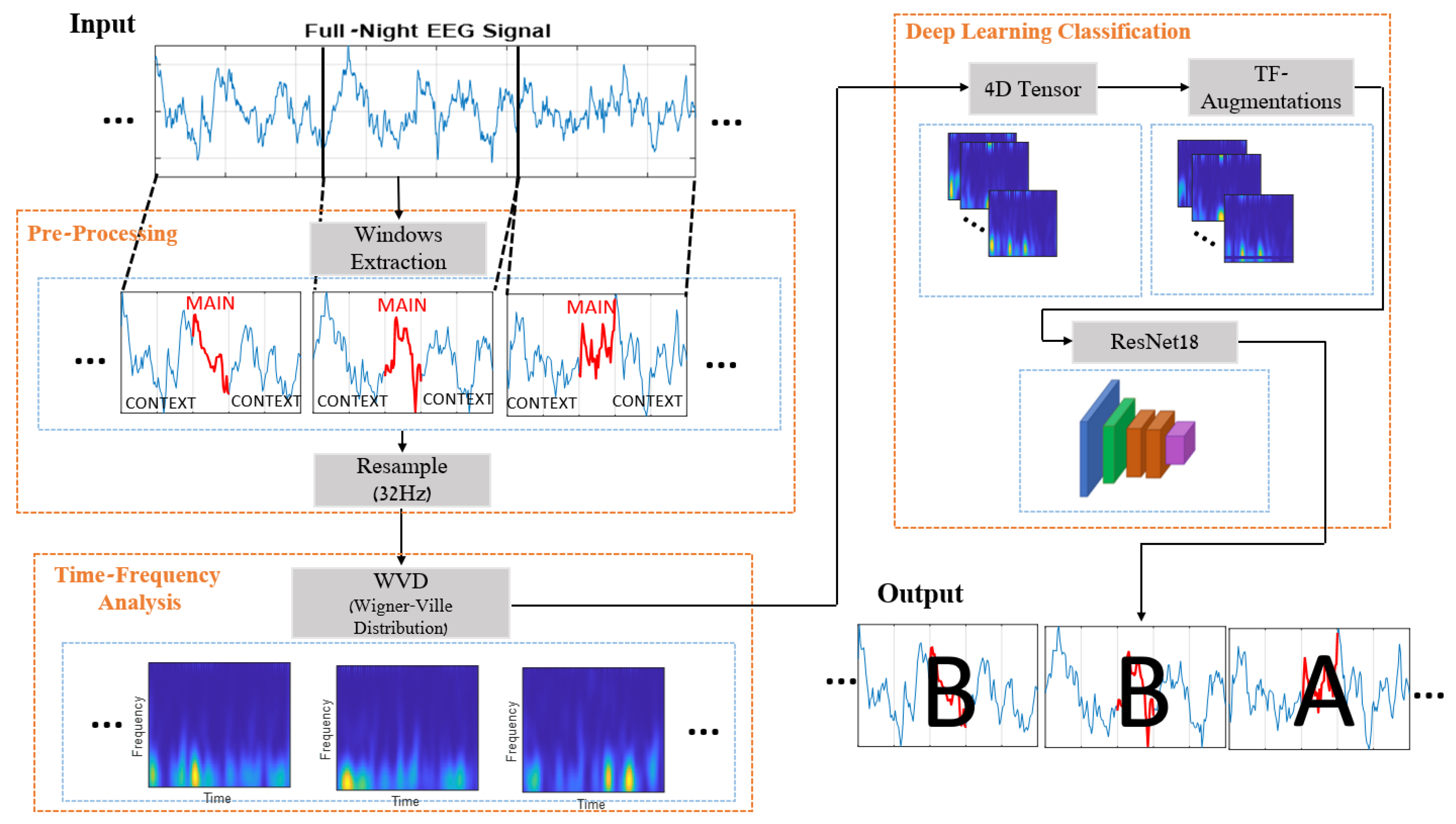
4.1. Pre-Processing
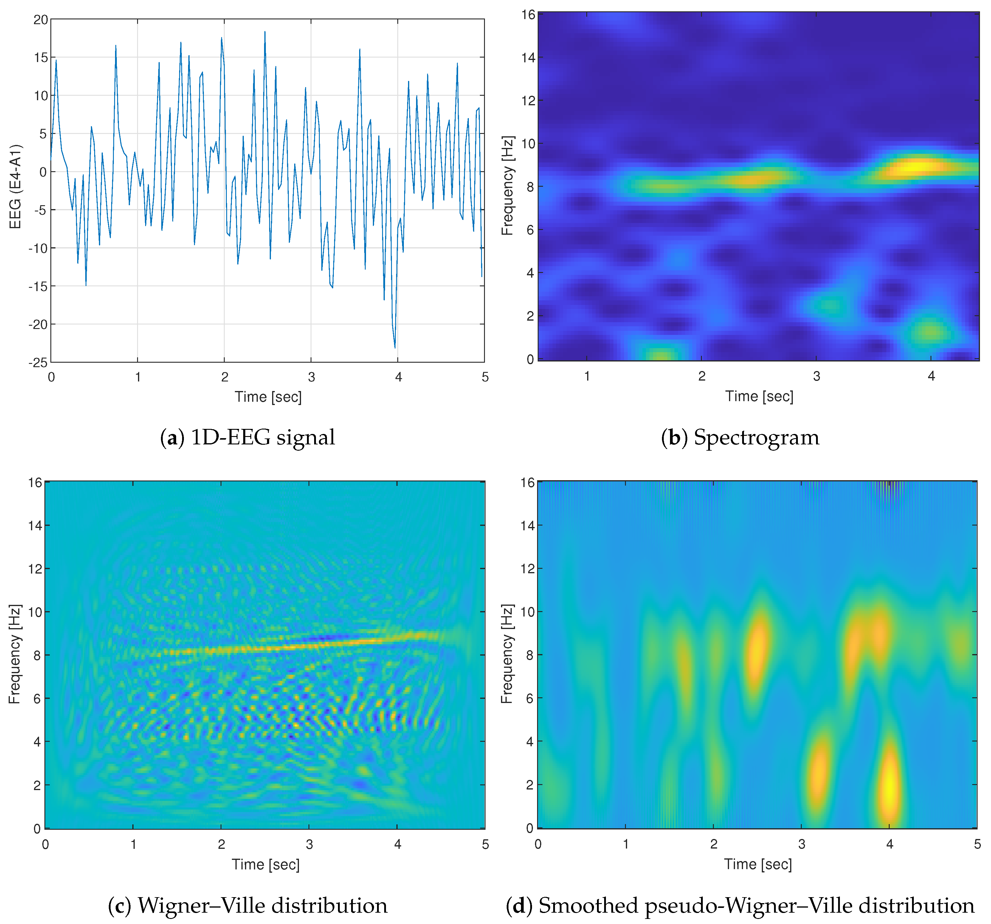
4.2. Time-Frequency Analysis
4.2.1. Spectrogram (SPEC)
4.2.2. Wigner–Ville Distribution (WVD)
4.2.3. Smoothed Pseudo Wigner–Ville Distribution (SPWVD)
4.3. Deep Learning Architecture
4.3.1. Model
4.3.2. Normalization
4.3.3. Augmentations
- Time-shifts: We employed random time-shifts by applying horizontal random cropping to the training data samples. The cropping was restricted to the horizontal axis, i.e., the time domain, to maintain the spectral information of the signals and preserve the distinction between the different phases of CAP, which differ significantly in their spectral characteristics.
- Time-frequency augmentations (TF-Aug.): A specialized selection of augmentations was utilized to characterize the time-frequency representations effectively. These augmentations were repeatedly applied to each data sample before inputting the neural network. The selected augmentations are:
- Noise: Additive white Gaussian noise (AWGN) with a uniformly distributed standard deviation. Adding noise was specified in [48] as an appropriate and effective augmentation for EEG signals
- Gaussian blur: The time-frequency images were blurred using a Gaussian kernel. This augmentation was randomly applied to the input samples with a probability of , meaning that approximately half of the images underwent blurring.
- SpecAugment [49]: A commonly used method for augmenting spectrograms and other time-frequency representations, typically for speech recognition tasks. The augmentation is primarily based on applying random masks to certain frequency bands and time steps in the spectrogram. In this study, we randomly blocked bands up to 5% of image width for time and 3% of image height for frequency.
- Crop and Resize: To imitate extended temporal CAP events, we randomly cropped the images vertically and then resized them back to their original size, slightly stretching the temporal duration of CAP events.
5. Materials and Methods
5.1. Database Description
5.2. Performance Measures
5.3. Dataset Creation
6. Numerical Results
- The influence of utilizing various time-frequency representations as input to the classifiers.
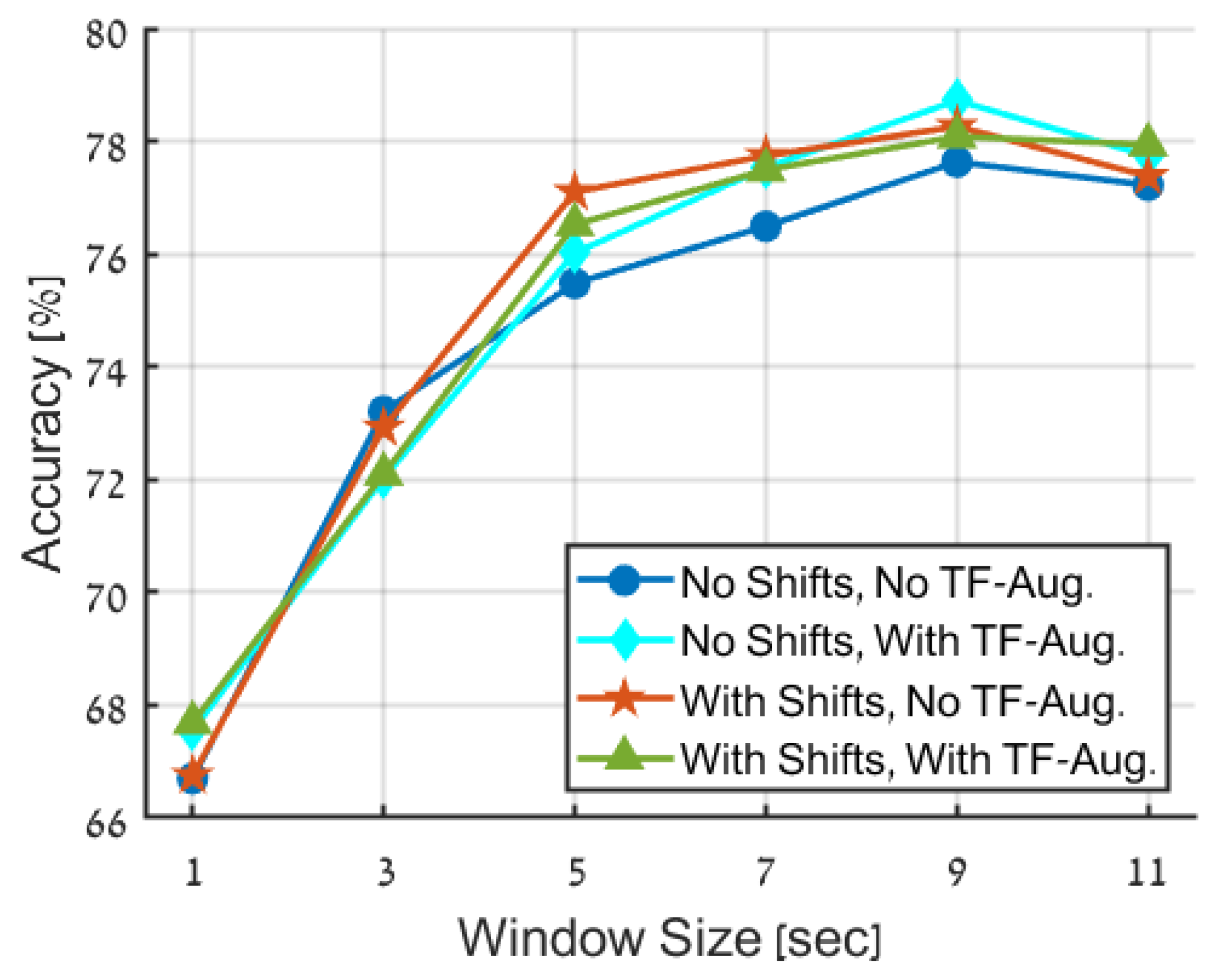
- The impact of incorporating the EEG signal context information by using segments with an increased duration.
- The determination of appropriate data augmentations strategies for analyzing EEG signals within the proposed framework.
- TF-augmentation: TF-augmentations are applied solely. As described above, these augmentations are designed to maintain the time-frequency structure.
- Random time-shifts: In this case, the original dataset is augmented by incorporating random time shifts into its samples.
- TF-augmentations and random time-shifts: Both TF-augmentations and random time-shifts are applied to the dataset.
A-Phase Detection
7. Conclusions
Author Contributions
Funding
Institutional Review Board Statement
Informed Consent Statement
Data Availability Statement
Conflicts of Interest
Abbreviations
| CAP | Cyclic alternating pattern |
| EEG | Electroencephalography |
| CNN | Convolutional neural network |
| TFR | Time-frequency representation |
| STFT | Short-time Fourier transform |
| WVD | Wigner–Ville distribution |
| CAPSLPDB | Cap Sleep Database |
| AASM | American Academy of Sleep Medicine |
| REM | Rapid eye movement |
| PSD | Power spectral density |
| LDA | Linear discriminant analysis |
| SVM | Support vector machines |
| DL | Deep learning |
| LSTM | Long short-term memory |
| SPWVD | Smoothed pseudo-Wigner–Ville distribution |
| SPEC | Spectrogram |
| CT | Cross-terms |
| AT | Auto-terms |
| AF | Ambiguity function |
| TF | Time-frequency |
| SGD | Stochastic gradient descent |
| AWGN | Additive white Gaussian noise |
| EOG | Electrooculogram |
| EMG | Electromyogram |
| ACC | Accuracy |
| TPR | True-positive rate |
| RE | Renyi entropy |
| BOWFB | Biorthogonal wavelet filter bank |
Appendix A

References
- Terzano, M.G.; Parrino, L. The cyclic alternating pattern (CAP) in human sleep. In Handbook of Clinical Neurophysiology; Elsevier: Amsterdam, The Netherlands, 2005; Volume 6, pp. 79–93. [Google Scholar]
- Terzano, M.G.; Parrino, L.; Sherieri, A.; Chervin, R.; Chokroverty, S.; Guilleminault, C.; Hirshkowitz, M.; Mahowald, M.; Moldofsky, H.; Rosa, A.; et al. Atlas, rules, and recording techniques for the scoring of cyclic alternating pattern (CAP) in human sleep. Sleep Med. 2001, 2, 537–554. [Google Scholar] [CrossRef] [PubMed]
- Parrino, L.; Ferri, R.; Bruni, O.; Terzano, M.G. Cyclic alternating pattern (CAP): The marker of sleep instability. Sleep Med. Rev. 2012, 16, 27–45. [Google Scholar] [CrossRef] [PubMed]
- Terzano, M.G.; Parrino, L. Clinical applications of cyclic alternating pattern. Physiol. Behav. 1993, 54, 807–813. [Google Scholar] [CrossRef] [PubMed]
- Mendonca, F.; Fred, A.; Shanawaz Mostafa, S.; Morgado-Dias, F.; Ravelo-García, A.G. Automatic detection of a phases for CAP classification. In Proceedings of the 7th International Conference on Pattern Recognition Applications and Methods, Funchal, Portugal, 16–18 January 2018. [Google Scholar]
- Mendonca, F.; Fred, A.; Mostafa, S.S.; Morgado-Dias, F.; Ravelo-Garcia, A.G. Automatic detection of cyclic alternating pattern. Neural Comput. Appl. 2022, 34, 11097–11107. [Google Scholar] [CrossRef]
- Mariani, S.; Bianchi, A.M.; Manfredini, E.; Rosso, V.; Mendez, M.O.; Parrino, L.; Matteucci, M.; Grassi, A.; Cerutti, S.; Terzano, M.G. Automatic detection of A phases of the Cyclic Alternating Pattern during sleep. In Proceedings of the 2010 Annual International Conference of the IEEE Engineering in Medicine and Biology, Buenos Aires, Argentina, 31 August–4 September 2010; pp. 5085–5088. [Google Scholar]
- Mariani, S.; Grassi, A.; Mendez, M.O.; Parrino, L.; Terzano, M.G.; Bianchi, A.M. Automatic detection of CAP on central and fronto-central EEG leads via Support Vector Machines. In Proceedings of the 2011 Annual International Conference of the IEEE Engineering in Medicine and Biology Society, Boston, MA, USA, 30 August–3 September 2011; pp. 1491–1494. [Google Scholar]
- Mariani, S.; Manfredini, E.; Rosso, V.; Grassi, A.; Mendez, M.O.; Alba, A.; Matteucci, M.; Parrino, L.; Terzano, M.G.; Cerutti, S.; et al. Efficient automatic classifiers for the detection of A phases of the cyclic alternating pattern in sleep. Med. Biol. Eng. Comput. 2012, 50, 359–372. [Google Scholar] [CrossRef] [PubMed]
- Mariani, S.; Grassi, A.; Mendez, M.O.; Milioli, G.; Parrino, L.; Terzano, M.G.; Bianchi, A.M. EEG segmentation for improving automatic CAP detection. Clin. Neurophysiol. 2013, 124, 1815–1823. [Google Scholar] [CrossRef] [PubMed]
- Sharma, M.; Patel, V.; Tiwari, J.; Acharya, U.R. Automated characterization of cyclic alternating pattern using wavelet-based features and ensemble learning techniques with eeg signals. Diagnostics 2021, 11, 1380. [Google Scholar] [CrossRef] [PubMed]
- Dhok, S.; Pimpalkhute, V.; Chandurkar, A.; Bhurane, A.A.; Sharma, M.; Acharya, U.R. Automated phase classification in cyclic alternating patterns in sleep stages using Wigner–Ville distribution based features. Comput. Biol. Med. 2020, 119, 103691. [Google Scholar] [CrossRef]
- Sharma, M.; Bhurane, A.A.; Acharya, U.R. An expert system for automated classification of phases in cyclic alternating patterns of sleep using optimal wavelet-based entropy features. Expert Syst. 2022, e12939. [Google Scholar] [CrossRef]
- Loh, H.W.; Ooi, C.P.; Dhok, S.G.; Sharma, M.; Bhurane, A.A.; Acharya, U.R. Automated detection of cyclic alternating pattern and classification of sleep stages using deep neural network. Appl. Intell. 2022, 52, 2903–2917. [Google Scholar] [CrossRef]
- Hartmann, S.; Baumert, M. Automatic a-phase detection of cyclic alternating patterns in sleep using dynamic temporal information. IEEE Trans. Neural Syst. Rehabil. Eng. 2019, 27, 1695–1703. [Google Scholar] [CrossRef] [PubMed]
- You, J.; Ma, Y.; Wang, Y. GTransU-CAP: Automatic labeling for cyclic alternating patterns in sleep EEG using gated transformer-based U-Net framework. Comput. Biol. Med. 2022, 147, 105804. [Google Scholar] [CrossRef] [PubMed]
- Sejnowski, T.J. The Deep Learning Revolution; MIT Press: Cambridge, MA, USA, 2018. [Google Scholar]
- Voulodimos, A.; Doulamis, N.; Doulamis, A.; Protopapadakis, E. Deep learning for computer vision: A brief review. Comput. Intell. Neurosci. 2018, 2018. [Google Scholar] [CrossRef] [PubMed]
- Deng, J.; Dong, W.; Socher, R.; Li, L.J.; Li, K.; Fei-Fei, L. Imagenet: A large-scale hierarchical image database. In Proceedings of the 2009 IEEE Conference on Computer Vision and Pattern Recognition, Miami, FL, USA, 20–25 June 2009; pp. 248–255. [Google Scholar]
- Ariav, I.; Cohen, I. An end-to-end multimodal voice activity detection using wavenet encoder and residual networks. IEEE J. Sel. Top. Signal Process. 2019, 13, 265–274. [Google Scholar] [CrossRef]
- Gu, J.; Wang, Z.; Kuen, J.; Ma, L.; Shahroudy, A.; Shuai, B.; Liu, T.; Wang, X.; Wang, G.; Cai, J.; et al. Recent advances in convolutional neural networks. Pattern Recognit. 2018, 77, 354–377. [Google Scholar] [CrossRef]
- Madan, R.; Agrawal, D.; Kowshik, S.; Maheshwari, H.; Agarwal, S.; Chakravarty, D. Traffic Sign Classification using Hybrid HOG-SURF Features and Convolutional Neural Networks. In Proceedings of the International Conference on Pattern Recognition Applications and Methods, Prague, Czech Republic, 19–21 February 2019; pp. 613–620. [Google Scholar]
- Chen, Y.; Yang, X.; Zhong, B.; Pan, S.; Chen, D.; Zhang, H. CNNTracker: Online discriminative object tracking via deep convolutional neural network. Appl. Soft Comput. 2016, 38, 1088–1098. [Google Scholar] [CrossRef]
- Zhang, C.; Yao, C.; Shi, B.; Bai, X. Automatic discrimination of text and non-text natural images. In Proceedings of the 2015 13th International Conference on Document Analysis and Recognition (ICDAR), Tunis, Tunisia, 23–26 August 2015; pp. 886–890. [Google Scholar]
- Kalchbrenner, N.; Espeholt, L.; Simonyan, K.; Oord, A.V.D.; Graves, A.; Kavukcuoglu, K. Neural machine translation in linear time. arXiv 2016, arXiv:1610.10099. [Google Scholar]
- He, K.; Zhang, X.; Ren, S.; Sun, J. Deep residual learning for image recognition. In Proceedings of the IEEE Conference on Computer Vision and Pattern Recognition, Las Vegas, NV, USA, 27–30 June 2016; pp. 770–778. [Google Scholar]
- Xiang, L.; Hu, A. Comparison of Methods for Different Time-frequency Analysis of Vibration Signal. J. Softw. 2012, 7, 68–74. [Google Scholar] [CrossRef]
- Scholl, S. Fourier, Gabor, Morlet or Wigner: Comparison of Time-Frequency Transforms. arXiv 2021, arXiv:2101.06707. [Google Scholar]
- Taylor, L.; Nitschke, G. Improving deep learning with generic data augmentation. In Proceedings of the 2018 IEEE Symposium Series on Computational Intelligence (SSCI), Bengaluru, India, 18–21 November 2018; pp. 1542–1547. [Google Scholar]
- Yaeger, L.; Lyon, R.; Webb, B. Effective training of a neural network character classifier for word recognition. Adv. Neural Inf. Process. Syst. 1996, 9, 807–813. [Google Scholar]
- Mikołajczyk, A.; Grochowski, M. Data augmentation for improving deep learning in image classification problem. In Proceedings of the 2018 International Interdisciplinary PhD Workshop (IIPhDW), Swinoujscie, Poland, 9–12 May 2018; pp. 117–122. [Google Scholar]
- Goldberger, A.L.; Amaral, L.A.; Glass, L.; Hausdorff, J.M.; Ivanov, P.C.; Mark, R.G.; Mietus, J.E.; Moody, G.B.; Peng, C.K.; Stanley, H.E. PhysioBank, PhysioToolkit, and PhysioNet: Components of a new research resource for complex physiologic signals. Circulation 2000, 101, e215–e220. [Google Scholar] [CrossRef]
- Iber, C.; Ancoli-Israel, S.; Chesson, A.L.; Quan, S.F. The AASM Manual for the Scoring of Sleep and Associated Events: Rules, Terminology and Technical Specifications; American Academy of Sleep Medicine: Westchester, IL, USA, 2007; Volume 1. [Google Scholar]
- Mendez, M.O.; Alba, A.; Chouvarda, I.; Milioli, G.; Grassi, A.; Terzano, M.G.; Parrino, L. On separability of A-phases during the cyclic alternating pattern. In Proceedings of the 2014 36th Annual International Conference of the IEEE Engineering in Medicine and Biology Society, Chicago, IL, USA, 26–30 August 2014; pp. 2253–2256. [Google Scholar]
- Murphy, K.P. Machine Learning: A Probabilistic Perspective; MIT Press: Cambridge, MA, USA, 2012. [Google Scholar]
- Largo, R.; Munteanu, C.; Rosa, A. Wavelet based CAP detector with GA tuning. WSEAS Trans. Inf. Sci. Appl. 2005, 2, 576–580. [Google Scholar]
- Largo, R.; Munteanu, C.; Rosa, A. CAP event detection by wavelets and GA tuning. In Proceedings of the IEEE International Workshop on Intelligent Signal Processing, Faro, Portugal, 1–3 September 2005; pp. 44–48. [Google Scholar]
- Murarka, S.; Wadichar, A.; Bhurane, A.; Sharma, M.; Acharya, U.R. Automated classification of cyclic alternating pattern sleep phases in healthy and sleep-disordered subjects using convolutional neural network. Comput. Biol. Med. 2022, 146, 105594. [Google Scholar] [CrossRef]
- Sandsten, M. Time-Frequency Analysis of Time-Varying Signals and Non-Stationary Processes; Lund University: Lund, Sweden, 2016. [Google Scholar]
- Flandrin, P. Time-Frequency/Time-Scale Analysis; Academic Press: Cambridge, MA, USA, 1998. [Google Scholar]
- Flandrin, P.; Borgnat, P. Time-frequency energy distributions meet compressed sensing. IEEE Trans. Signal Process. 2010, 58, 2974–2982. [Google Scholar] [CrossRef]
- Flandrin, P. Some features of time-frequency representations of multicomponent signals. In Proceedings of the ICASSP’84, IEEE International Conference on Acoustics, Speech, and Signal Processing, San Diego, CA, USA, 19–21 March 1984; Volume 9, pp. 266–269. [Google Scholar]
- Zhou, Y.; Ren, F.; Nishide, S.; Kang, X. Facial sentiment classification based on resnet-18 model. In Proceedings of the 2019 International Conference on Electronic Engineering and Informatics (EEI), Nanjing, China, 8–10 November 2019; pp. 463–466. [Google Scholar]
- Jing, E.; Zhang, H.; Li, Z.; Liu, Y.; Ji, Z.; Ganchev, I. ECG heartbeat classification based on an improved ResNet-18 model. Comput. Math. Methods Med. 2021, 2021, 6649970. [Google Scholar] [CrossRef] [PubMed]
- LeCun, Y.; Bottou, L.; Orr, G.B.; Müller, K.R. Efficient backprop. In Neural Networks: Tricks of the Trade; Springer: Berlin/Heidelberg, Germany, 2002; pp. 9–50. [Google Scholar]
- Bjorck, N.; Gomes, C.P.; Selman, B.; Weinberger, K.Q. Understanding batch normalization. Adv. Neural Inf. Process. Syst. 2018, 31. [Google Scholar] [CrossRef]
- Kahl, S.; Wilhelm-Stein, T.; Hussein, H.; Klinck, H.; Kowerko, D.; Ritter, M.; Eibl, M. Large-Scale Bird Sound Classification using Convolutional Neural Networks. In Proceedings of the CLEF, Dublin, Ireland, 14 September 2017; p. 1866. [Google Scholar]
- Lashgari, E.; Liang, D.; Maoz, U. Data augmentation for deep-learning-based electroencephalography. J. Neurosci. Methods 2020, 346, 108885. [Google Scholar] [CrossRef] [PubMed]
- Park, D.S.; Chan, W.; Zhang, Y.; Chiu, C.C.; Zoph, B.; Cubuk, E.D.; Le, Q.V. Specaugment: A simple data augmentation method for automatic speech recognition. arXiv 2019, arXiv:1904.08779. [Google Scholar]
- Machado, F.; Sales, F.; Santos, C.; Dourado, A.; Teixeira, C. A knowledge discovery methodology from EEG data for cyclic alternating pattern detection. Biomed. Eng. Online 2018, 17, 1–23. [Google Scholar] [CrossRef]
- Szegedy, C.; Vanhoucke, V.; Ioffe, S.; Shlens, J.; Wojna, Z. Rethinking the inception architecture for computer vision. In Proceedings of the IEEE Conference on Computer Vision and Pattern Recognition, Las Vegas, NV, USA, 27–30 June 2016; pp. 2818–2826. [Google Scholar]
- Srivastava, N.; Hinton, G.; Krizhevsky, A.; Sutskever, I.; Salakhutdinov, R. Dropout: A simple way to prevent neural networks from overfitting. J. Mach. Learn. Res. 2014, 15, 1929–1958. [Google Scholar]
- Simonyan, K.; Zisserman, A. Very deep convolutional networks for large-scale image recognition. arXiv 2014, arXiv:1409.1556. [Google Scholar]


| Hyperparameter | Value |
|---|---|
| Batch size | 256 |
| Loss functions | cross-entropy |
| Optimizer | SGD |
| Learning rate | 0.001 |
| Momentum | 0.9 |
| Epochs | 40 |
| Dropout | No |
| Subject Name | CAPSLPDB (Unbalanced) | Our Dataset (Balanced) | ||||||||
|---|---|---|---|---|---|---|---|---|---|---|
| Total A | Total A | |||||||||
| n1 | 2217 | 747 | 1122 | 4086 | 21,804 | 2063 | 703 | 1046 | 3812 | 3812 |
| n2 | 1115 | 590 | 783 | 2488 | 12,122 | 1036 | 552 | 693 | 2281 | 2281 |
| n3 | 611 | 597 | 891 | 2099 | 15,451 | 550 | 556 | 830 | 2281 | 2281 |
| n4 | 986 | 356 | 848 | 2190 | 15,030 | 928 | 323 | 797 | 2048 | 2048 |
| n5 | 2854 | 328 | 620 | 3802 | 18,158 | 2673 | 314 | 586 | 3573 | 3573 |
| n6 | 1871 | 970 | 1401 | 4242 | 17,268 | 1723 | 905 | 1280 | 3908 | 3908 |
| n7 | 1616 | 564 | 479 | 2659 | 17,501 | 1508 | 525 | 438 | 2471 | 2471 |
| n8 | 949 | 465 | 1868 | 3282 | 17,028 | 914 | 421 | 1752 | 3087 | 3087 |
| n9 | 1036 | 377 | 676 | 2089 | 18,341 | 959 | 363 | 641 | 1963 | 1963 |
| n10 | 1484 | 326 | 829 | 2639 | 13,351 | 1385 | 282 | 785 | 2452 | 2452 |
| n11 | 1724 | 583 | 796 | 3103 | 15,377 | 1640 | 539 | 734 | 2913 | 2913 |
| n12 | 1064 | 153 | 573 | 1790 | 18,040 | 986 | 139 | 515 | 1640 | 1640 |
| n13 | 1628 | 1037 | 1017 | 3682 | 14,078 | 1532 | 985 | 955 | 3472 | 3472 |
| n14 | 1035 | 1234 | 1209 | 3478 | 15,902 | 950 | 1118 | 1126 | 3194 | 3194 |
| n15 | 1449 | 1046 | 1244 | 3739 | 18,461 | 1345 | 967 | 1159 | 3471 | 3471 |
| n16 | 2247 | 1125 | 837 | 4209 | 17,841 | 2110 | 1041 | 786 | 3937 | 3937 |
| Method | Window Size | |||||
|---|---|---|---|---|---|---|
| 1 s | 3 s | 5 s | 7 s | 9 s | 11 s | |
| SPEC | 65.65 | 70.97 | 71.87 | 73.07 | 74.39 | 75.84 |
| 65.26 | 69.16 | 68.88 | 70.48 | 71.89 | 74.10 | |
| WVD | 59.07 | 74.53 | 75.75 | 76.89 | 78.50 | 78.46 |
| 57.93 | 73.36 | 73.35 | 74.85 | 76.64 | 77.54 | |
| SPWVD | 66.75 | 72.92 | 77.10 | 77.74 | 78.26 | 77.38 |
| 66.19 | 71.65 | 74.63 | 75.24 | 75.85 | 75.64 | |
| Dataset’s Composition | Window Size | |||||
|---|---|---|---|---|---|---|
| 1 s | 3 s | 5 s | 7 s | 9 s | 11 s | |
| Basic dataset | 66.70 | 73.21 | 75.48 | 76.49 | 77.63 | 77.22 |
| 65.57 | 71.19 | 72.90 | 73.57 | 75.77 | 74.06 | |
| TF-augmentations | 67.55 | 72.03 | 76.02 | 77.53 | 78.72 | 77.74 |
| 67.39 | 70.08 | 73.82 | 74.73 | 75.76 | 74.24 | |
| Time-shifts | 66.75 | 72.92 | 77.10 | 77.74 | 78.26 | 77.38 |
| 66.19 | 71.65 | 74.63 | 75.24 | 75.85 | 75.64 | |
| TF-augmentations & time-shifts | 67.69 | 72.10 | 76.52 | 77.49 | 78.08 | 77.94 |
| 67.36 | 71.07 | 74.20 | 75.08 | 75.11 | 74.87 | |
| Predicted | True | |||
|---|---|---|---|---|
| A1 | A2 | A3 | B | |
| A | 1422 | 561 | 782 | 2914 |
| B | 343 | 99 | 400 | 693 |
| TPR [%] | 80.6 | 85 | 66.2 | 80.8 |
| Author | Method | Segment Length [s] | Number of Subjects | Performance Parameter [%] on Validation Set | Performance Parameter [%] on Test Set | Accuracy [%] Evaluated on Unbalanced Test Set |
|---|---|---|---|---|---|---|
| Dhok et al. [12] | Wigner–Ville distribution (WVD), Renyi entropy (RE), support vector machine (SVM) | 2 | 6 patients | ACC = 72.3 PRE = 64.1 REC = 76.8 SPE = 69.2 F1 = 69.9 | - | - |
| Sharma et al. [11] | Wavelet-based features, SVM | 2 | 16 patients | ACC = 75.7 PRE = 75.0 REC = 77.7 F1 = 76.0 | - | - |
| Sharma et al. [13] | Biorthogonal wavelet filter bank (BOWFB), ensemble bagged tree | 2 | 6 patients | ACC = 74.4 REC = 67.53 SPE = 81.3 | - | - |
| Hartmann et al. [15] | Hand-crafted features, long short-term memory (LSTM) | 1–3 | 16 patients | ACC = REC = SPE = F1 = | - | - |
| Loh et al. [14] | 1D-CNN | 2 | 6 patients | ACC = 74.4 | ACC = 73.6 PRE = 71.0 REC = 80.3 SPE = 67.0 F1 = 75.3 | 53.0 |
| Murarka et al. [38] | 1D-CNN | 2 | 6 patients | ACC = 76.7 | ACC = 78.8 PRE = 82.5 REC = 73.4 SPE = 84.3 F1 = 77.7 | 60.6 |
| Our method | Spectrogram, Wigner-based representations, ResNet18 | 1–11 | 16 patients | ACC = 78.5 PRE = 78.9 REC = 77.8 SPE = 79.3 F1 = 78.4 | ACC = 77.5 PRE = 78.4 REC = 75.9 SPE = 79.1 F1 = 77.1 | 81.8 |
Disclaimer/Publisher’s Note: The statements, opinions and data contained in all publications are solely those of the individual author(s) and contributor(s) and not of MDPI and/or the editor(s). MDPI and/or the editor(s) disclaim responsibility for any injury to people or property resulting from any ideas, methods, instructions or products referred to in the content. |
© 2023 by the authors. Licensee MDPI, Basel, Switzerland. This article is an open access article distributed under the terms and conditions of the Creative Commons Attribution (CC BY) license (https://creativecommons.org/licenses/by/4.0/).
Share and Cite
Kahana, Y.; Aberdam, A.; Amar, A.; Cohen, I. Deep-Learning-Based Classification of Cyclic-Alternating-Pattern Sleep Phases. Entropy 2023, 25, 1395. https://doi.org/10.3390/e25101395
Kahana Y, Aberdam A, Amar A, Cohen I. Deep-Learning-Based Classification of Cyclic-Alternating-Pattern Sleep Phases. Entropy. 2023; 25(10):1395. https://doi.org/10.3390/e25101395
Chicago/Turabian StyleKahana, Yoav, Aviad Aberdam, Alon Amar, and Israel Cohen. 2023. "Deep-Learning-Based Classification of Cyclic-Alternating-Pattern Sleep Phases" Entropy 25, no. 10: 1395. https://doi.org/10.3390/e25101395
APA StyleKahana, Y., Aberdam, A., Amar, A., & Cohen, I. (2023). Deep-Learning-Based Classification of Cyclic-Alternating-Pattern Sleep Phases. Entropy, 25(10), 1395. https://doi.org/10.3390/e25101395