
Scalable and Transferable Reinforcement Learning for Multi-Agent Mixed Cooperative–Competitive Environments Based on Hierarchical Graph Attention


Abstract
:1. Introduction
2. Related Work
3. Background
3.1. Multi-Agent Reinforcement Learning (MARL)
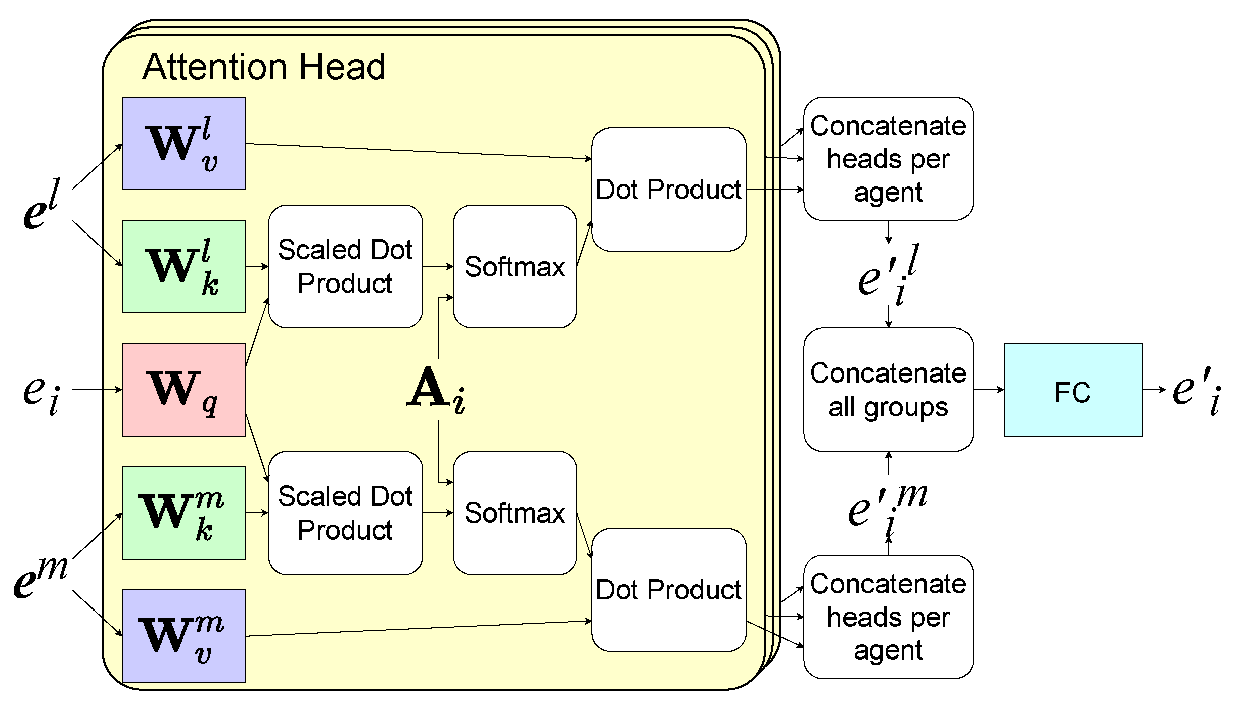
3.2. Hierarchical Graph Attention Network (HGAT)
4. System Model and Problem Statement
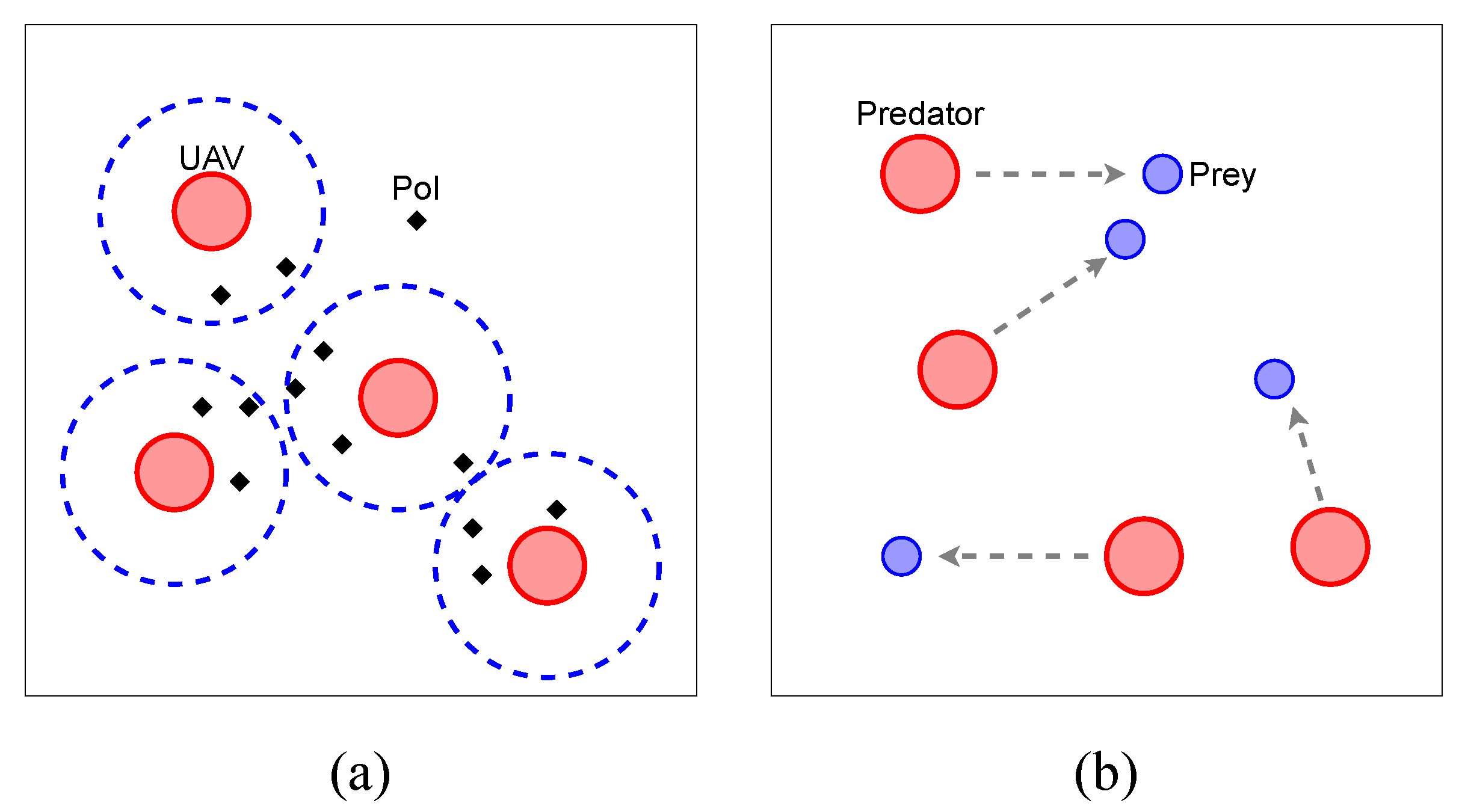
4.1. UAV Recon
4.2. Predator-Prey
5. HGAT-Based Multi-Agent Coordination Control Method
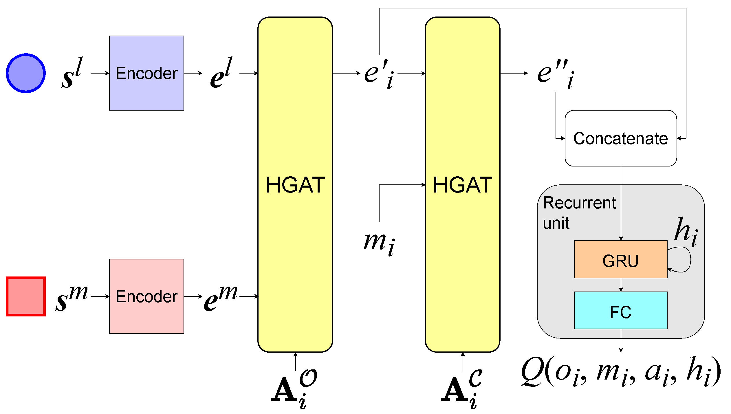
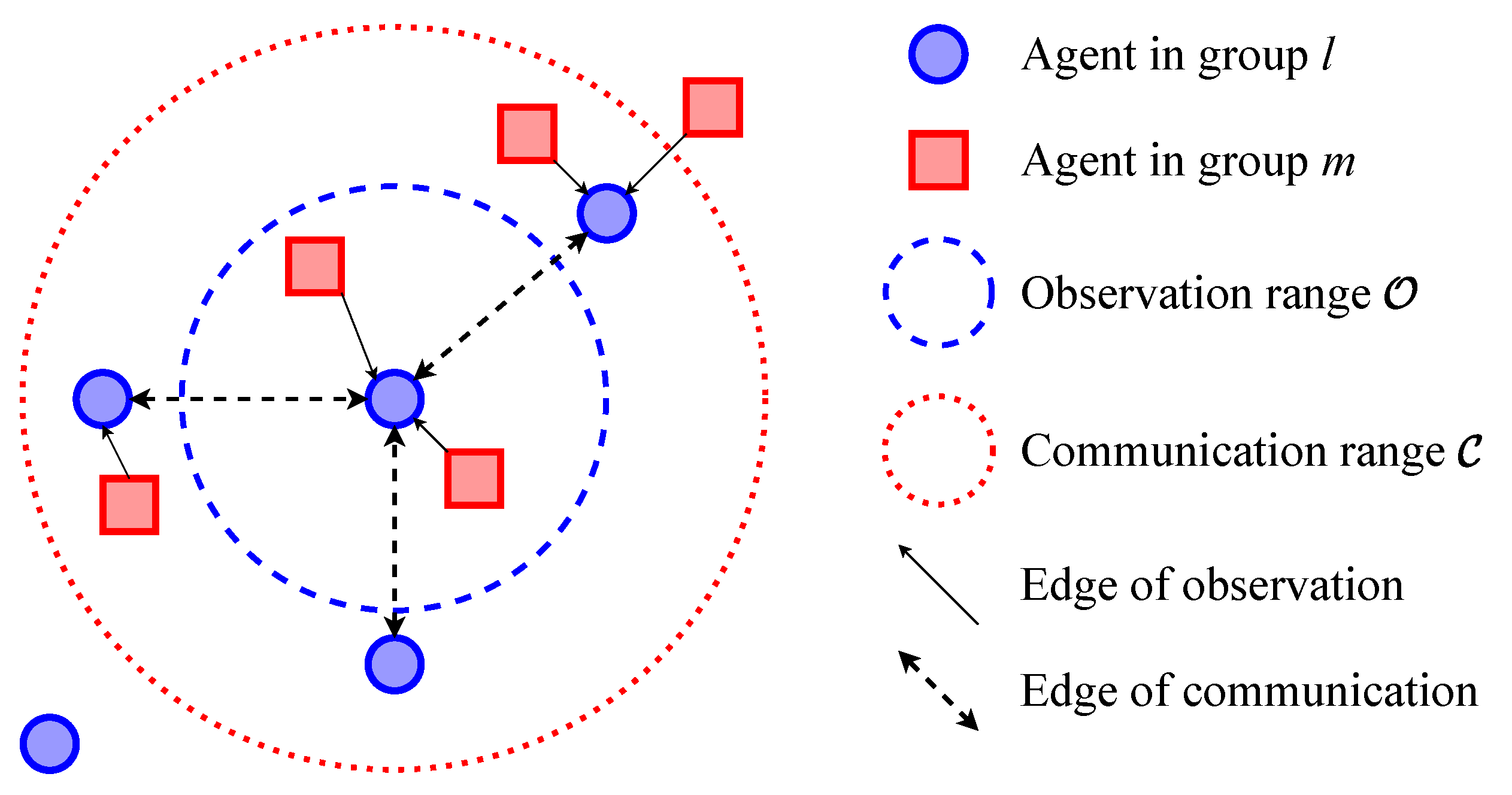
5.1. HGAT-Based Observation Aggregation and Inter-Agent Communication
5.2. Implementation in a Value-Based Framework
5.3. Implementation in an Actor–Critic Framework
6. Simulation
6.1. Set Up
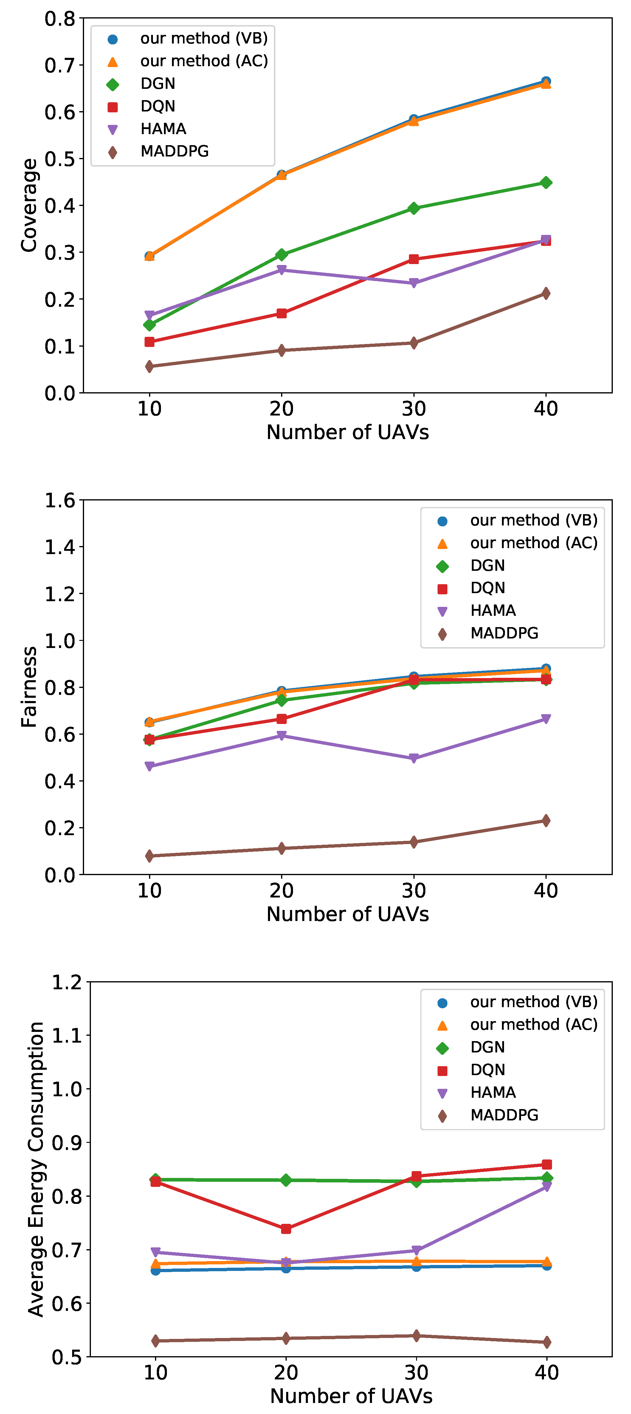
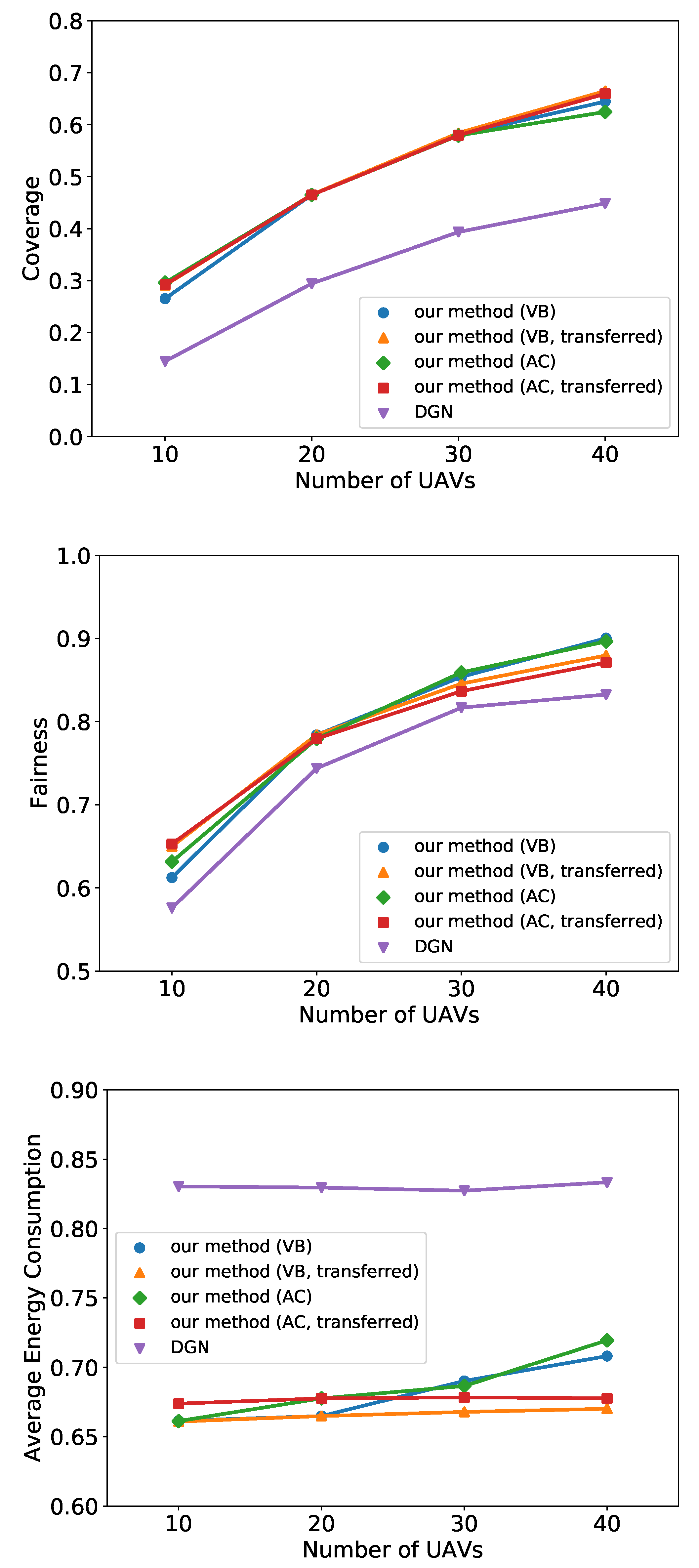
6.2. UAV Recon
6.3. Predator-Prey
7. Discussion
8. Conclusions
Author Contributions
Funding
Institutional Review Board Statement
Informed Consent Statement
Data Availability Statement
Conflicts of Interest
Abbreviations
| AC | Actor–Critic |
| ACO | Ant Colony Optimization |
| COMA | COunterfactual Multi-Agent |
| Dec-POMDP | Decentralized Partially Observable Markov Decision Process |
| DGN | Deep Graph Network |
| DNN | Deep Neural Network |
| DQN | Deep Q-Network |
| DRGN | Deep Recurrent Graph Network |
| DRL | Deep Reinforcement Learning |
| GA | Genetic Algorithm |
| GAT | Graph Attention neTwork |
| GCN | Graph Convolutional Network |
| GRU | Gated Recurrent Unit |
| HAMA | Hierarchical Graph Attention-Based Multi-Agent Actor–Critic |
| HGAT | Hierarchical Graph Attention neTwork |
| MAAC | Multi-Actor-Attention-Critic |
| MADDPG | Multi-Agent Deep Deterministic Policy Gradient |
| MARL | Multi-Agent Reinforcement Learning |
| PoI | Point-of-Interest |
| QoS | Quality of Service |
| RL | Reinforcement Learning |
| RSH | Randomized Search Heuristic |
| SARSA | State-Action-Reward-State-Action |
| TRPO | Trust Region Policy Optimization |
| UAV | Unmanned Aerial Vehicle |
| UAV-MBS | Unmanned Aerial Vehicle Mobile Base Station |
| VB | Value-Based |
Appendix A. Ablation Study
- Without H: removing the first HGAT layer;
- Without G: removing GRU in the recurrent unit;
- Without C: disabling inter-agent communication.

| Model | Metric | ||
|---|---|---|---|
| Coverage | Fairness | Energy Consumption | |
| Our method | 0.466 ± 0.046 | 0.784 ± 0.061 | 0.665 ± 0.015 |
| Without H | 0.103 ± 0.022 | 0.696 ± 0.087 | 0.710 ± 0.011 |
| Without G | 0.349 ± 0.065 | 0.726 ± 0.116 | 0.730 ± 0.017 |
| Without C | 0.412 ± 0.058 | 0.749 ± 0.081 | 0.668 ± 0.023 |
References
- Dorri, A.; Kanhere, S.S.; Jurdak, R. Multi-agent systems: A survey. IEEE Access 2018, 6, 28573–28593. [Google Scholar] [CrossRef]
- Gutierrez-Garcia, J.O.; Sim, K.M. Agent-based cloud bag-of-tasks execution. J. Syst. Softw. 2015, 104, 17–31. [Google Scholar] [CrossRef]
- Claes, R.; Holvoet, T.; Weyns, D. A decentralized approach for anticipatory vehicle routing using delegate multiagent systems. IEEE Trans. Intell. Transp. Syst. 2011, 12, 364–373. [Google Scholar] [CrossRef] [Green Version]
- Ota, J. Multi-agent robot systems as distributed autonomous systems. Adv. Eng. Inform. 2006, 20, 59–70. [Google Scholar] [CrossRef]
- Iñigo-Blasco, P.; Diaz-del Rio, F.; Romero-Ternero, M.C.; Cagigas-Muñiz, D.; Vicente-Diaz, S. Robotics software frameworks for multi-agent robotic systems development. Robot. Auton. Syst. 2012, 60, 803–821. [Google Scholar] [CrossRef]
- Liu, C.H.; Chen, Z.; Tang, J.; Xu, J.; Piao, C. Energy-efficient UAV control for effective and fair communication coverage: A deep reinforcement learning approach. IEEE J. Sel. Areas Commun. 2018, 36, 2059–2070. [Google Scholar] [CrossRef]
- Zhang, Y.; Mou, Z.; Gao, F.; Jiang, J.; Ding, R.; Han, Z. UAV-enabled secure communications by multi-agent deep reinforcement learning. IEEE Trans. Veh. Technol. 2020, 69, 11599–11611. [Google Scholar] [CrossRef]
- Ryu, H.; Shin, H.; Park, J. Multi-agent actor-critic with hierarchical graph attention network. In Proceedings of the AAAI Conference on Artificial Intelligence, New York, NY, USA, 7–12 February 2020; Volume 34, pp. 7236–7243. [Google Scholar] [CrossRef]
- Cho, K.; Van Merriënboer, B.; Bahdanau, D.; Bengio, Y. On the properties of neural machine translation: Encoder-decoder approaches. arXiv 2014, arXiv:1409.1259. [Google Scholar]
- Ramirez-Atencia, C.; Bello-Orgaz, G.; R-Moreno, M.D.; Camacho, D. Solving complex multi-UAV mission planning problems using multi-objective genetic algorithms. Soft Comput. 2017, 21, 4883–4900. [Google Scholar] [CrossRef]
- Zhen, Z.; Xing, D.; Gao, C. Cooperative search-attack mission planning for multi-UAV based on intelligent self-organized algorithm. Aerosp. Sci. Technol. 2018, 76, 402–411. [Google Scholar] [CrossRef]
- Altshuler, Y.; Wagner, I.; Yanovski, V.; Bruckstein, A. Multi-agent Cooperative Cleaning of Expanding Domains. Int. J. Robot. Res. 2010, 30, 1037–1071. [Google Scholar] [CrossRef]
- Altshuler, Y.; Pentland, A.; Bruckstein, A.M. Swarms and Network Intelligence in Search; Springer: Berlin/Heidelberg, Germany, 2018. [Google Scholar]
- Altshuler, Y.; Bruckstein, A.M. Static and expanding grid coverage with ant robots: Complexity results. Theor. Comput. Sci. 2011, 412, 4661–4674. [Google Scholar] [CrossRef] [Green Version]
- Cho, S.W.; Park, H.J.; Lee, H.; Shim, D.H.; Kim, S.Y. Coverage path planning for multiple unmanned aerial vehicles in maritime search and rescue operations. Comput. Ind. Eng. 2021, 161, 107612. [Google Scholar] [CrossRef]
- Apostolopoulos, P.A.; Torres, M.; Tsiropoulou, E.E. Satisfaction-aware data offloading in surveillance systems. In Proceedings of the 14th Workshop on Challenged Networks, Los Cabos, Mexico, 25 October 2019; pp. 21–26. [Google Scholar] [CrossRef]
- Rummery, G.A.; Niranjan, M. On-Line Q-Learning Using Connectionist Systems; Citeseer: University Park, PA, USA, 1994; Volume 37. [Google Scholar]
- Shamsoshoara, A.; Khaledi, M.; Afghah, F.; Razi, A.; Ashdown, J. Distributed cooperative spectrum sharing in uav networks using multi-agent reinforcement learning. In Proceedings of the 2019 16th IEEE Annual Consumer Communications & Networking Conference (CCNC), Las Vegas, NV, USA, 11–14 January 2019; pp. 1–6. [Google Scholar] [CrossRef] [Green Version]
- Watkins, C.J.; Dayan, P. Q-learning. Mach. Learn. 1992, 8, 279–292. [Google Scholar] [CrossRef]
- Pinto, L.; Davidson, J.; Sukthankar, R.; Gupta, A. Robust adversarial reinforcement learning. In Proceedings of the International Conference on Machine Learning, Sydney, NSW, Australia, 6–11 August 2017; pp. 2817–2826. [Google Scholar]
- Finn, C.; Yu, T.; Fu, J.; Abbeel, P.; Levine, S. Generalizing skills with semi-supervised reinforcement learning. arXiv 2016, arXiv:1612.00429. [Google Scholar]
- Lowe, R.; WU, Y.; Tamar, A.; Harb, J.; Pieter Abbeel, O.; Mordatch, I. Multi-Agent Actor-Critic for Mixed Cooperative-Competitive Environments. In Advances in Neural Information Processing Systems 30; Guyon, I., Luxburg, U.V., Bengio, S., Wallach, H., Fergus, R., Vishwanathan, S., Garnett, R., Eds.; Curran Associates, Inc.: Red Hook, NY, USA, 2017; pp. 6379–6390. [Google Scholar]
- Foerster, J.N.; Farquhar, G.; Afouras, T.; Nardelli, N.; Whiteson, S. Counterfactual multi-agent policy gradients. In Proceedings of the Thirty-Second AAAI Conference on Artificial Intelligence, New Orleans, LA, USA, 2–7 February 2018. [Google Scholar]
- Tan, M. Multi-agent reinforcement learning: Independent vs. cooperative agents. In Proceedings of the Tenth International Conference on Machine Learning, Long Beach, CA, USA, 9–15 June 1993; pp. 330–337. [Google Scholar]
- Iqbal, S.; Sha, F. Actor-Attention-Critic for Multi-Agent Reinforcement Learning. In Proceedings of the 36th International Conference on Machine Learning, Long Beach, CA, USA, 9–15 June 2019; Chaudhuri, K., Salakhutdinov, R., Eds.; PMLR: Long Beach, CA, USA, 2019; Volume 97, pp. 2961–2970. [Google Scholar]
- Jiang, J.; Dun, C.; Huang, T.; Lu, Z. Graph convolutional reinforcement learning. arXiv 2018, arXiv:1810.09202. [Google Scholar]
- Liu, C.H.; Ma, X.; Gao, X.; Tang, J. Distributed energy-efficient multi-UAV navigation for long-term communication coverage by deep reinforcement learning. IEEE Trans. Mob. Comput. 2019, 19, 1274–1285. [Google Scholar] [CrossRef]
- Khan, A.; Tolstaya, E.; Ribeiro, A.; Kumar, V. Graph policy gradients for large scale robot control. In Proceedings of the Conference on Robot Learning, Cambridge, MA, USA, 16–18 November 2020; pp. 823–834. [Google Scholar]
- Walker, O.; Vanegas, F.; Gonzalez, F.; Koenig, S. A deep reinforcement learning framework for UAV navigation in indoor environments. In Proceedings of the 2019 IEEE Aerospace Conference, Big Sky, MT, USA, 2–9 March 2019; pp. 1–14. [Google Scholar]
- Schulman, J.; Levine, S.; Abbeel, P.; Jordan, M.; Moritz, P. Trust region policy optimization. In Proceedings of the International Conference on Machine Learning, Lille, France, 7–9 July 2015; pp. 1889–1897. [Google Scholar]
- Ye, Z.; Wang, K.; Chen, Y.; Jiang, X.; Song, G. Multi-UAV Navigation for Partially Observable Communication Coverage by Graph Reinforcement Learning. IEEE Trans. Mob. Comput. 2022. [Google Scholar] [CrossRef]
- Veličković, P.; Cucurull, G.; Casanova, A.; Romero, A.; Lio, P.; Bengio, Y. Graph attention networks. arXiv 2017, arXiv:1710.10903. [Google Scholar]
- Bernstein, D.S.; Givan, R.; Immerman, N.; Zilberstein, S. The complexity of decentralized control of Markov decision processes. Math. Oper. Res. 2002, 27, 819–840. [Google Scholar] [CrossRef]
- Sutton, R.S.; McAllester, D.A.; Singh, S.P.; Mansour, Y. Policy gradient methods for reinforcement learning with function approximation. In Advances in Neural Information Processing Systems; MIT Press: Cambridge, MA, USA, 2000; pp. 1057–1063. [Google Scholar]
- Mnih, V.; Kavukcuoglu, K.; Silver, D.; Rusu, A.A.; Veness, J.; Bellemare, M.G.; Graves, A.; Riedmiller, M.; Fidjeland, A.K.; Ostrovski, G.; et al. Human-level control through deep reinforcement learning. Nature 2015, 518, 529. [Google Scholar] [CrossRef] [PubMed]
- Williams, R.J. Simple statistical gradient-following algorithms for connectionist reinforcement learning. Mach. Learn. 1992, 8, 229–256. [Google Scholar] [CrossRef] [Green Version]
- Konda, V.R.; Tsitsiklis, J.N. Actor-critic algorithms. In Advances in Neural Information Processing Systems; MIT Press: Cambridge, MA, USA, 2000; pp. 1008–1014. [Google Scholar]
- Jain, R.K.; Chiu, D.M.W.; Hawe, W.R. A Quantitative Measure of Fairness and Discrimination; Eastern Research Laboratory, Digital Equipment Corporation: Hudson, MA, USA, 1984. [Google Scholar]
- Weaver, L.; Tao, N. The optimal reward baseline for gradient-based reinforcement learning. arXiv 2013, arXiv:1301.2315. [Google Scholar]
- Heess, N.; Hunt, J.J.; Lillicrap, T.P.; Silver, D. Memory-based control with recurrent neural networks. arXiv 2015, arXiv:1512.04455. [Google Scholar]
- Nair, V.; Hinton, G.E. Rectified Linear Units Improve Restricted Boltzmann Machines. In Proceedings of the 27th International Conference on Machine Learning (ICML 2010), Haifa, Israel, 21–24 June 2010; pp. 807–814. [Google Scholar]
- Jang, E.; Gu, S.; Poole, B. Categorical reparameterization with gumbel-softmax. arXiv 2016, arXiv:1611.01144. [Google Scholar]


| Parameters | Settings |
|---|---|
| Target Area | 200 × 200 |
| Number of PoIs | 120 |
| Recon Range | 10 |
| Observation Range | 15 |
| Communication Range | 30 |
| Maximum Speed | 10/s |
| Energy Consumption for Hovering | 0.5 |
| Energy Consumption for Movement | 0.5 |
| Penalty Factor p | 1 |
| Importance Factor | 1 |
| Importance Factor | 0.1 |
| Timeslots of Each Episode | 100 |
| Parameters | Settings |
|---|---|
| Target Area | 100 × 100 |
| Number of Predators | 5 |
| Number of Preys | 5 |
| Attack Range | 8 |
| Observation Range | 30 |
| Communication Range | 100 |
| Maximum Speed of Predators | 10/s |
| Maximum Speed of Preys | 12/s |
| Timeslots of Each Episode | 100 |
| Predator | Prey | ||
|---|---|---|---|
| Our Method | DGN | DQN | |
| Our method | 0.331± 0.088 | 0.535± 0.086 | 0.591± 0.101 |
| DGN | 0.051 ± 0.060 | 0.271 ± 0.095 | 0.386 ± 0.095 |
| DQN | 0.014 ± 0.034 | 0.173 ± 0.086 | 0.120 ± 0.078 |
| Predator | Prey | ||
| Our Method | HAMA | MADDPG | |
| Our method | 0.331± 0.088 | 0.787± 0.027 | 0.472± 0.098 |
| HAMA | 0.051 ± 0.050 | 0.351 ± 0.050 | 0.403 ± 0.091 |
| MADDPG | 0.038 ± 0.048 | 0.239 ± 0.090 | 0.051 ± 0.057 |
Publisher’s Note: MDPI stays neutral with regard to jurisdictional claims in published maps and institutional affiliations. |
© 2022 by the authors. Licensee MDPI, Basel, Switzerland. This article is an open access article distributed under the terms and conditions of the Creative Commons Attribution (CC BY) license (https://creativecommons.org/licenses/by/4.0/).
Share and Cite
Chen, Y.; Song, G.; Ye, Z.; Jiang, X. Scalable and Transferable Reinforcement Learning for Multi-Agent Mixed Cooperative–Competitive Environments Based on Hierarchical Graph Attention. Entropy 2022, 24, 563. https://doi.org/10.3390/e24040563
Chen Y, Song G, Ye Z, Jiang X. Scalable and Transferable Reinforcement Learning for Multi-Agent Mixed Cooperative–Competitive Environments Based on Hierarchical Graph Attention. Entropy. 2022; 24(4):563. https://doi.org/10.3390/e24040563
Chicago/Turabian StyleChen, Yining, Guanghua Song, Zhenhui Ye, and Xiaohong Jiang. 2022. "Scalable and Transferable Reinforcement Learning for Multi-Agent Mixed Cooperative–Competitive Environments Based on Hierarchical Graph Attention" Entropy 24, no. 4: 563. https://doi.org/10.3390/e24040563
APA StyleChen, Y., Song, G., Ye, Z., & Jiang, X. (2022). Scalable and Transferable Reinforcement Learning for Multi-Agent Mixed Cooperative–Competitive Environments Based on Hierarchical Graph Attention. Entropy, 24(4), 563. https://doi.org/10.3390/e24040563