
Bayesian and E-Bayesian Estimations of Bathtub-Shaped Distribution under Generalized Type-I Hybrid Censoring


Abstract
:1. Introduction
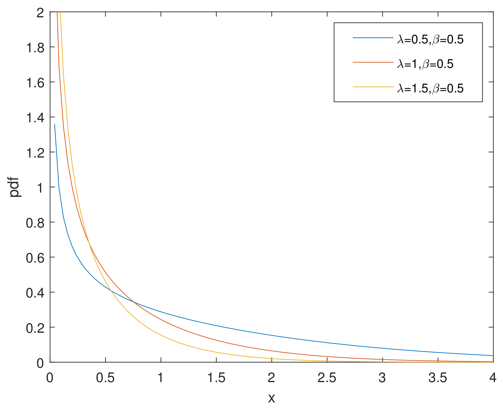
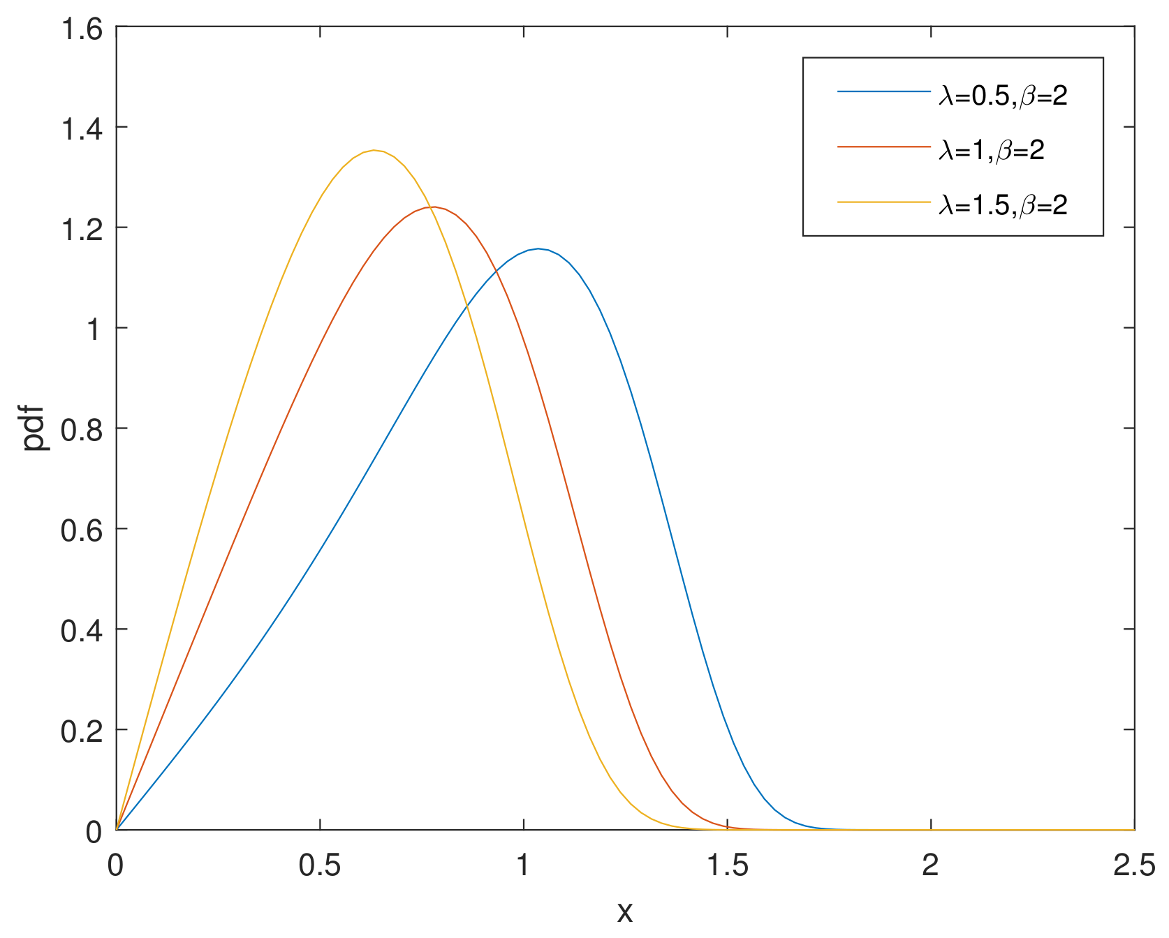
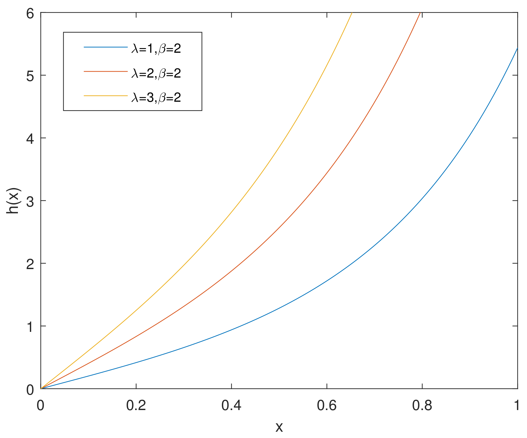
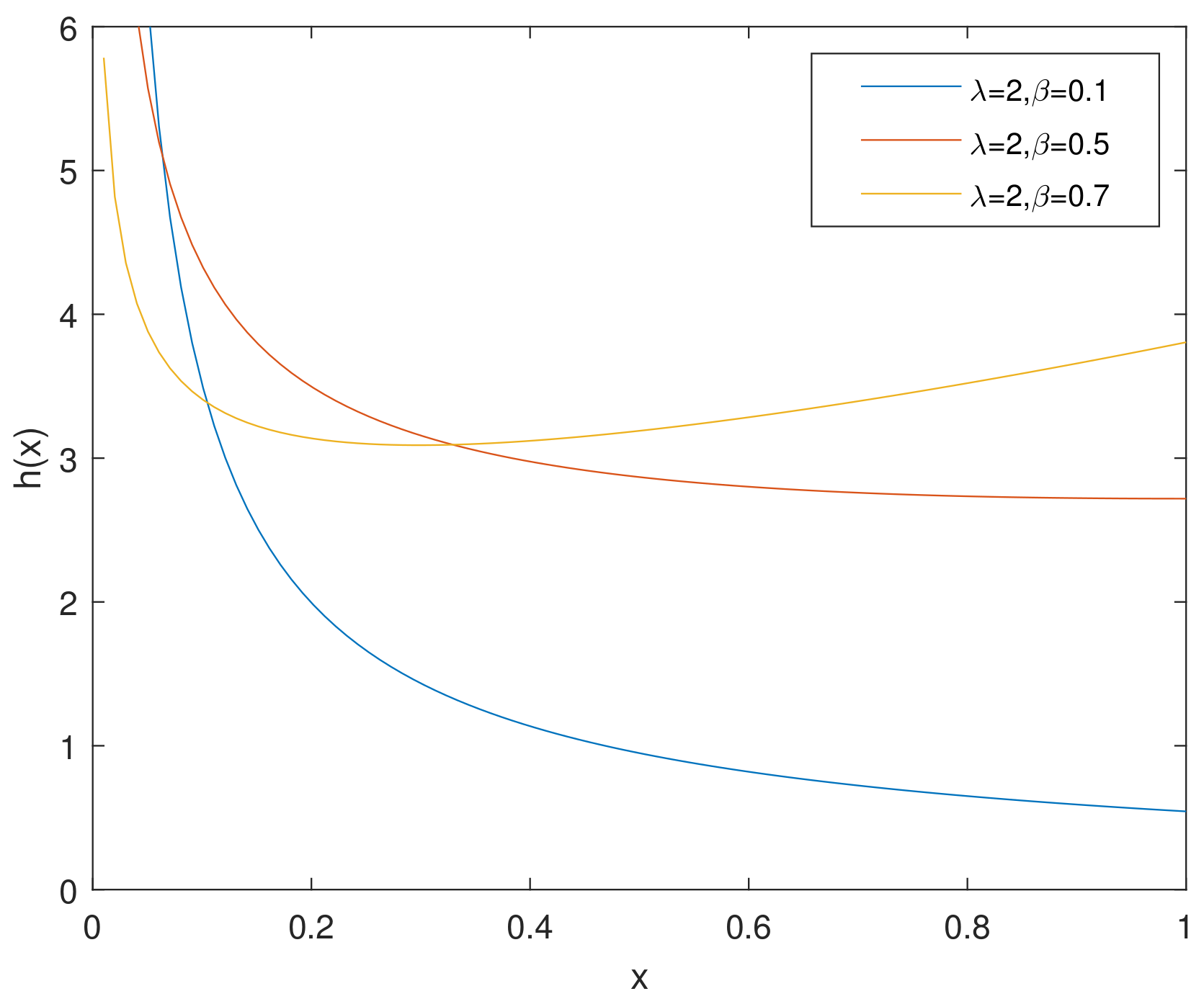
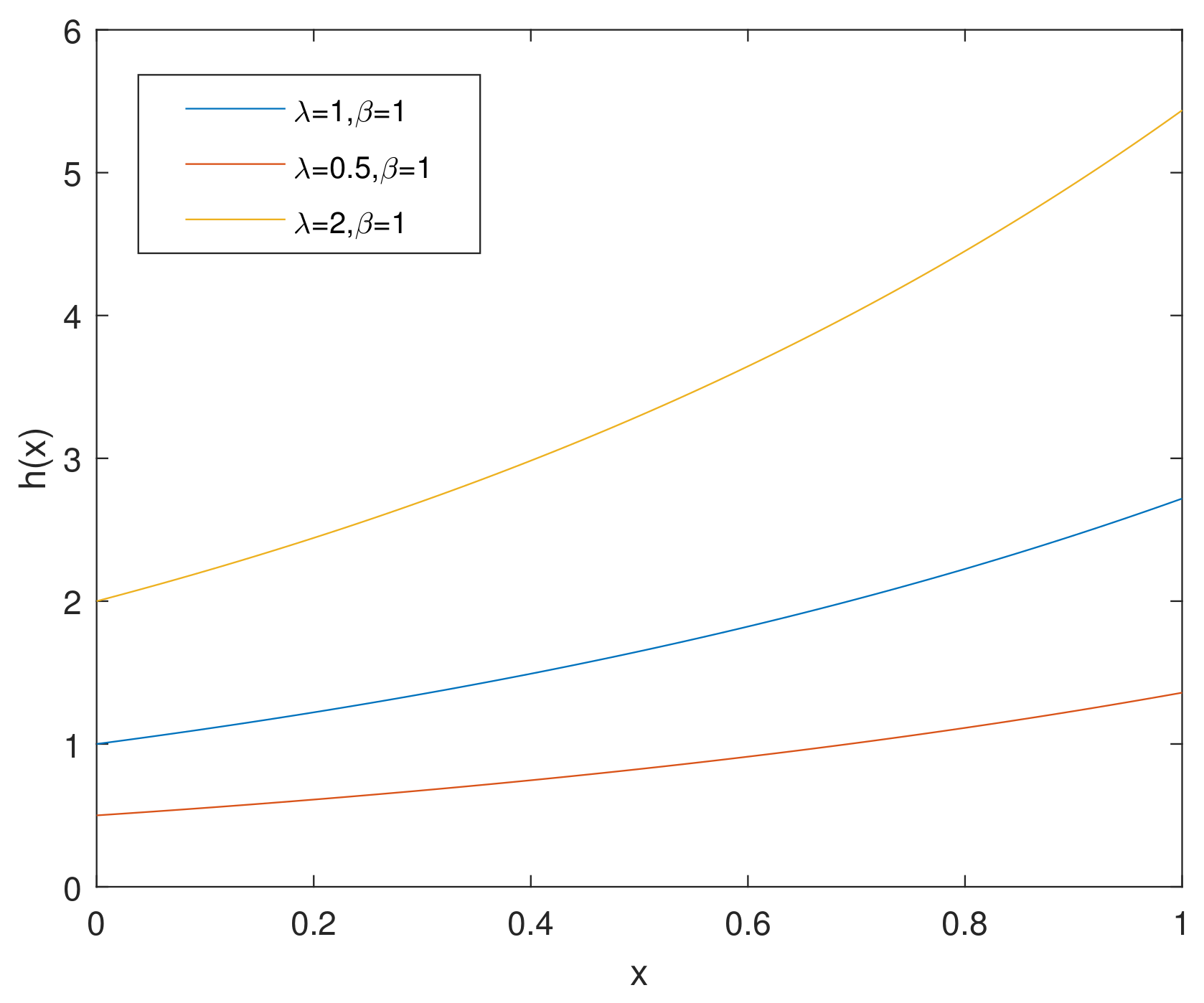
1.1. Bathtub-Shaped Distribution
1.2. Generalized Hybrid Type-I Censoring Scheme
- Type-I censoring: terminate at T.
- Hybrid Type-I censoring: terminate at .
- Type-I GHCS: terminate at where and k is the minimum acceptable number of failures fixed before the experiment.
- Case I: , when .
- Case II: , when .
- Case III: , when .
2. Bayesian Estimation
3. E-Bayesian Estimation
3.1. E-Bayesian Estimations Based on SE Loss Function
3.2. E-Bayesian Estimations Based on a LINEX Loss Function
3.3. E-Bayesian Estimations of
4. Estimation with Two Unknown Parameters
4.1. Bayesian Estimation
4.2. E-Bayesian Estimation
5. MCMC Method and Simulation Study
| Algorithm 1 MCMC algorithm. |
|
| Algorithm 2 The algorithm of generating and analyzing data. |
|
- 1.
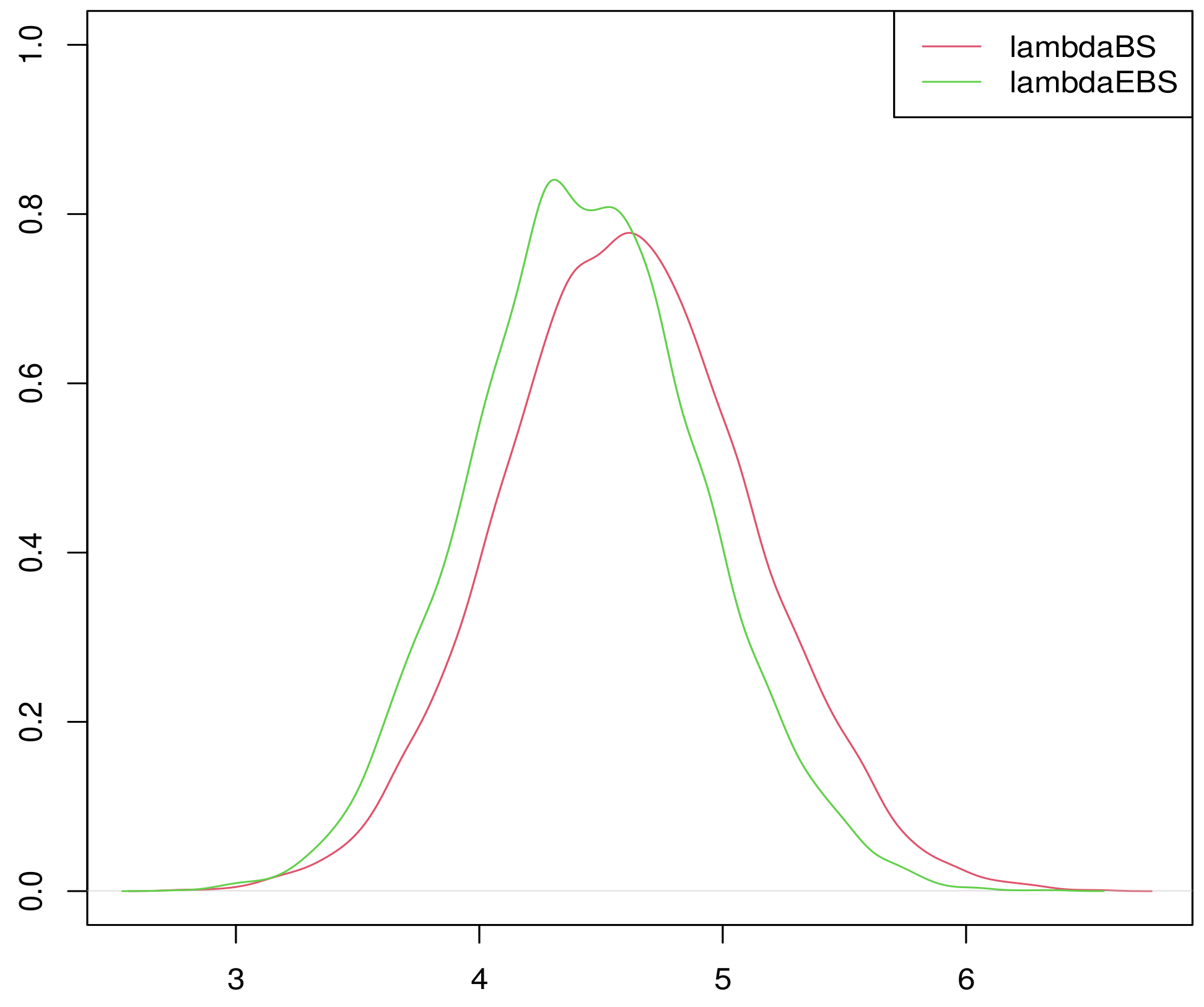
- Both estimates are close to their theoretical values under different methods and loss functions.
- 2.
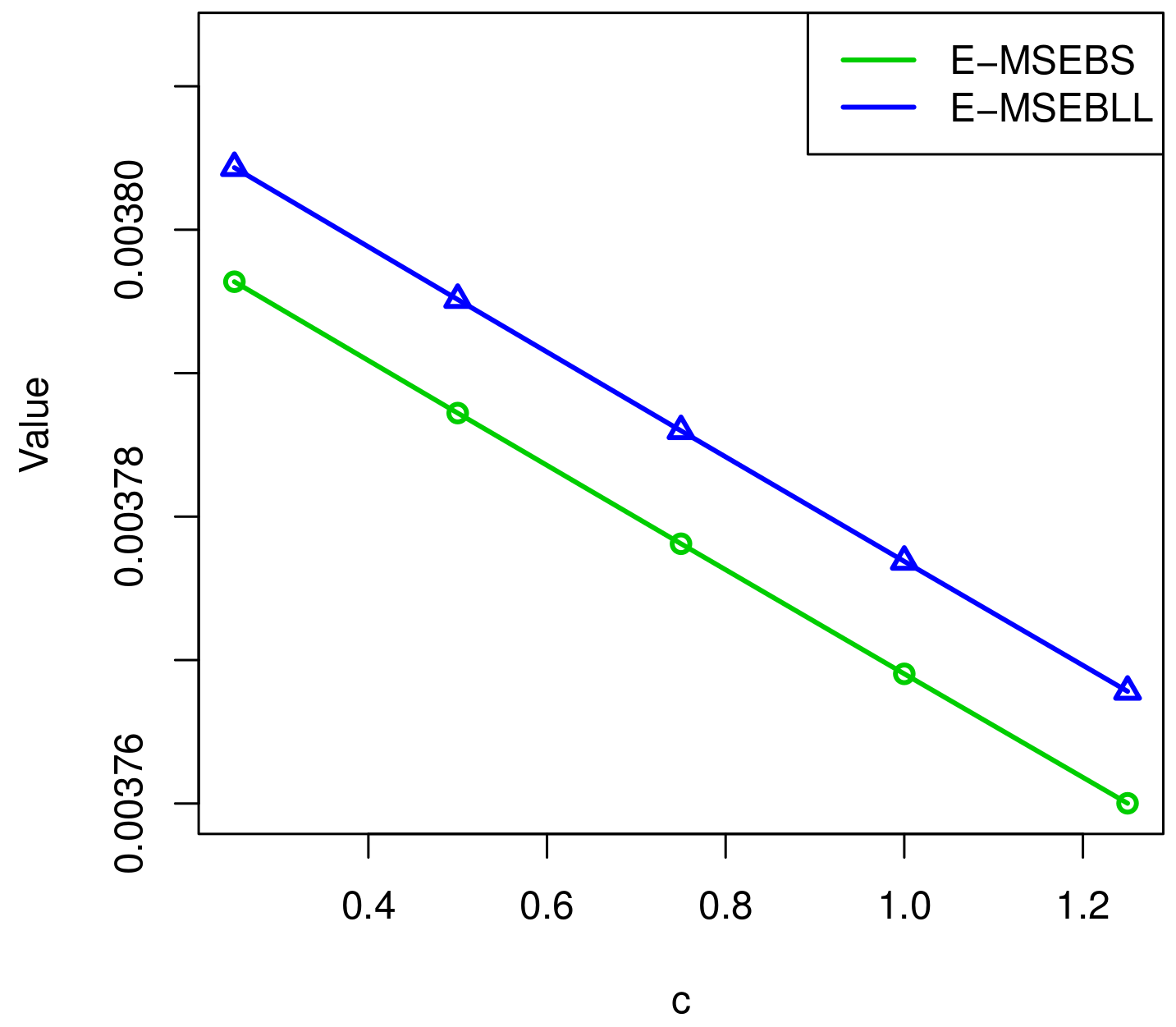
- The mean square errors of the E-Bayesian estimations of parameter and are smaller than those of the Bayesian estimations. Therefore, the efficiency of the E-Bayesian method is higher in the sense of a smaller .
- 3.
- The of estimations under an SE loss function are less than those based on a LINEX loss function. Thus, the SE loss function is more efficient to generate estimates.
- 4.
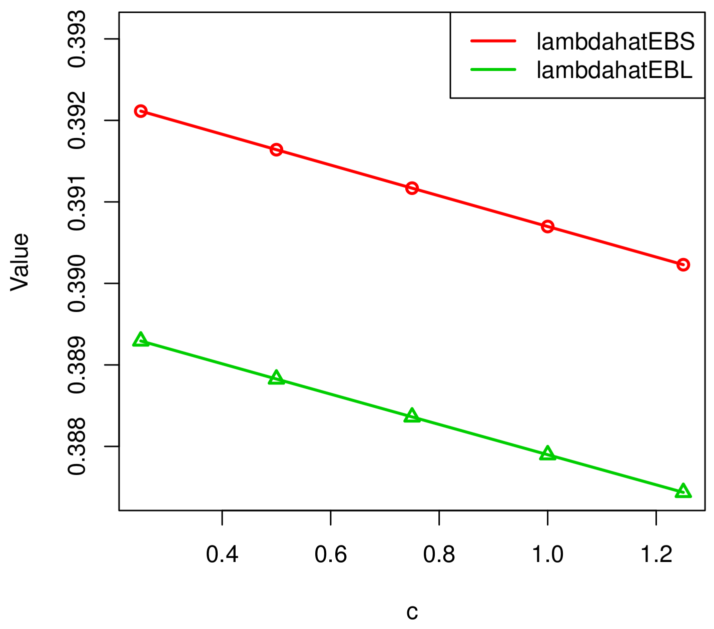
- As increases, the of the estimate decreases, and the average interval length of reduces. To conclude, the performance of estimates will improve with the size of the sample increases.
6. Illustrative Example
7. Conclusions
Author Contributions
Funding
Data Availability Statement
Conflicts of Interest
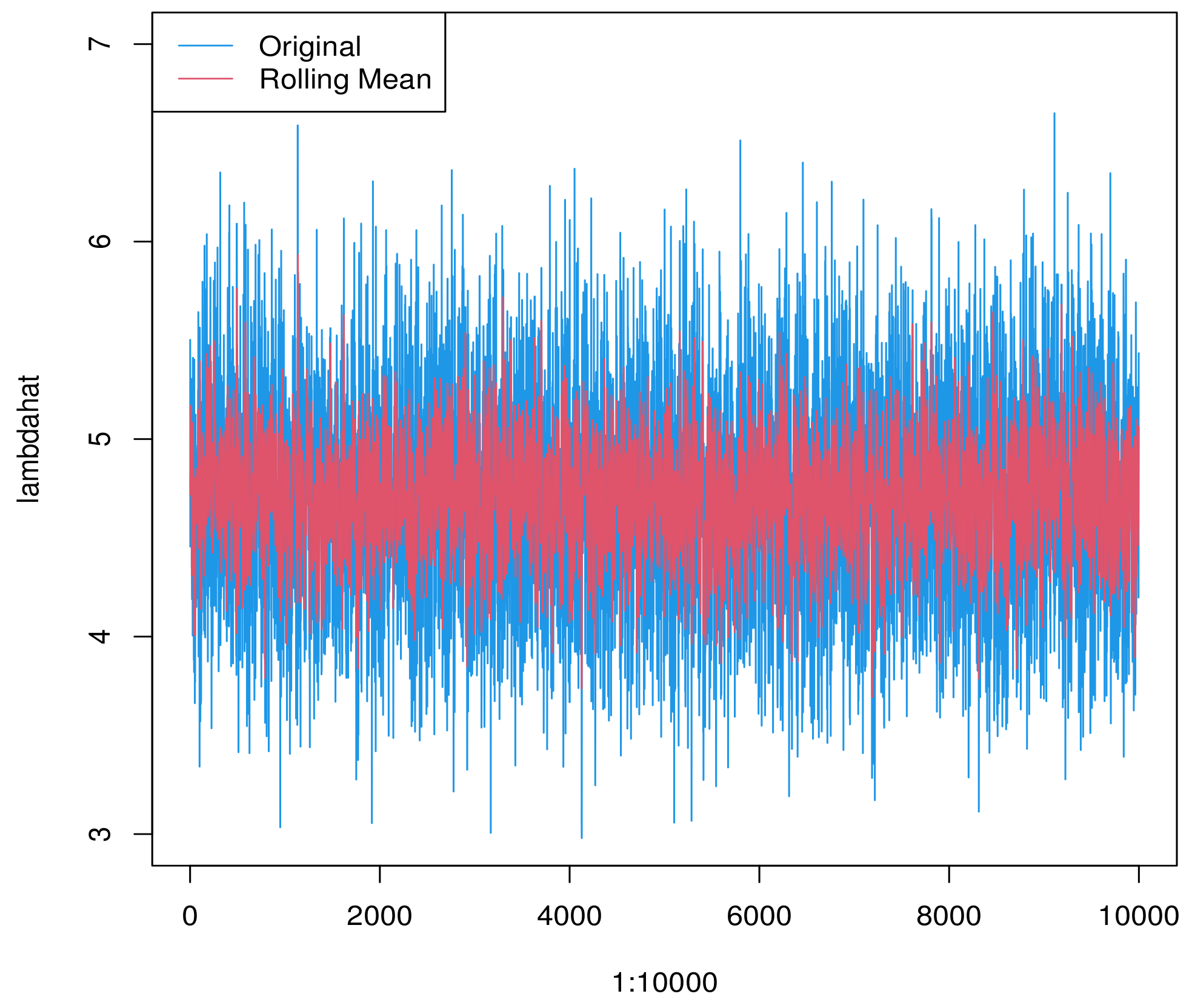
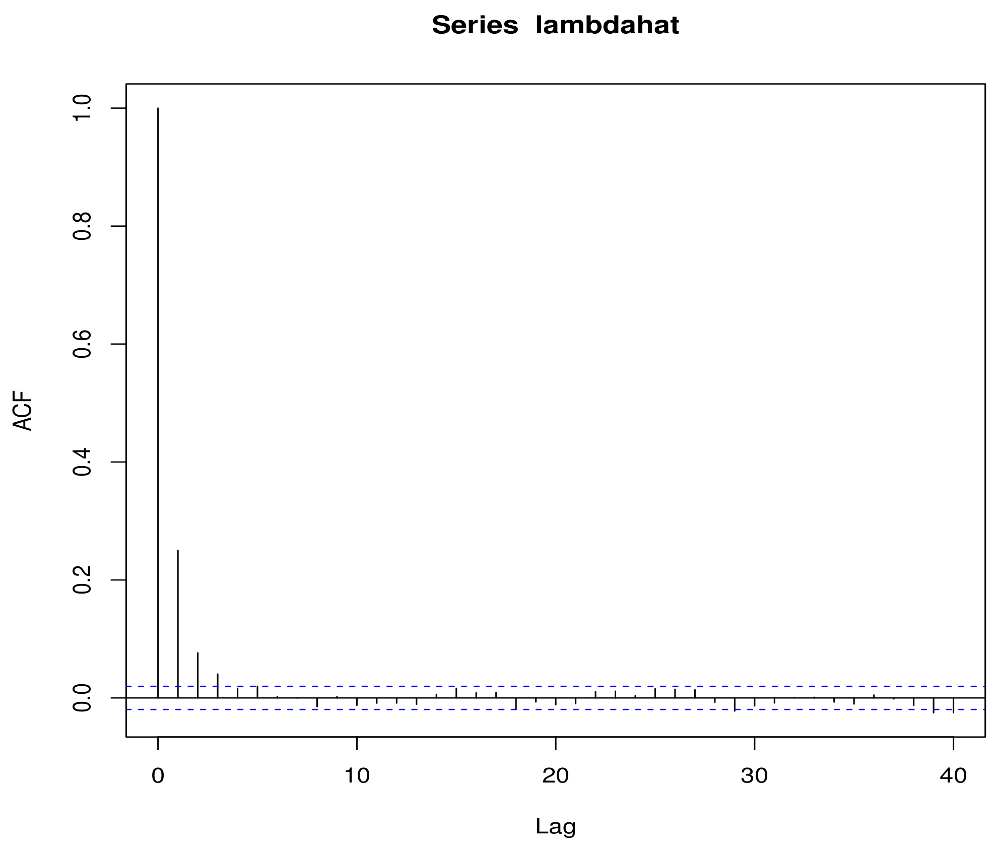
Appendix A. MCMC Outputs


Appendix B. The Robustness of the Simulation with Different h

| n | T | c | |||||||||
|---|---|---|---|---|---|---|---|---|---|---|---|
| 50 | (40,30) | 0.2 | 0.5 | 2.6054 | 0.2292 | 2.5742 | 0.2245 | 2.3134 | 0.3251 | 2.2878 | 0.3166 |
| 0.4 | 2.5541 | 0.1832 | 2.5287 | 0.1801 | 2.3135 | 0.2450 | 2.2920 | 0.2399 | |||
| 80 | (60,40) | 0.2 | 2.5796 | 0.1665 | 2.5567 | 0.1640 | 2.3585 | 0.2193 | 2.3387 | 0.2152 | |
| 0.4 | 2.5377 | 0.1142 | 2.5217 | 0.1130 | 2.3804 | 0.1402 | 2.3661 | 0.1384 | |||
| 120 | (90,60) | 0.2 | 2.5481 | 0.1085 | 2.5329 | 0.1074 | 2.3981 | 0.1324 | 2.3844 | 0.1308 | |
| 0.4 | 2.5221 | 0.0751 | 2.5115 | 0.0745 | 2.4158 | 0.0867 | 2.4060 | 0.0860 | |||
| 50 | (40,30) | 0.2 | 1 | 2.6092 | 0.2299 | 2.5779 | 0.2251 | 2.3164 | 0.3262 | 2.2908 | 0.3177 |
| 0.4 | 2.5552 | 0.1833 | 2.5298 | 0.1802 | 2.3145 | 0.2451 | 2.2930 | 0.2401 | |||
| 80 | (60,40) | 0.2 | 2.5645 | 0.1646 | 2.5418 | 0.1621 | 2.3457 | 0.2163 | 2.3261 | 0.2123 | |
| 0.4 | 2.5385 | 0.1143 | 2.5226 | 0.1131 | 2.3812 | 0.1403 | 2.3668 | 0.1385 | |||
| 120 | (90,60) | 0.2 | 2.5523 | 0.1089 | 2.5371 | 0.1078 | 2.4018 | 0.1329 | 2.3881 | 0.1313 | |
| 0.4 | 2.5243 | 0.0752 | 2.5137 | 0.0747 | 2.4179 | 0.0869 | 2.4080 | 0.0862 | |||
| 50 | (40,30) | 0.2 | 1.5 | 2.6017 | 0.2285 | 2.5706 | 0.2238 | 2.3105 | 0.3237 | 2.2850 | 0.3153 |
| 0.4 | 2.5570 | 0.1835 | 2.5316 | 0.1805 | 2.3161 | 0.2456 | 2.2945 | 0.2406 | |||
| 80 | (60,40) | 0.2 | 2.5778 | 0.1663 | 2.5548 | 0.1638 | 2.3569 | 0.2190 | 2.3372 | 0.2150 | |
| 0.4 | 2.5392 | 0.1144 | 2.5233 | 0.1132 | 2.3818 | 0.1404 | 2.3675 | 0.1386 | |||
| 120 | (90,60) | 0.2 | 2.5416 | 0.1080 | 2.5266 | 0.1069 | 2.3924 | 0.1316 | 2.3788 | 0.1300 | |
| 0.4 | 2.5258 | 0.0752 | 2.5153 | 0.0747 | 2.4193 | 0.0869 | 2.4095 | 0.0863 |
| n | T | c | |||||||||
|---|---|---|---|---|---|---|---|---|---|---|---|
| 50 | (40,30) | 0.2 | 0.5 | 2.6014 | 0.2285 | 2.5703 | 0.2238 | 2.5460 | 0.2320 | 2.5160 | 0.2272 |
| 0.4 | 2.5572 | 0.1835 | 2.5318 | 0.1804 | 2.5124 | 0.1857 | 2.4877 | 0.1825 | |||
| 80 | (60,40) | 0.2 | 2.5721 | 0.1656 | 2.5493 | 0.1631 | 2.5316 | 0.1674 | 2.5094 | 0.1648 | |
| 0.4 | 2.5373 | 0.1142 | 2.5213 | 0.1130 | 2.5092 | 0.1150 | 2.4935 | 0.1138 | |||
| 120 | (90,60) | 0.2 | 2.5559 | 0.1092 | 2.5407 | 0.1081 | 2.5290 | 0.1100 | 2.5140 | 0.1088 | |
| 0.4 | 2.5281 | 0.0754 | 2.5175 | 0.0748 | 2.5095 | 0.0757 | 2.4990 | 0.0752 | |||
| 50 | (40,30) | 0.2 | 1 | 2.6168 | 0.2312 | 2.5854 | 0.2265 | 2.5607 | 0.2348 | 2.5304 | 0.2299 |
| 0.4 | 2.5595 | 0.1837 | 2.5341 | 0.1806 | 2.5146 | 0.1859 | 2.4900 | 0.1827 | |||
| 80 | (60,40) | 0.2 | 2.5747 | 0.1659 | 2.5519 | 0.1634 | 2.5342 | 0.1677 | 2.5119 | 0.1651 | |
| 0.4 | 2.5361 | 0.1141 | 2.5201 | 0.1129 | 2.5079 | 0.1150 | 2.4923 | 0.1137 | |||
| 120 | (90,60) | 0.2 | 2.5527 | 0.1089 | 2.5376 | 0.1078 | 2.5259 | 0.1097 | 2.5110 | 0.1086 | |
| 0.4 | 2.5216 | 0.0750 | 2.5111 | 0.0745 | 2.5030 | 0.0754 | 2.4926 | 0.0748 | |||
| 50 | (40,30) | 0.2 | 1.5 | 2.6069 | 0.2297 | 2.5757 | 0.2249 | 2.5512 | 0.2332 | 2.5211 | 0.2283 |
| 0.4 | 2.5543 | 0.1831 | 2.5290 | 0.1801 | 2.5096 | 0.1853 | 2.4850 | 0.1821 | |||
| 80 | (60,40) | 0.2 | 2.5765 | 0.1661 | 2.5536 | 0.1636 | 2.5359 | 0.1679 | 2.5136 | 0.1653 | |
| 0.4 | 2.5309 | 0.1138 | 2.5149 | 0.1126 | 2.5028 | 0.1146 | 2.4872 | 0.1134 | |||
| 120 | (90,60) | 0.2 | 2.5459 | 0.1084 | 2.5308 | 0.1073 | 2.5192 | 0.1091 | 2.5044 | 0.1080 | |
| 0.4 | 2.5283 | 0.0754 | 2.5177 | 0.0749 | 2.5096 | 0.0757 | 2.4991 | 0.0752 |
Appendix C. MCMC Method for Two Unknown Parameters
| Algorithm A1 The MCMC algorithm for two unknown parameters. |
|
References
- Chen, Z. A new two-parameter lifetime distribution with bathtub shape or increasing failure rate function. Stat. Probab. Lett. 2008, 49, 155–161. [Google Scholar] [CrossRef]
- Hjorth, U. A reliability distribution with increasing, decreasing, and bathtub-shaped failure rate data. Technometrics 1980, 22, 99–107. [Google Scholar] [CrossRef]
- Mudholkar, G.S.; Srivastava, D.K. Exponentiated Weibull family for analyzing bathtub failure-rate data. IEEE Trans. Reliab. 1993, 42, 299–302. [Google Scholar] [CrossRef]
- Sarhan, A.M.; Hamilton, D.C.; Smith, B. Parameter estimation for a two-parameter bathtub-shaped lifetime distribution. Appl. Math. Model. 2012, 36, 5380–5392. [Google Scholar] [CrossRef]
- Wu, S. Estimation of the two-parameter bathtub-shaped lifetime distribution with progressive censoring. J. Appl. Stat. 2008, 35, 1139–1150. [Google Scholar] [CrossRef]
- Rastogi, M.K.; Tripathi, Y.M. Estimation using hybrid censored data from a two-parameter distribution with bathtub shape. Comput. Stat. Data Anal. 2013, 67, 268–281. [Google Scholar] [CrossRef]
- Smith, R.M.; Bain, L.J. An Exponential Power Life-Testing Distribution. Commun. Stat. Theory Methods 1975, 4, 469–481. [Google Scholar]
- Epstein, B. Truncated Life Tests in the Exponential Case. Ann. Math. Stat. 1954, 25, 555–564. [Google Scholar] [CrossRef]
- Chandrasekar, B.; Childs, A.; Balakrishnan, N. Exact Likelihood Inference for the Exponential Distribution under Generalized Type-I and Type-II Hybrid Censoring. Nav. Res. Logist. 2004, 51, 994–1004. [Google Scholar] [CrossRef]
- Balakrishnan, N.; Kundu, D. Hybrid censoring: Models, inferential results and applications. Comput. Stat. Data Anal. 2013, 57, 166–209. [Google Scholar] [CrossRef]
- Rabie, A.; Li, J. E-Bayesian Estimation for Burr-X Distribution Based on Generalized Type-I Hybrid Censoring Scheme. Am. J. Math. Manag. Sci. 2018, 41–55. [Google Scholar] [CrossRef] [Green Version]
- Sen, T.; Bhattacharya, R.; Tripathi, Y.M. Generalized hybrid censored reliability acceptance sampling plans for the Weibull distribution. Am. J. Math. Manag. Sci. 2018, 37, 324–343. [Google Scholar] [CrossRef]
- Nassar, M.; Dobbah, S.A. Analysis of Reliability Characteristics of Bathtub-Shaped Distribution Under Adaptive Type-I Progressive Hybrid Censoring. IEEE Access 2020, 8, 181796–181806. [Google Scholar] [CrossRef]
- Kiapour, A. Bayes, E-Bayes and Robust Bayes Premium Estimation and Prediction under the Squared Log Error Loss Function. J. Iran. Stat. Soc. 2018, 17, 33–47. [Google Scholar] [CrossRef] [Green Version]
- Han, M. The structure of hierarchical prior distribution and its applications. Chin. Oper. Res. Manag. Sci. 1997, 6, 31–40. [Google Scholar]
- Berger, J.O. Statistical Decision Theory and Bayesian Analysis, 2nd ed.; Springer: New York, NY, USA, 1985. [Google Scholar]
- Dziok, J.; Srivastava, H.M. Classes of analytic functions associated with the generalized hypergeometric function. Appl. Math. Comput. 1999, 103, 1–13. [Google Scholar] [CrossRef]
- Lavanya, A.; Alexander, T.L. Estimation of parameters using Lindley’s method. Int. J. Adv. Res. 2016, 4, 1767–1778. [Google Scholar] [CrossRef] [Green Version]
- Kozumi, H.; Kobayashi, G. Gibbs sampling methods for Bayesian quantile regression. J. Stat. Comput. Simul. 2011, 81, 1565–1578. [Google Scholar] [CrossRef] [Green Version]
- Ahmed, E.A. Bayesian estimation based on progressive Type-II censoring from two-parameter bathtub-shaped lifetime model: A Markov chain Monte Carlo approach. J. Appl. Stat. 2014, 41, 752–768. [Google Scholar] [CrossRef]
- Han, M. The E-Bayesian estimation and its E-MSE of Pareto distribution parameter under different loss functions. J. Stat. Comput. Simul. 2020, 90, 1834–1848. [Google Scholar] [CrossRef]
- Lawless, J.F. Statistical models and methods for lifetime data. Publ. Am. Stat. Assoc. 2003, 45, 264–265. [Google Scholar]


| n | 50 | 80 | 120 | |||
| (30,40) | (60,40) | (90,60) | ||||
| T | 0.2 | 0.4 | 0.2 | 0.4 | 0.2 | 0.4 |
| 4.4335 | 4.4768 | 4.3911 | 4.4303 | 4.3831 | 4.4187 | |
| 0.6119 | 0.5065 | 0.3862 | 0.3293 | 0.2570 | 0.2179 | |
| min | 1.7563 | 2.5385 | 2.9202 | 2.9999 | 3.4522 | 3.5749 |
| max | 7.1331 | 6.2912 | 5.9283 | 5.7578 | 5.3641 | 5.2460 |
| length | 5.3767 | 3.7527 | 3.0081 | 2.7579 | 1.9120 | 1.6711 |
| n | 50 | 80 | 120 | |||
| (30,40) | (60,40) | (90,60) | ||||
| T | 0.2 | 0.4 | 0.2 | 0.4 | 0.2 | 0.4 |
| 4.3613 | 4.4168 | 4.3447 | 4.3908 | 4.3519 | 4.3923 | |
| 0.5942 | 0.4943 | 0.3790 | 0.3240 | 0.2538 | 0.2155 | |
| min | 2.1555 | 2.5336 | 2.9889 | 3.1245 | 3.3145 | 3.5509 |
| max | 6.3399 | 5.8610 | 5.5518 | 5.4765 | 5.3042 | 5.0982 |
| length | 4.1844 | 3.3274 | 2.5628 | 2.3520 | 1.9897 | 1.5473 |
| n | 50 | 80 | 120 | |||
| (30,40) | (60,40) | (90,60) | ||||
| T | 0.2 | 0.4 | 0.2 | 0.4 | 0.2 | 0.4 |
| 0.73977 | 0.73287 | 0.74154 | 0.74467 | 0.74416 | 0.74291 | |
| 0.00109 | 0.00088 | 0.00057 | 0.00038 | 0.00019 | 0.00012 | |
| min | 0.61717 | 0.65334 | 0.66958 | 0.67735 | 0.69564 | 0.70122 |
| max | 0.88796 | 0.84219 | 0.82072 | 0.81631 | 0.7917 | 0.78515 |
| length | 0.27079 | 0.18885 | 0.15113 | 0.13895 | 0.09607 | 0.08394 |
| n | 50 | 80 | 120 | |||
| (30,40) | (60,40) | (90,60) | ||||
| T | 0.2 | 0.4 | 0.2 | 0.4 | 0.2 | 0.4 |
| 0.74913 | 0.74328 | 0.74888 | 0.74962 | 0.74867 | 0.74657 | |
| 0.00096 | 0.00077 | 0.00047 | 0.00033 | 0.00017 | 0.00011 | |
| min | 0.65119 | 0.67264 | 0.68686 | 0.69037 | 0.69846 | 0.70826 |
| max | 0.864300 | 0.84247 | 0.81691 | 0.80945 | 0.79911 | 0.78643 |
| length | 0.213100 | 0.16983 | 0.13005 | 0.11908 | 0.10065 | 0.07817 |
| n | 50 | 80 | 120 | |||
| (30,40) | (60,40) | (90,60) | ||||
| T | 0.2 | 0.4 | 0.2 | 0.4 | 0.2 | 0.4 |
| 4.0436 | 4.1358 | 4.1247 | 4.2005 | 4.2009 | 4.2630 | |
| 0.7860 | 0.6341 | 0.4601 | 0.3856 | 0.2911 | 0.2432 | |
| min | 1.2176 | 1.2062 | 2.2857 | 2.5972 | 2.9827 | 3.2330 |
| max | 7.2472 | 7.137 | 5.8513 | 5.6587 | 5.2302 | 5.0823 |
| length | 6.0296 | 5.9308 | 3.5656 | 3.0615 | 2.2475 | 1.8493 |
| n | 50 | 80 | 120 | |||
| (30,40) | (60,40) | (90,60) | ||||
| T | 0.2 | 0.4 | 0.2 | 0.4 | 0.2 | 0.4 |
| 3.9688 | 4.0837 | 4.0831 | 4.1645 | 4.1720 | 4.2382 | |
| 0.7590 | 0.6160 | 0.4502 | 0.3785 | 0.2870 | 0.2403 | |
| min | 0.8753 | 1.5263 | 2.3519 | 2.5144 | 2.9413 | 3.3233 |
| max | 6.3150 | 5.9493 | 5.5490 | 5.6569 | 5.2711 | 5.0406 |
| length | 5.4397 | 4.4230 | 3.1970 | 3.1425 | 2.3298 | 1.7173 |
| n | 50 | 80 | 120 | |||
| (30,40) | (60,40) | (90,60) | ||||
| T | 0.2 | 0.4 | 0.2 | 0.4 | 0.2 | 0.4 |
| 0.76178 | 0.75368 | 0.75179 | 0.75539 | 0.75372 | 0.75066 | |
| 0.00173 | 0.00128 | 0.00073 | 0.00055 | 0.00028 | 0.00016 | |
| min | 0.61242 | 0.61700 | 0.67308 | 0.68191 | 0.70197 | 0.70903 |
| max | 0.92092 | 0.92163 | 0.85672 | 0.83885 | 0.81725 | 0.80353 |
| length | 0.30850 | 0.30463 | 0.18364 | 0.15694 | 0.11529 | 0.09450 |
| n | 50 | 80 | 120 | |||
| (30,40) | (60,40) | (90,60) | ||||
| T | 0.2 | 0.4 | 0.2 | 0.4 | 0.2 | 0.4 |
| 0.77050 | 0.76209 | 0.75857 | 0.76036 | 0.75788 | 0.75433 | |
| 0.00141 | 0.00107 | 0.00064 | 0.00047 | 0.00026 | 0.00015 | |
| min | 0.65229 | 0.66863 | 0.68699 | 0.68199 | 0.70003 | 0.71103 |
| max | 0.94250 | 0.90189 | 0.85289 | 0.84356 | 0.81954 | 0.79863 |
| length | 0.29021 | 0.23325 | 0.16590 | 0.16157 | 0.11952 | 0.08761 |
| n | T | c | |||||||||
|---|---|---|---|---|---|---|---|---|---|---|---|
| 50 | (40,30) | 0.2 | 0.5 | 4.5025 | 0.6847 | 4.4226 | 0.6627 | 4.0575 | 0.9078 | 3.9910 | 0.8723 |
| 0.4 | 4.4863 | 0.6670 | 4.4081 | 0.6462 | 4.0509 | 0.8746 | 3.9856 | 0.8418 | |||
| 80 | (60,40) | 0.2 | 4.4771 | 0.5060 | 4.4172 | 0.4937 | 4.1365 | 0.6330 | 4.0844 | 0.6150 | |
| 0.4 | 4.4097 | 0.4456 | 4.3564 | 0.4360 | 4.1060 | 0.5420 | 4.0590 | 0.5286 | |||
| 120 | (90,60) | 0.2 | 4.4369 | 0.3304 | 4.3972 | 0.3250 | 4.2064 | 0.3870 | 4.1703 | 0.3799 | |
| 0.4 | 4.3957 | 0.2976 | 4.3598 | 0.2933 | 4.1866 | 0.3427 | 4.1536 | 0.3371 | |||
| 50 | (40,30) | 0.2 | 1 | 4.5057 | 0.6857 | 4.4257 | 0.6637 | 4.0601 | 0.9093 | 3.9935 | 0.8738 |
| 0.4 | 4.4867 | 0.6669 | 4.4085 | 0.6462 | 4.0513 | 0.8748 | 3.9860 | 0.8419 | |||
| 80 | (60,40) | 0.2 | 4.4645 | 0.5037 | 4.4049 | 0.4916 | 4.1254 | 0.6303 | 4.0735 | 0.6123 | |
| 0.4 | 4.4041 | 0.4448 | 4.3509 | 0.4353 | 4.1009 | 0.5409 | 4.0540 | 0.5275 | |||
| 120 | (90,60) | 0.2 | 4.4302 | 0.3291 | 4.3907 | 0.3238 | 4.2005 | 0.3852 | 4.1646 | 0.3781 | |
| 0.4 | 4.3878 | 0.2969 | 4.3519 | 0.2926 | 4.1791 | 0.3417 | 4.1462 | 0.3362 | |||
| 50 | (40,30) | 0.2 | 1.5 | 4.4795 | 0.6779 | 4.4003 | 0.6563 | 4.0386 | 0.8973 | 3.9726 | 0.8624 |
| 0.4 | 4.4829 | 0.6657 | 4.4049 | 0.6450 | 4.0484 | 0.8729 | 3.9831 | 0.8401 | |||
| 80 | (60,40) | 0.2 | 4.4681 | 0.5038 | 4.4085 | 0.4917 | 4.1289 | 0.6298 | 4.0770 | 0.6119 | |
| 0.4 | 4.4199 | 0.4470 | 4.3665 | 0.4374 | 4.1152 | 0.5440 | 4.0681 | 0.5305 | |||
| 120 | (90,60) | 0.2 | 4.4341 | 0.3298 | 4.3945 | 0.3245 | 4.2040 | 0.3861 | 4.1680 | 0.3791 | |
| 0.4 | 4.4051 | 0.2986 | 4.3691 | 0.2943 | 4.1953 | 0.3440 | 4.1622 | 0.3384 |
| n | T | c | |||||||||
|---|---|---|---|---|---|---|---|---|---|---|---|
| 50 | (40,30) | 0.2 | 0.5 | 4.5097 | 0.6869 | 4.4295 | 0.6648 | 4.0633 | 0.9114 | 3.9966 | 0.8757 |
| 0.4 | 4.4996 | 0.6837 | 4.4198 | 0.6618 | 4.0552 | 0.9063 | 3.9887 | 0.8709 | |||
| 80 | (60,40) | 0.2 | 4.4523 | 0.5004 | 4.3930 | 0.4884 | 4.1152 | 0.6249 | 4.0637 | 0.6071 | |
| 0.4 | 4.4692 | 0.5041 | 4.4095 | 0.4920 | 4.1298 | 0.6303 | 4.0779 | 0.6123 | |||
| 120 | (90,60) | 0.2 | 4.4306 | 0.3292 | 4.3911 | 0.3239 | 4.2009 | 0.3854 | 4.1649 | 0.3783 | |
| 0.4 | 4.4220 | 0.3280 | 4.3826 | 0.3227 | 4.1931 | 0.3837 | 4.1573 | 0.3767 | |||
| 50 | (40,30) | 0.2 | 1 | 4.5168 | 0.6895 | 4.4363 | 0.6673 | 4.0688 | 0.9161 | 4.0020 | 0.8802 |
| 0.4 | 4.4953 | 0.6826 | 4.4156 | 0.6607 | 4.0515 | 0.9044 | 3.9852 | 0.8691 | |||
| 80 | (60,40) | 0.2 | 4.4642 | 0.5032 | 4.4046 | 0.4910 | 4.1254 | 0.6290 | 4.0736 | 0.6111 | |
| 0.4 | 4.4663 | 0.5038 | 4.4066 | 0.4916 | 4.1271 | 0.6301 | 4.0752 | 0.6121 | |||
| 120 | (90,60) | 0.2 | 4.4228 | 0.3282 | 4.3834 | 0.3229 | 4.1938 | 0.3840 | 4.1580 | 0.3770 | |
| 0.4 | 4.4383 | 0.3306 | 4.3986 | 0.3252 | 4.2077 | 0.3873 | 4.1716 | 0.3802 | |||
| 50 | (40,30) | 0.2 | 1.5 | 4.5030 | 0.6847 | 4.4231 | 0.6628 | 4.0579 | 0.9078 | 3.9914 | 0.8723 |
| 0.4 | 4.4950 | 0.6821 | 4.4154 | 0.6603 | 4.0515 | 0.9033 | 3.9852 | 0.8681 | |||
| 80 | (60,40) | 0.2 | 4.4738 | 0.5053 | 4.4140 | 0.4931 | 4.1336 | 0.6321 | 4.0816 | 0.6140 | |
| 0.4 | 4.4621 | 0.5029 | 4.4025 | 0.4908 | 4.1234 | 0.6289 | 4.0717 | 0.6110 | |||
| 120 | (90,60) | 0.2 | 4.4304 | 0.3292 | 4.3908 | 0.3239 | 4.2007 | 0.3853 | 4.1647 | 0.3782 | |
| 0.4 | 4.4410 | 0.3310 | 4.4013 | 0.3257 | 4.2101 | 0.3879 | 4.1740 | 0.3808 |
| n | T | c | |||||||||
|---|---|---|---|---|---|---|---|---|---|---|---|
| 50 | (40,30) | 0.2 | 0.5 | 2.6002 | 0.2284 | 2.5691 | 0.2237 | 2.443 | 0.2564 | 2.415 | 0.2505 |
| 0.4 | 2.5623 | 0.1843 | 2.5368 | 0.1812 | 2.4334 | 0.2021 | 2.41 | 0.1984 | |||
| 80 | (60,40) | 0.2 | 2.5758 | 0.166 | 2.5529 | 0.1635 | 2.459 | 0.1808 | 2.4378 | 0.1778 | |
| 0.4 | 2.538 | 0.1144 | 2.522 | 0.1131 | 2.4559 | 0.1214 | 2.4408 | 0.1201 | |||
| 120 | (90,60) | 0.2 | 2.549 | 0.1087 | 2.5339 | 0.1076 | 2.4709 | 0.1151 | 2.4565 | 0.1139 | |
| 0.4 | 2.5278 | 0.0753 | 2.5172 | 0.0748 | 2.473 | 0.0784 | 2.4627 | 0.0779 | |||
| 50 | (40,30) | 0.2 | 1 | 2.5973 | 0.2279 | 2.5663 | 0.2232 | 2.4405 | 0.2558 | 2.4125 | 0.25 |
| 0.4 | 2.5545 | 0.1831 | 2.5291 | 0.1801 | 2.4263 | 0.2007 | 2.4031 | 0.1971 | |||
| 80 | (60,40) | 0.2 | 2.5708 | 0.1654 | 2.5479 | 0.1629 | 2.4543 | 0.1801 | 2.4332 | 0.1772 | |
| 0.4 | 2.5338 | 0.114 | 2.5178 | 0.1128 | 2.452 | 0.121 | 2.4369 | 0.1196 | |||
| 120 | (90,60) | 0.2 | 2.5494 | 0.1087 | 2.5342 | 0.1076 | 2.4712 | 0.1151 | 2.4569 | 0.1139 | |
| 0.4 | 2.529 | 0.0754 | 2.5184 | 0.0749 | 2.4741 | 0.0785 | 2.4639 | 0.0779 | |||
| 50 | (40,30) | 0.2 | 1.5 | 2.6051 | 0.2291 | 2.5739 | 0.2244 | 2.4474 | 0.2573 | 2.4194 | 0.2514 |
| 0.4 | 2.5485 | 0.1826 | 2.5232 | 0.1796 | 2.4207 | 0.2001 | 2.3975 | 0.1965 | |||
| 80 | (60,40) | 0.2 | 2.5743 | 0.1658 | 2.5514 | 0.1633 | 2.4575 | 0.1806 | 2.4364 | 0.1777 | |
| 0.4 | 2.5402 | 0.1144 | 2.5243 | 0.1132 | 2.4581 | 0.1215 | 2.443 | 0.1202 | |||
| 120 | (90,60) | 0.2 | 2.5516 | 0.1088 | 2.5364 | 0.1077 | 2.4733 | 0.1153 | 2.4589 | 0.1141 | |
| 0.4 | 2.5217 | 0.075 | 2.5111 | 0.0745 | 2.467 | 0.0781 | 2.4569 | 0.0776 |
| n | T | c | |||||||||
|---|---|---|---|---|---|---|---|---|---|---|---|
| 50 | (40,30) | 0.2 | 0.5 | 2.6032 | 0.2288 | 2.5720 | 0.2240 | 2.4457 | 0.2568 | 2.4177 | 0.2510 |
| 0.4 | 2.6071 | 0.2298 | 2.5758 | 0.2250 | 2.4490 | 0.2583 | 2.4209 | 0.2524 | |||
| 80 | (60,40) | 0.2 | 2.5813 | 0.1683 | 2.5581 | 0.1657 | 2.4629 | 0.1838 | 2.4415 | 0.1807 | |
| 0.4 | 2.5817 | 0.1682 | 2.5586 | 0.1656 | 2.4634 | 0.1835 | 2.4420 | 0.1805 | |||
| 120 | (90,60) | 0.2 | 2.5466 | 0.1088 | 2.5315 | 0.1077 | 2.4684 | 0.1154 | 2.4540 | 0.1141 | |
| 0.4 | 2.5556 | 0.1096 | 2.5403 | 0.1085 | 2.4768 | 0.1163 | 2.4623 | 0.1150 | |||
| 50 | (40,30) | 0.2 | 1 | 2.5997 | 0.2283 | 2.5686 | 0.2236 | 2.4426 | 0.2562 | 2.4146 | 0.2504 |
| 0.4 | 2.6085 | 0.2299 | 2.5773 | 0.2252 | 2.4503 | 0.2583 | 2.4222 | 0.2524 | |||
| 80 | (60,40) | 0.2 | 2.5714 | 0.1670 | 2.5484 | 0.1645 | 2.4539 | 0.1823 | 2.4326 | 0.1792 | |
| 0.4 | 2.5718 | 0.1670 | 2.5487 | 0.1644 | 2.4543 | 0.1821 | 2.4330 | 0.1791 | |||
| 120 | (90,60) | 0.2 | 2.5544 | 0.1095 | 2.5391 | 0.1084 | 2.4756 | 0.1162 | 2.4612 | 0.1149 | |
| 0.4 | 2.5541 | 0.1094 | 2.5389 | 0.1083 | 2.4754 | 0.1160 | 2.4610 | 0.1148 | |||
| 50 | (40,30) | 0.2 | 1.5 | 2.5966 | 0.2279 | 2.5655 | 0.2232 | 2.4397 | 0.2560 | 2.4118 | 0.2501 |
| 0.4 | 2.6042 | 0.2294 | 2.5730 | 0.2246 | 2.4464 | 0.2578 | 2.4183 | 0.2519 | |||
| 80 | (60,40) | 0.2 | 2.5766 | 0.1678 | 2.5535 | 0.1652 | 2.4586 | 0.1831 | 2.4373 | 0.1801 | |
| 0.4 | 2.5842 | 0.1687 | 2.5610 | 0.1661 | 2.4655 | 0.1843 | 2.4441 | 0.1812 | |||
| 120 | (90,60) | 0.2 | 2.5479 | 0.1089 | 2.5327 | 0.1078 | 2.4696 | 0.1155 | 2.4552 | 0.1142 | |
| 0.4 | 2.5490 | 0.1090 | 2.5339 | 0.1079 | 2.4707 | 0.1156 | 2.4563 | 0.1143 |
| n | T | c | |||||||||
|---|---|---|---|---|---|---|---|---|---|---|---|
| 50 | (40,30) | 0.2 | 0.5 | 2.6063 | 0.2295 | 2.5750 | 0.2247 | 2.4484 | 0.2578 | 2.4203 | 0.2519 |
| 0.4 | 2.6006 | 0.2286 | 2.5695 | 0.2239 | 2.4433 | 0.2568 | 2.4153 | 0.2509 | |||
| 80 | (60,40) | 0.2 | 2.5750 | 0.1675 | 2.5519 | 0.1649 | 2.4572 | 0.1827 | 2.4359 | 0.1797 | |
| 0.4 | 2.5793 | 0.1681 | 2.5562 | 0.1655 | 2.4611 | 0.1835 | 2.4398 | 0.1805 | |||
| 120 | (90,60) | 0.2 | 2.5610 | 0.1101 | 2.5456 | 0.1090 | 2.4818 | 0.1168 | 2.4673 | 0.1155 | |
| 0.4 | 2.5565 | 0.1097 | 2.5412 | 0.1086 | 2.4776 | 0.1163 | 2.4632 | 0.1151 | |||
| 50 | (40,30) | 0.2 | 1 | 2.6065 | 0.2296 | 2.5753 | 0.2249 | 2.4485 | 0.2581 | 2.4204 | 0.2522 |
| 0.4 | 2.6147 | 0.2311 | 2.5833 | 0.2263 | 2.4558 | 0.2598 | 2.4275 | 0.2538 | |||
| 80 | (60,40) | 0.2 | 2.5758 | 0.1675 | 2.5527 | 0.1650 | 2.4579 | 0.1828 | 2.4366 | 0.1798 | |
| 0.4 | 2.5810 | 0.1682 | 2.5579 | 0.1656 | 2.4627 | 0.1836 | 2.4413 | 0.1806 | |||
| 120 | (90,60) | 0.2 | 2.5532 | 0.1094 | 2.5379 | 0.1083 | 2.4746 | 0.1160 | 2.4601 | 0.1147 | |
| 0.4 | 2.5505 | 0.1091 | 2.5353 | 0.1080 | 2.4721 | 0.1157 | 2.4577 | 0.1145 | |||
| 50 | (40,30) | 0.2 | 1.5 | 2.6066 | 0.2296 | 2.5753 | 0.2249 | 2.4485 | 0.2581 | 2.4204 | 0.2522 |
| 0.4 | 2.6105 | 0.2306 | 2.5792 | 0.2258 | 2.4519 | 0.2593 | 2.4237 | 0.2534 | |||
| 80 | (60,40) | 0.2 | 2.5752 | 0.1673 | 2.5522 | 0.1648 | 2.4575 | 0.1826 | 2.4362 | 0.1795 | |
| 0.4 | 2.5788 | 0.1680 | 2.5557 | 0.1654 | 2.4607 | 0.1833 | 2.4393 | 0.1803 | |||
| 120 | (90,60) | 0.2 | 2.5443 | 0.1086 | 2.5291 | 0.1075 | 2.4662 | 0.1151 | 2.4518 | 0.1139 | |
| 0.4 | 2.5531 | 0.1094 | 2.5378 | 0.1083 | 2.4745 | 0.1160 | 2.4600 | 0.1147 |
| 0.014 | 0.034 | 0.059 | 0.061 | 0.069 | 0.080 | 0.123 | 0.142 | 0.165 | 0.210 |
| 0.381 | 0.464 | 0.479 | 0.556 | 0.574 | 0.839 | 0.917 | 0.969 | 0.991 | 1.064 |
| 1.088 | 1.091 | 1.174 | 1.270 | 1.275 | 1.355 | 1.397 | 1.477 | 1.578 | 1.649 |
| 1.702 | 1.893 | 1.932 | 2.001 | 2.161 | 2.292 | 2.326 | 2.337 | 2.628 | 2.785 |
| 2.811 | 2.886 | 2.993 | 3.122 | 3.248 | 3.715 | 3.790 | 3.857 | 3.912 | 4.100 |
| 4.106 | 4.116 | 4.315 | 4.510 | 4.580 | 5.267 | 5.299 | 5.583 | 6.065 | 9.701 |
| c | ||||||||
|---|---|---|---|---|---|---|---|---|
| 0.25 | 0.3931 | 0.003801 | 0.3921 | 0.003796 | 0.3903 | 0.003812 | 0.3893 | 0.003804 |
| 0.50 | 0.3931 | 0.003801 | 0.3916 | 0.003787 | 0.3903 | 0.003812 | 0.3888 | 0.003795 |
| 1.00 | 0.3931 | 0.003801 | 0.3912 | 0.003778 | 0.3903 | 0.003812 | 0.3884 | 0.003785 |
| 1.25 | 0.3931 | 0.003801 | 0.3907 | 0.003769 | 0.3903 | 0.003812 | 0.3879 | 0.003776 |
| 1.50 | 0.3931 | 0.003801 | 0.3902 | 0.003759 | 0.3903 | 0.003812 | 0.3874 | 0.003771 |
| c | ||||
|---|---|---|---|---|
| 0.25 | 0.730308 | 0.731945 | 0.730892 | 0.732531 |
| 0.50 | 0.730308 | 0.731945 | 0.731185 | 0.732823 |
| 1.00 | 0.730308 | 0.731945 | 0.731419 | 0.733058 |
| 1.25 | 0.730308 | 0.731945 | 0.731711 | 0.733351 |
| 1.50 | 0.730308 | 0.731945 | 0.732004 | 0.733644 |
Publisher’s Note: MDPI stays neutral with regard to jurisdictional claims in published maps and institutional affiliations. |
© 2021 by the authors. Licensee MDPI, Basel, Switzerland. This article is an open access article distributed under the terms and conditions of the Creative Commons Attribution (CC BY) license (https://creativecommons.org/licenses/by/4.0/).
Share and Cite
Zhang, Y.; Liu, K.; Gui, W. Bayesian and E-Bayesian Estimations of Bathtub-Shaped Distribution under Generalized Type-I Hybrid Censoring. Entropy 2021, 23, 934. https://doi.org/10.3390/e23080934
Zhang Y, Liu K, Gui W. Bayesian and E-Bayesian Estimations of Bathtub-Shaped Distribution under Generalized Type-I Hybrid Censoring. Entropy. 2021; 23(8):934. https://doi.org/10.3390/e23080934
Chicago/Turabian StyleZhang, Yuxuan, Kaiwei Liu, and Wenhao Gui. 2021. "Bayesian and E-Bayesian Estimations of Bathtub-Shaped Distribution under Generalized Type-I Hybrid Censoring" Entropy 23, no. 8: 934. https://doi.org/10.3390/e23080934
APA StyleZhang, Y., Liu, K., & Gui, W. (2021). Bayesian and E-Bayesian Estimations of Bathtub-Shaped Distribution under Generalized Type-I Hybrid Censoring. Entropy, 23(8), 934. https://doi.org/10.3390/e23080934