
A New Generator of Probability Models: The Exponentiated Sine-G Family for Lifetime Studies

 , , ,
, , , 

Abstract
:1. Introduction
2. The Exponentiated Sine-Generated Distributions
2.1. Presentation
2.2. Useful Expansion
2.3. Moments and Entropy
3. Stress-Strength Reliability
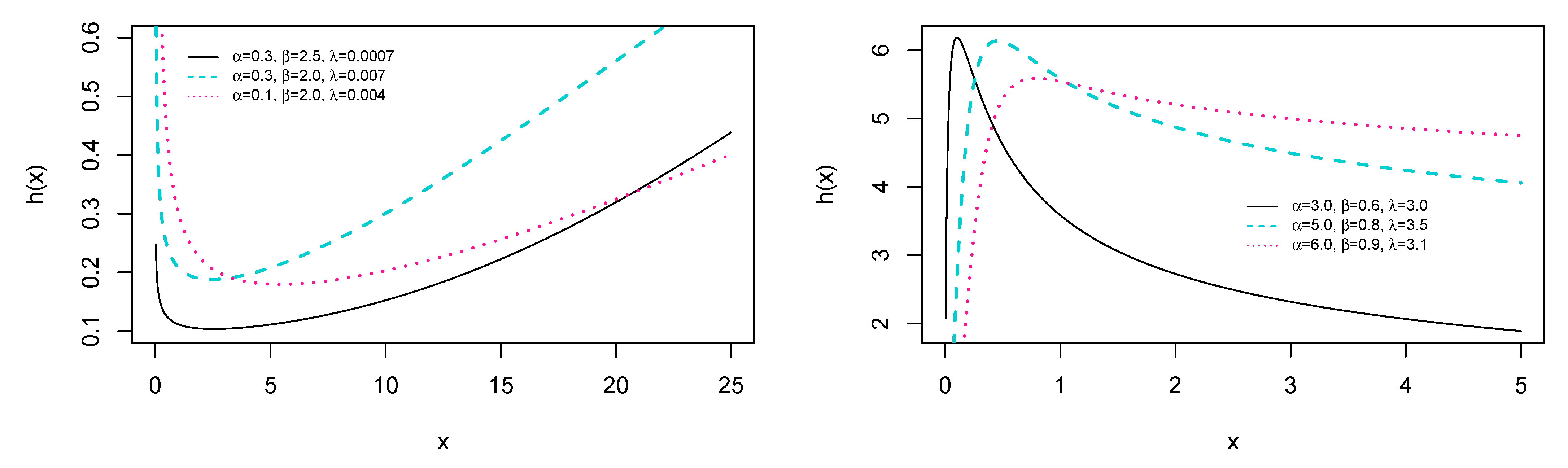
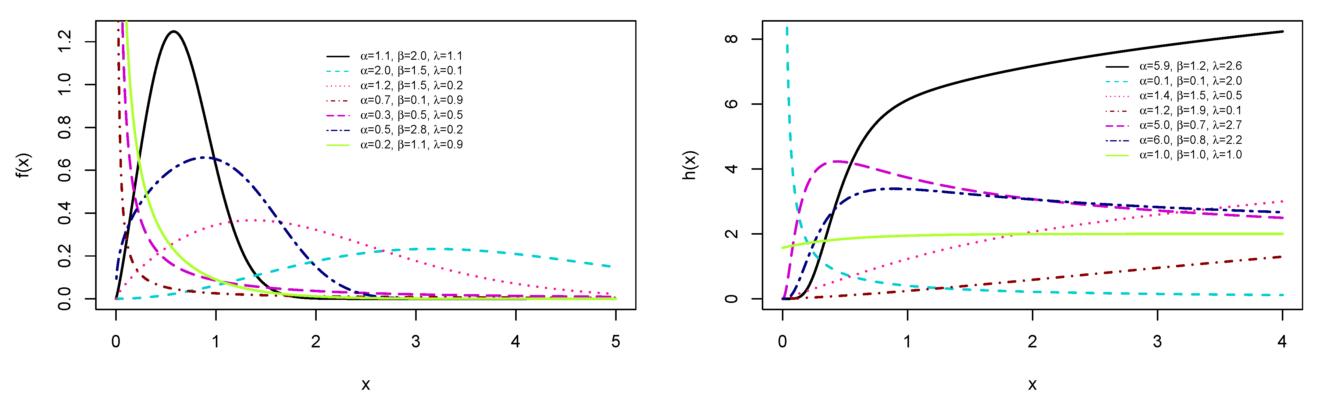
4. The ES Weibull Distribution
- As , we haveand
- As , we haveand
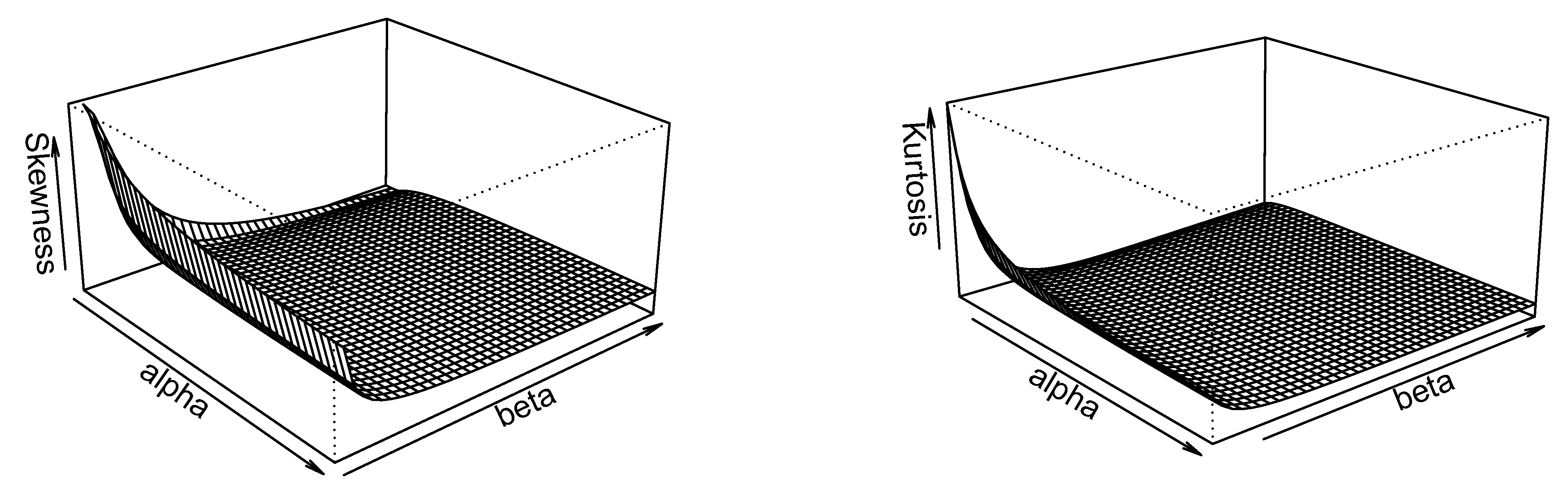
4.1. Quantile and Moments
4.2. Moments of Residual Life
4.3. Order Statistics and Asymptotic
5. Parameter Estimation
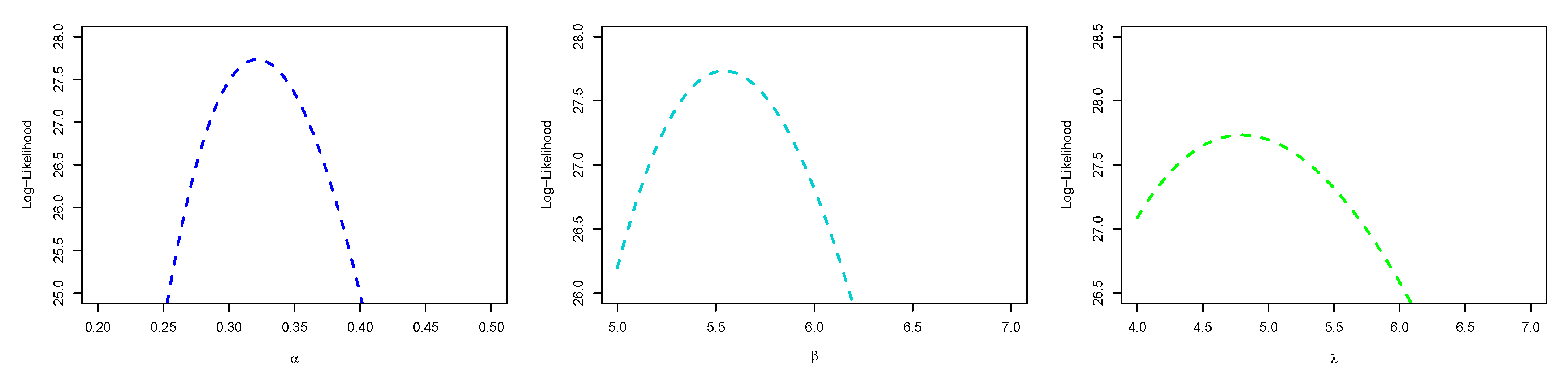
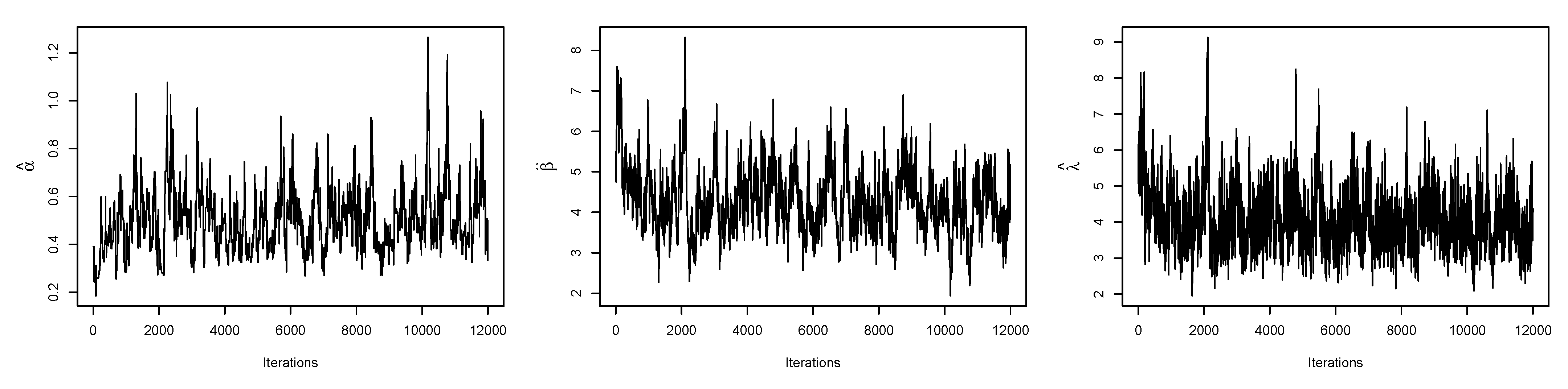
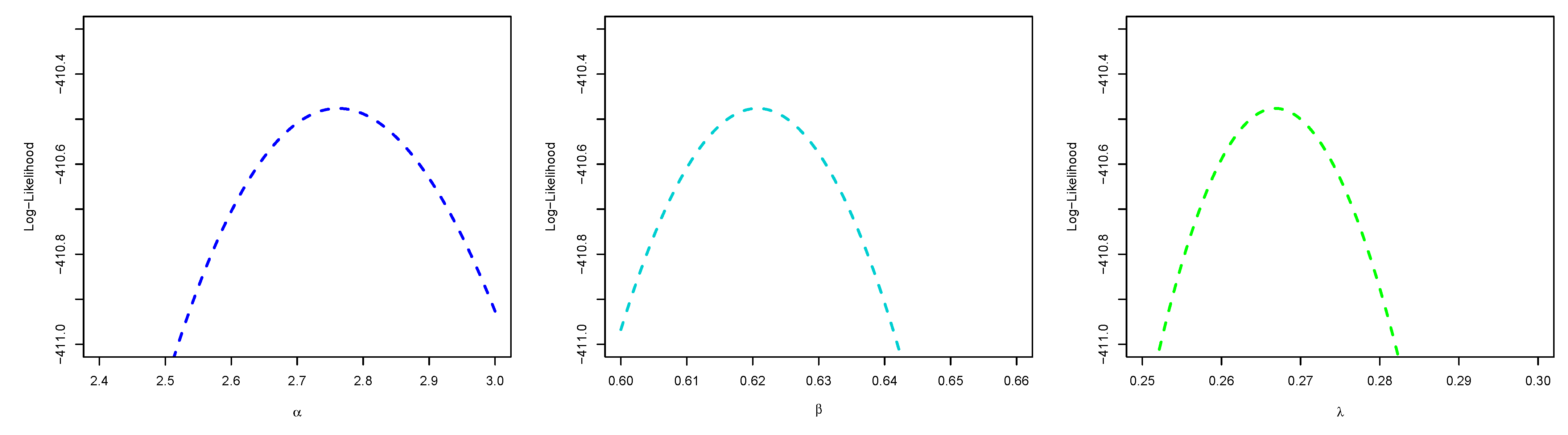
5.1. Maximum Likelihood Estimation
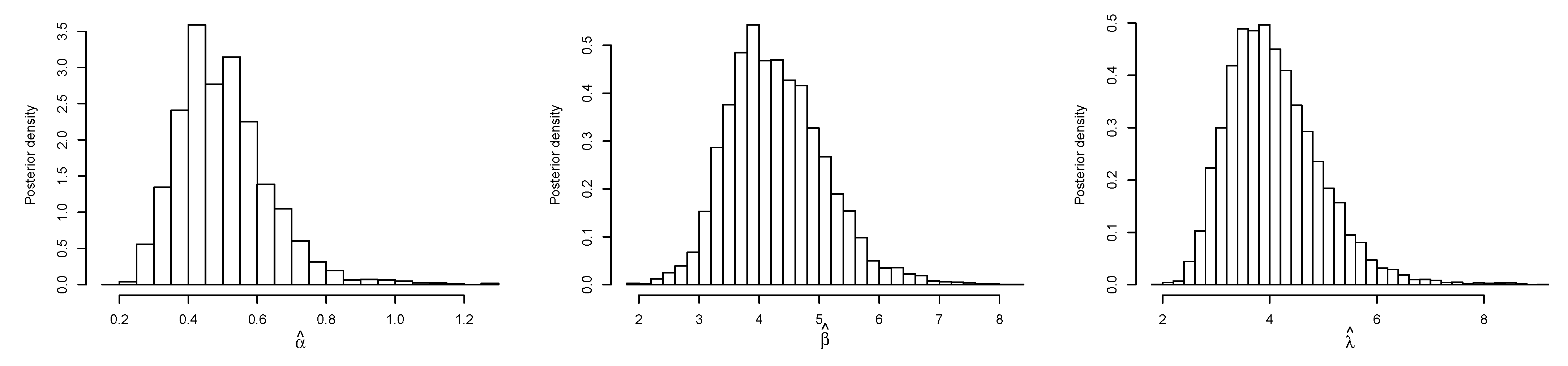
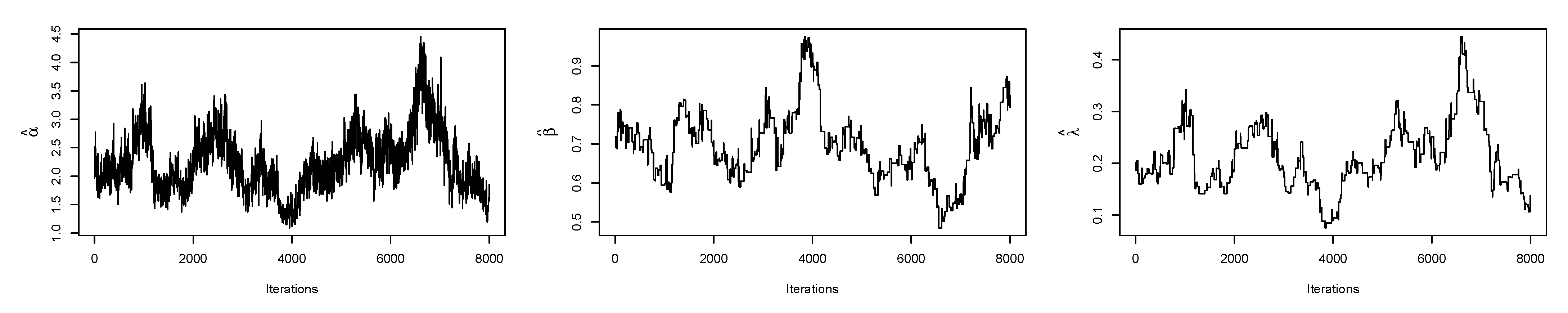
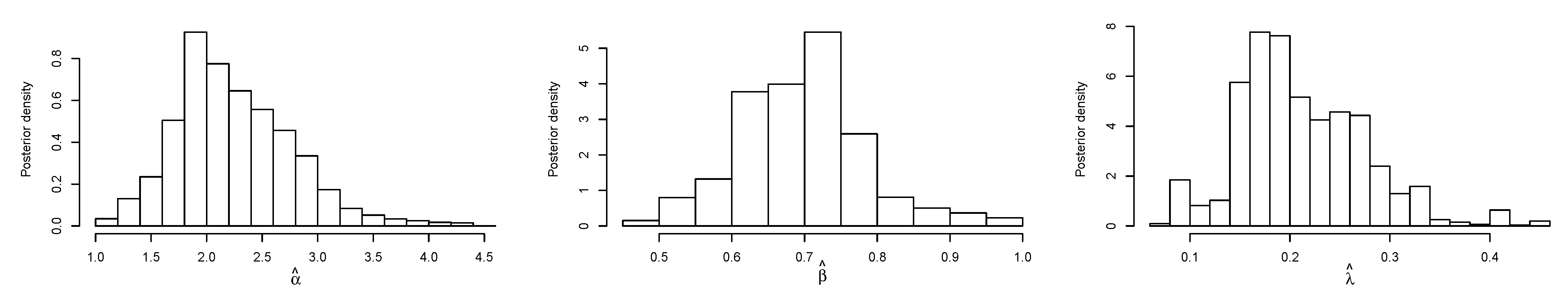
5.2. Bayes Estimation
- Start by initial guess ,
- Set ,
- Apply the MH algorithm to generate from ,
- Apply the MH algorithm to generate from ,
- Apply the MH algorithm to generate from ,
- Set ,
- Repeat step 3 to 6, T times.
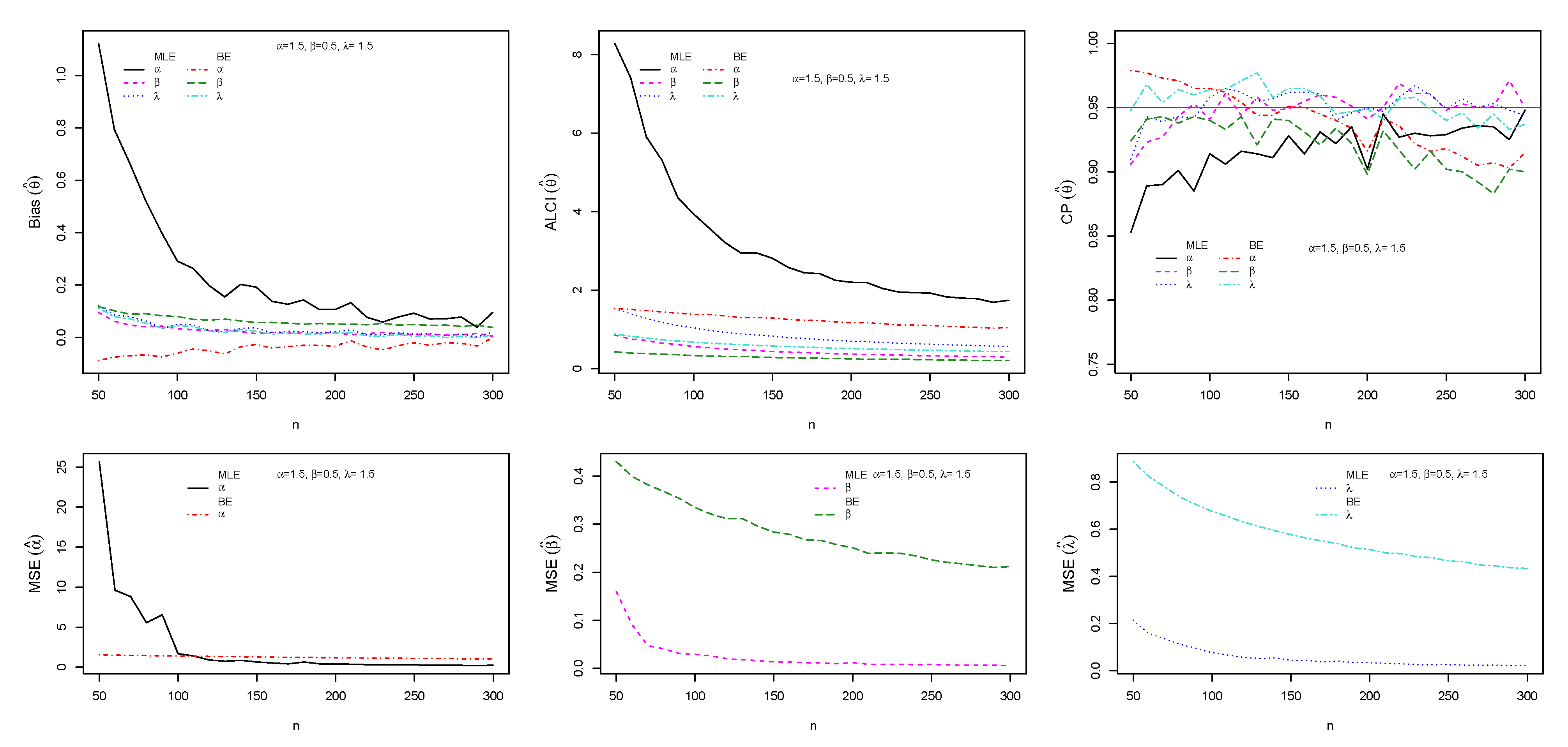
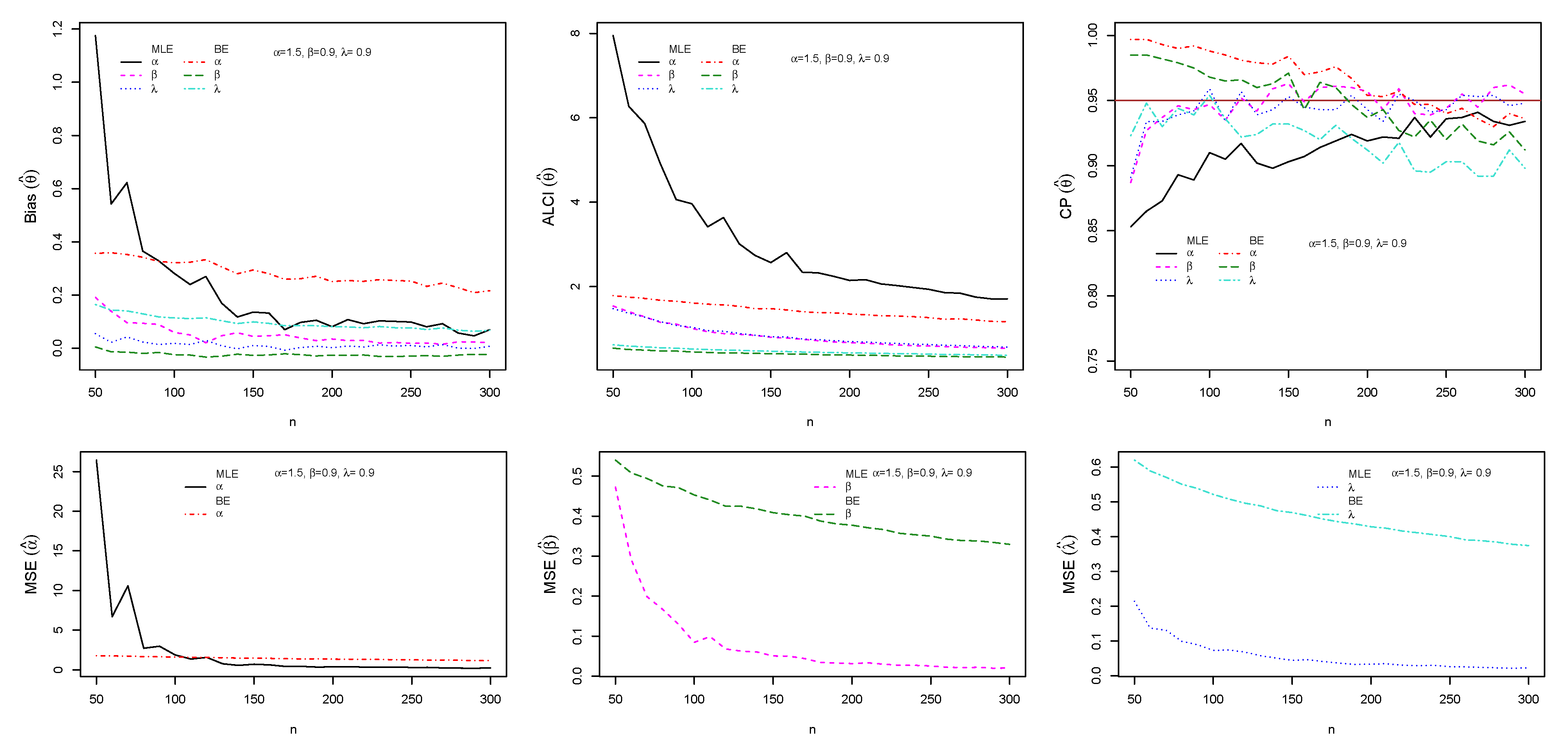
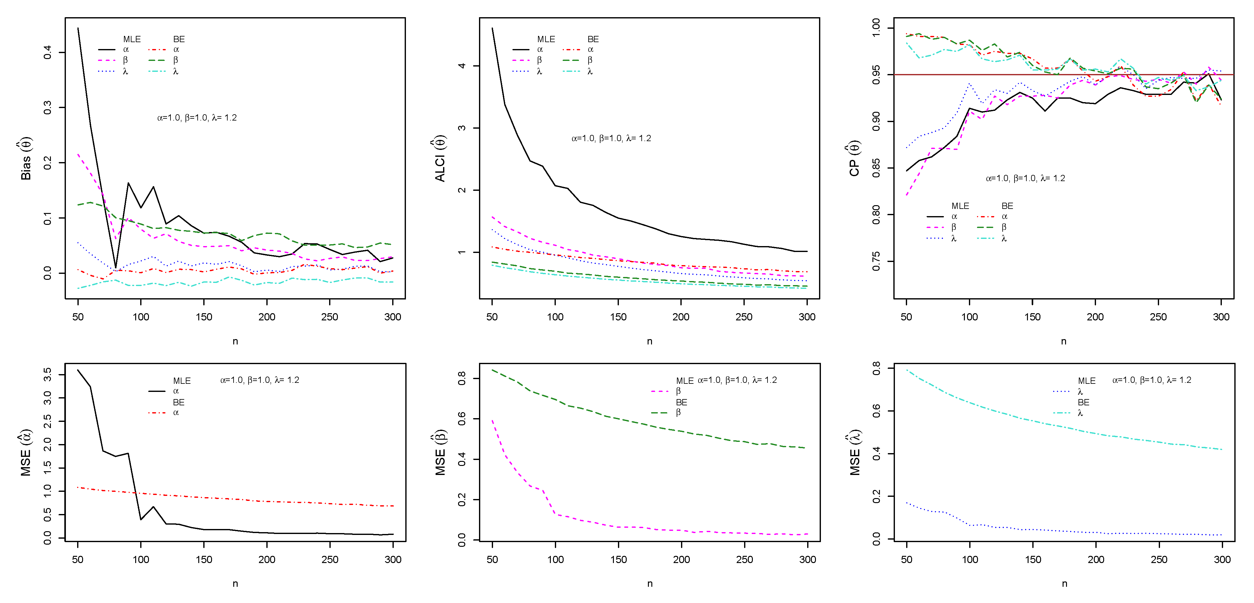
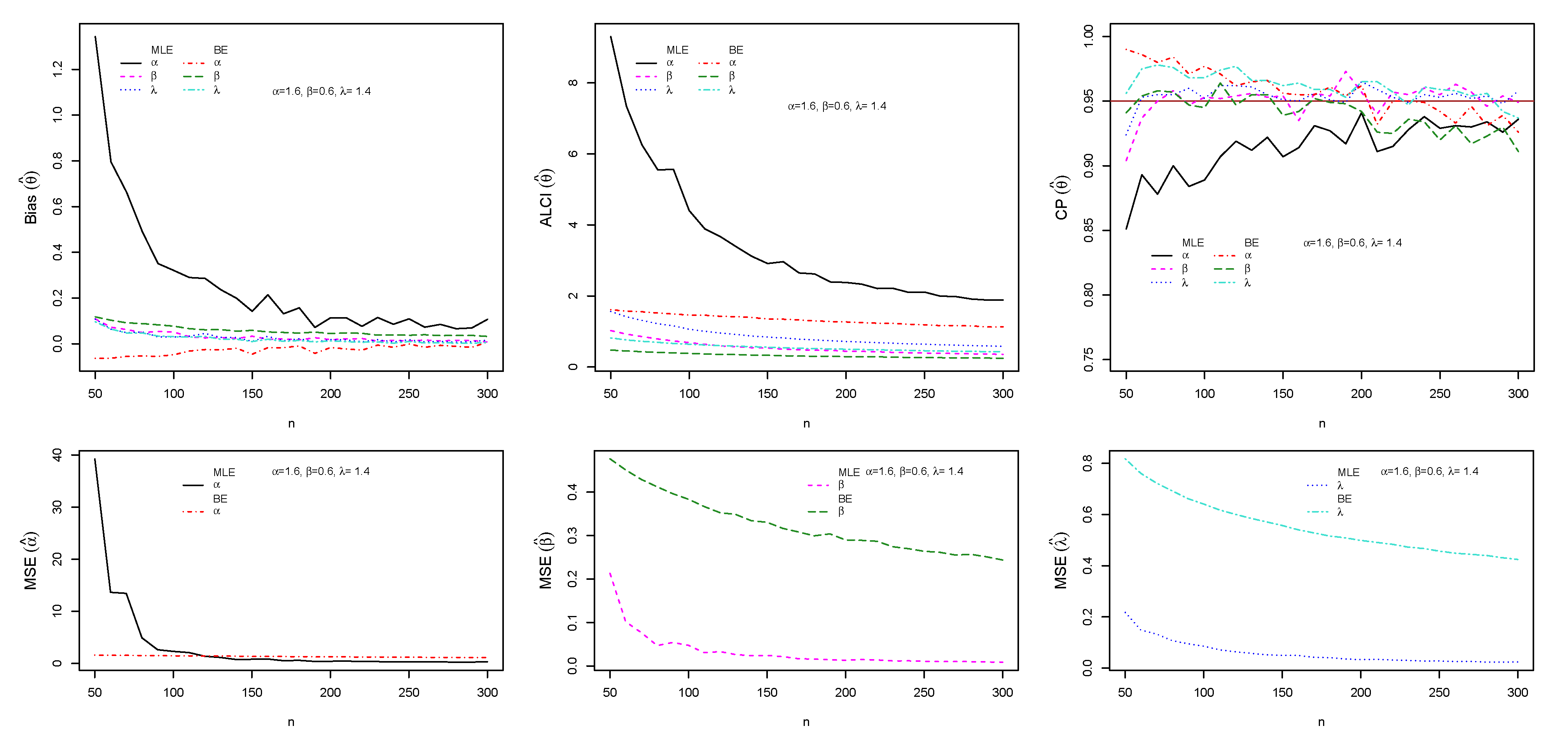
5.3. Simulation Study I
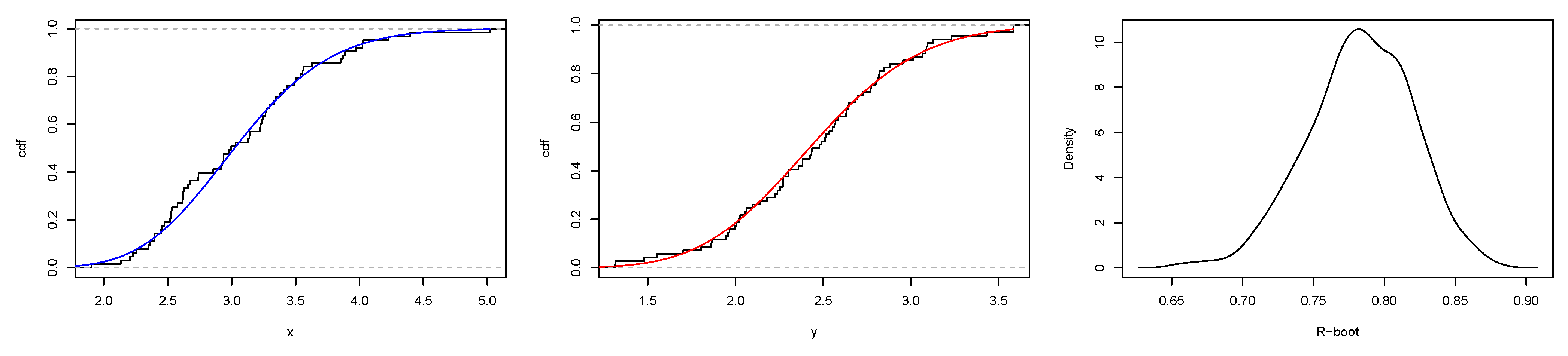
5.4. Estimation of the Stress-Strength Reliability from the ESW Distribution
5.4.1. Maximum Likelihood Estimation of R
5.4.2. Bootstrap CIs for R
- We generate a sample of values from the distribution, and an independent sample of values from the distribution.
- We generate independent bootstrap samples of values and using sampling with replacement from the first step in above. Based on the bootstrap sample, we compute the MLE of , say , then compute the corresponding MLE of R, say .
- In order to get a set of bootstrap samples of R, repeat step 2 to 3 B-times. We consider the samples ordered in an increasing order, say , .
- Percentile bootstrap CI:Let be the percentile of , . That iswhere denotes the standard indicator function. A Bp CI of R is given as
- Student’s t bootstrap CI:Let us setand be the percentile of , , such thatWith these tools, a CI of R is given as
5.4.3. Simulation Study II
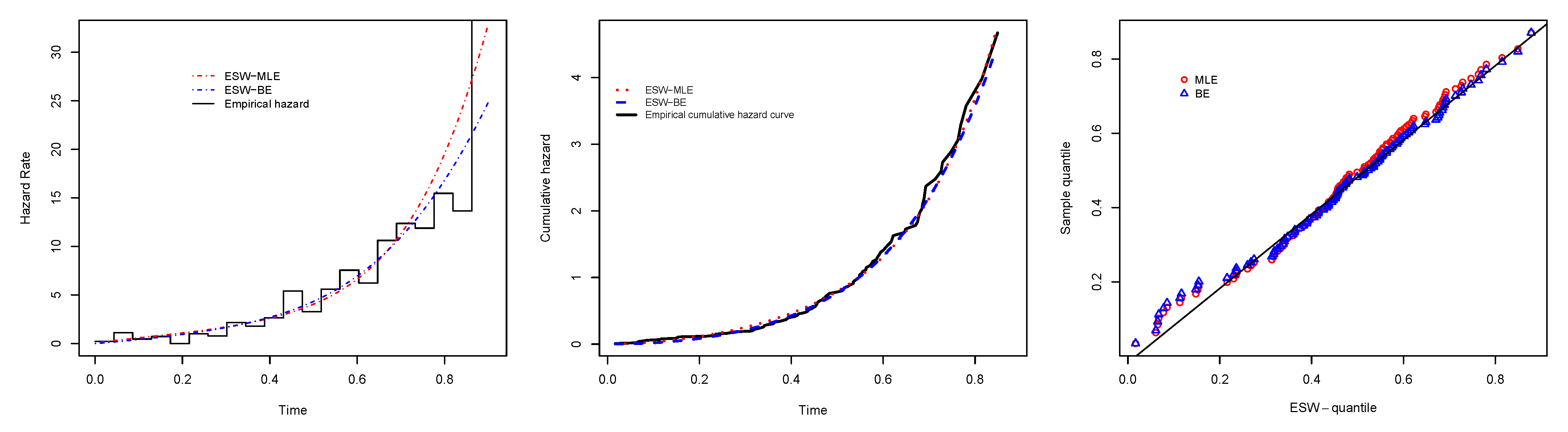
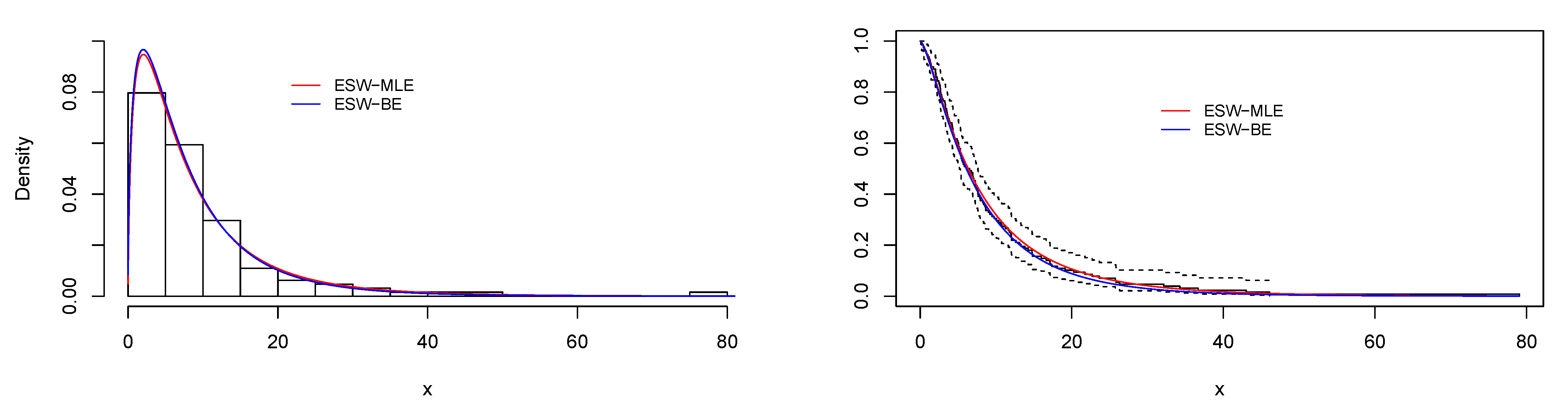
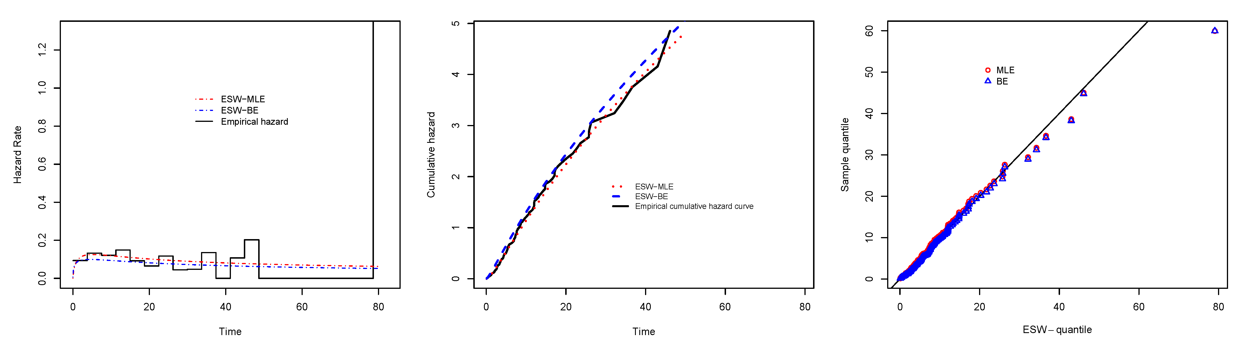
6. Application
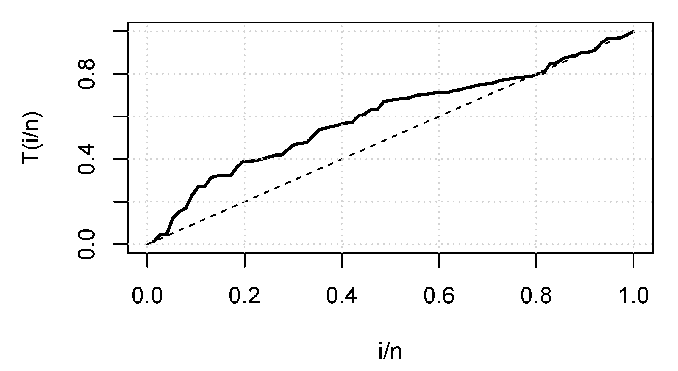
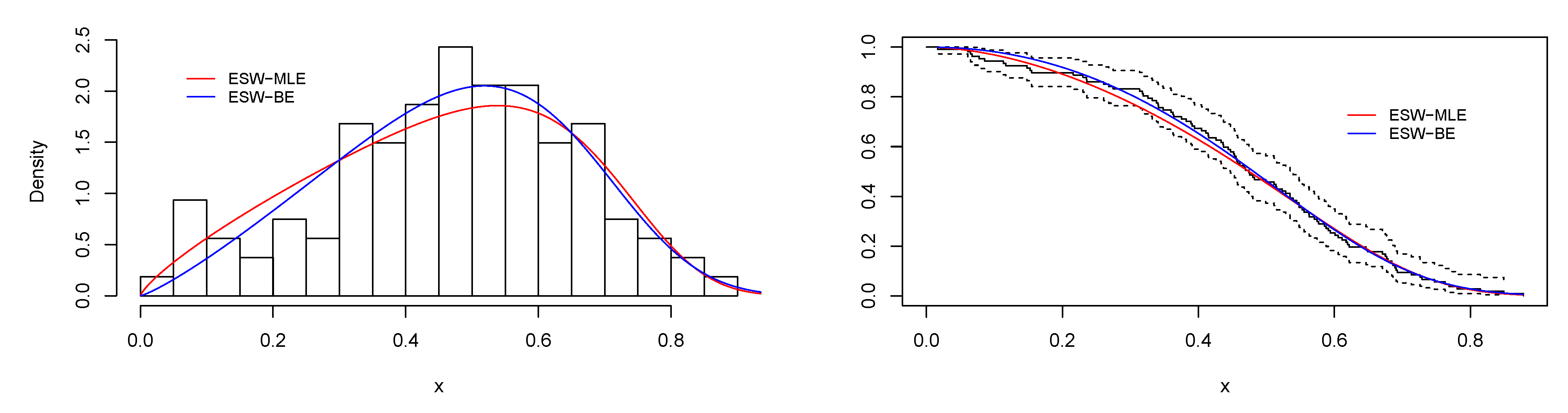
6.1. Real Data Application I
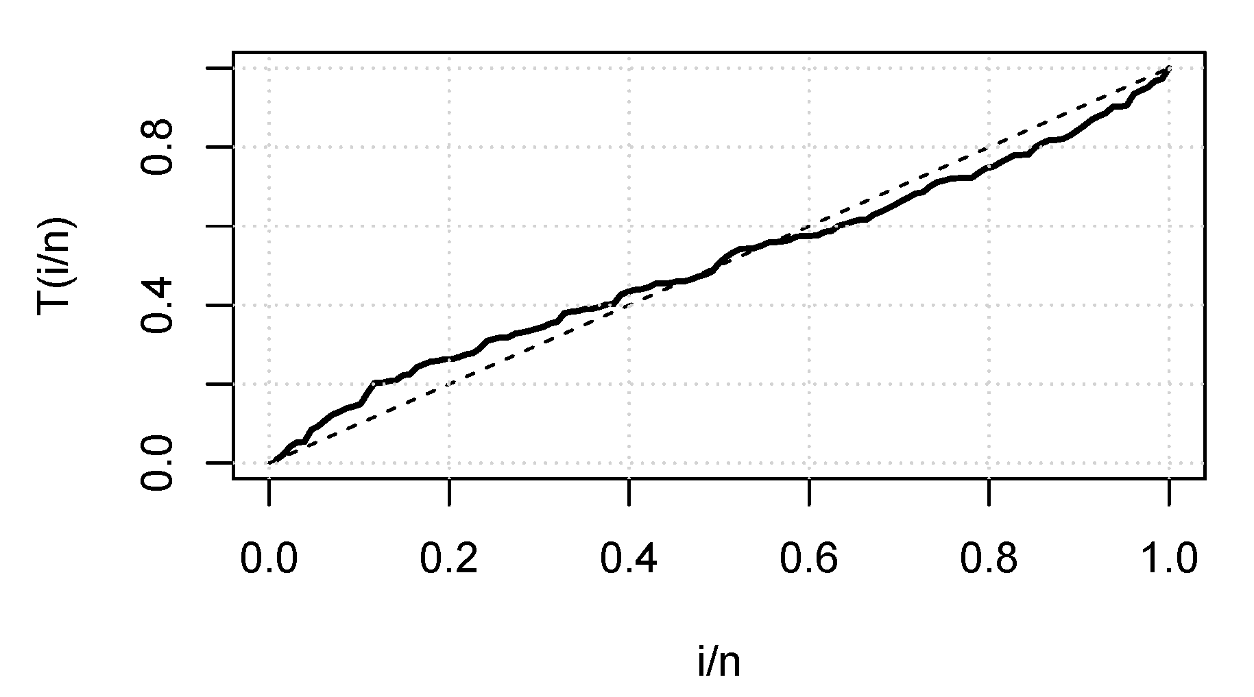
6.2. Real Data Application II
6.3. Real Data Application III
7. Conclusions
Author Contributions
Funding
Institutional Review Board Statement
Informed Consent Statement
Data Availability Statement
Acknowledgments
Conflicts of Interest
References
- Evans, M.; Hastings, N.; Peacock, B. Statistical Distributions; IOP Publishing: Bristol, UK, 2001. [Google Scholar]
- Kent, J.T.; Tyler, D.E. Maximum likelihood estimation for the wrapped Cauchy distribution. J. Appl. Stat. 1988, 15, 247–254. [Google Scholar] [CrossRef]
- Fisher, N.I. Statistical Analysis of Directional Data; Cambridge University Press: Cambridge, UK, 1993. [Google Scholar]
- Nadarajah, S.; Kotz, S. Beta trigonometric distributions. Port. Econ. J. 2006, 5, 207–224. [Google Scholar] [CrossRef]
- Al-Faris, R.Q.; Khan, S. Sine square distribution: A new statistical model based on the sine function. J. Appl. Probab. Stat. 2008, 3, 163–173. [Google Scholar]
- Kharazmi, O.; Saadatinik, A. Hyperbolic cosine-F family of distributions with an application to exponential distribution. Gazi Univ. J. Sci. 2016, 29, 811–829. [Google Scholar]
- Kumar, D.; Singh, U.; Singh, S.K. A new distribution using sine function-its application to bladder cancer patients data. J. Stat. Appl. Probab. 2015, 4, 417. [Google Scholar]
- Chesneau, C.; Bakouch, H.S.; Hussain, T. A new class of probability distributions via cosine and sine functions with applications. Commun. Stat. Simul. Comput. 2019, 48, 2287–2300. [Google Scholar] [CrossRef]
- Mahmood, Z.; Chesneau, C.; Tahir, M.H. A new sine-G family of distributions: Properties and applications. Bull. Comput. Appl. Math. 2019, 7, 53–81. [Google Scholar]
- Jamal, F.; Chesneau, C. A new family of polyno-expo-trigonometric distributions with applications. Infin. Dimens. Anal. Quantum Probab. Relat. Top. 2019, 22, 1950027. [Google Scholar] [CrossRef] [Green Version]
- Bakouch, H.S.; Chesneau, C.; Leao, J. A new lifetime model with a periodic hazard rate and an application. J. Stat. Comput. Simul. 2018, 88, 2048–2065. [Google Scholar] [CrossRef]
- Abate, J.; Choudhury, G.L.; Lucantoni, D.M.; Whitt, W. Asymptotic analysis of tail probabilities based on the computation of moments. Ann. Appl. Probab. 1995, 5, 983–1007. [Google Scholar] [CrossRef]
- Brychkov, Y.A. Power expansions of powers of trigonometric functions and series containing Bernoulli and Euler polynomials. Integral Transform. Spec. Funct. 2009, 20, 797–804. [Google Scholar] [CrossRef]
- Gupta, R.C.; Gupta, P.L.; Gupta, R.D. Modeling failure time data by Lehman alternatives. Commun. Stat. Theory Methods 1998, 27, 887–904. [Google Scholar] [CrossRef]
- Gradshteyn, I.; Ryzhik, I.; Jeffrey, A.; Zwillinger, D. Table of Integrals, Series and Products, 7th ed.; Academic Press: New York, NY, USA, 2007. [Google Scholar]
- Kotz, S.; Pensky, M. The Stress-Strength Model and Its Generalizations: Theory and Applications; World Scientific: Singapore, 2003. [Google Scholar]
- Asgharzadeh, A.; Valiollahi, R.; Raqab, M.Z. Estimation of the stress–strength reliability for the generalized logistic distribution. Stat. Methodol. 2013, 15, 73–94. [Google Scholar] [CrossRef]
- Barbiero, A. Confidence intervals for reliability of stress-strength models in the normal case. Commun. Stat. Simul. Comput. 2011, 40, 907–925. [Google Scholar] [CrossRef]
- Guo, H.; Krishnamoorthy, K. New approximate inferential methods for the reliability parameter in a stress–strength model: The normal case. Commun. Stat. Theory Methods 2004, 33, 1715–1731. [Google Scholar] [CrossRef]
- Baklizi, A.; El-Masri, A.E.Q. Shrinkage estimation of p(x < y) in the exponential case with common location parameter. Metrika 2004, 59, 163–171. [Google Scholar]
- Kundu, D.; Gupta, R.D. Estimation of p[y < x] for generalized exponential distribution. Metrika 2005, 61, 291–308. [Google Scholar]
- Nadarajah, S.; Bagheri, S.; Alizadeh, M.; Samani, E.B. Estimation of the stress strength parameter for the generalized exponential-Poisson distribution. J. Test. Eval. 2018, 46, 2184–2202. [Google Scholar] [CrossRef]
- Muhammad, M. Poisson-odd generalized exponential family of distributions: Theory and applications. Hacet. J. Math. Stat. 2016, 47, 1652–1670. [Google Scholar] [CrossRef]
- Shrahili, M.; Elbatal, I.; Muhammad, I.; Muhammad, M. Properties and applications of beta Erlang-truncated exponential distribution. J. Math. Comput. Sci. (JMCS) 2021, 22, 16–37. [Google Scholar] [CrossRef]
- Muhammad, M.; Liu, L. A new extension of the generalized half logistic distribution with applications to real data. Entropy 2019, 21, 339. [Google Scholar] [CrossRef] [Green Version]
- Muhammad, I.; Wang, X.; Li, C.; Yan, M.; Chang, M. Estimation of the reliability of a stress–strength system from Poisson half logistic distribution. Entropy 2020, 22, 1307. [Google Scholar] [CrossRef]
- Krishnamoorthy, K.; Lin, Y. Confidence limits for stress–strength reliability involving Weibull models. J. Stat. Plan. Inference 2010, 140, 1754–1764. [Google Scholar] [CrossRef]
- Kundu, D.; Gupta, R.D. Estimation of p[y < x] for Weibull distributions. IEEE Trans. Reliab. 2006, 55, 270–280. [Google Scholar]
- Asgharzadeh, A.; Valiollahi, R.; Raqab, M.Z. Stress-strength reliability of Weibull distribution based on progressively censored samples. Sort-Stat. Oper. Res. Trans. 2011, 35, 103–124. [Google Scholar]
- Arnold, B.C.; Balakrishnan, N.; Nagaraja, H.N. A First Course in Order Statistics; Wiley: New York, NY, USA, 1992; Volume 54. [Google Scholar]
- Muhammad, M. A generalization of the Burr XII-poisson distribution and its applications. J. Stat. Appl. Probab. 2016, 5, 29–41. [Google Scholar] [CrossRef]
- Muhammad, M.; Liu, L. A new three parameter lifetime model: The complementary poisson generalized half logistic distribution. IEEE Access 2021, 9, 60089–60107. [Google Scholar] [CrossRef]
- Meredith, M.; Kruschke, J. Hdinterval: Highest (Posterior) Density Intervals. R Package Version 013. 2016. Available online: https://CRAN.R-project.org/package=HDInterval (accessed on 13 September 2021).
- Metropolis, N.; Rosenbluth, A.W.; Rosenbluth, M.N.; Teller, A.H.; Teller, E. Equation of state calculations by fast computing machines. J. Chem. Phys. 1953, 21, 1087–1092. [Google Scholar] [CrossRef] [Green Version]
- Hastings, W.K. Monte carlo sampling methods using Markov chains and their applications. Biometrika 1970, 57, 97–109. [Google Scholar] [CrossRef]
- Gelf, A.E.; Smith, A.F. Sampling-based approaches to calculating marginal densities. J. Am. Stat. Assoc. 1990, 85, 398–409. [Google Scholar]
- Chen, M.H.; Shao, Q.M. Monte Carlo estimation of Bayesian credible and HPD intervals. J. Comput. Graph. Stat. 1999, 8, 69–92. [Google Scholar]
- R Core Team. A Language and Environment for Statistical Computing; R Foundation for Statistical Computing: Vienna, Austria, 2019. [Google Scholar]
- Henningsen, A.; Toomet, O. maxlik: A package for maximum likelihood estimation in R. Comput. Stat. 2011, 26, 443–458. [Google Scholar] [CrossRef]
- Friendly, M.; Fox, J.; Chalmers, P.; Monette, G.; Sanchez, G.; Friendly, M.M. Package Matlib. 2016. Available online: https://cran.r-project.org/web/packages/matlib/index.html (accessed on 13 September 2021).
- Tibshirani, R.J.; Efron, B. An Introduction to the Bootstrap; Monographs on Statistics and Applied Probability; Chapman & Hall: New York, NY, USA, 1993; Volume 57, 436p. [Google Scholar]
- Gupta, R.D.; Kundu, D. Theory & methods: Generalized exponential distributions. Aust. N. Z. J. Stat. 1999, 41, 173–188. [Google Scholar]
- Lovric, M. International Encyclopedia of Statistical Science; Springer: Berlin/Heidelberg, Germany, 2011. [Google Scholar]
- Barreto-Souza, W.; Cribari-Neto, F. A generalization of the exponential-Poisson distribution. Stat. Probab. Lett. 2009, 79, 2493–2500. [Google Scholar] [CrossRef] [Green Version]
- Muhammad, M.; Yahaya, M.A. The half logistic-Poisson distribution. Asian J. Math. Appl. 2017, 2017, 126000416. [Google Scholar]
- Abdul-Moniem, I.B. Exponentiated Nadarajah and Haghighi exponential distribution. Int. J. Math. Anal. Appl. 2015, 2, 68–73. [Google Scholar]
- Lemonte, A.J. A new exponential-type distribution with constant, decreasing, increasing, upside-down bathtub and bathtub-shaped failure rate function. Comput. Stat. Data Anal. 2013, 62, 149–170. [Google Scholar] [CrossRef]
- DeGusmao, F.R.; Ortega, E.M.; Cordeiro, G.M. The generalized inverse Weibull distribution. Stat. Pap. 2011, 52, 591–619. [Google Scholar] [CrossRef]
- Cordeiro, G.M.; dos Santos Brito, R. The beta power distribution. Braz. J. Probab. Stat. 2012, 26, 88–112. [Google Scholar]
- Lee, E.T.; Wang, J. Statistical Methods for Survival Data Analysis; John Wiley & Sons: Hoboken, NJ, USA, 2003; Volume 476. [Google Scholar]
- Muhammad, M. Generalized half-logistic Poisson distributions. Commun. Stat. Appl. Methods 2017, 24, 353–365. [Google Scholar]
- Bader, M.; Priest, A. Statistical aspects of fibre and bundle strength in hybrid composites. In Proceedings of the Fourth International Conference on Composite Materials, Tokyo, Japan, 25–28 October 1982; Progress in Science and Engineering of Composites. pp. 1129–1136. [Google Scholar]


| R | ||||||
|---|---|---|---|---|---|---|
| (0.8, 0.7, 0.5, 0.6, 0.5) | 0.5182 | (20, 20) | 0.5187 (0.0939) | 0.0088 (0.0006) | 0.4153 (0.93) | 0.4971 (0.94) |
| (30, 20) | 0.5233 (0.0778) | 0.0061 (0.0052) | 0.3238 (0.94) | 0.3544 (0.94) | ||
| (40, 40) | 0.5191 (0.0585) | 0.0034 (0.0010) | 0.2323 (0.94) | 0.2341 (0.94) | ||
| (40, 60) | 0.5181 (0.0544) | 0.0030 () | 0.2115 (0.95) | 0.2108 (0.95) | ||
| (60, 60) | 0.5189 (0.0496) | 0.0025 (0.0007) | 0.1871 (0.94) | 0.1876 (0.94) | ||
| (0.8, 0.7, 1.2, 1.0, 0.6) | 0.5555 | (20, 20) | 0.5080 (0.1827) | 0.0356 (−0.0475) | 0.6756 (0.94) | 0.9333 (0.89) |
| (30, 20) | 0.5263 (0.1411) | 0.0208 (−0.0292) | 0.6082 (0.94) | 0.8711 (0.92) | ||
| (40, 40) | 0.5511 (0.0792) | 0.0063 (−0.0044) | 0.4348 (0.94) | 0.6333 (0.96) | ||
| (40, 60) | 0.5546 (0.0665) | 0.0044 (−0.0009) | 0.3434 (0.94) | 0.4769 (0.96) | ||
| (60, 60) | 0.5564 (0.0509) | 0.0026 (0.0008) | 0.2636 (0.95) | 0.3413 (0.95) | ||
| (0.9, 0.5, 0.6, 0.8, 0.7) | 0.5972 | (20, 20) | 0.5970 (0.0893) | 0.0080 (−0.0021) | 0.4574 (0.94) | 0.5967 (0.95) |
| (30, 20) | 0.5988 (0.0748) | 0.0056 (0.0015) | 0.3406 (0.94) | 0.4051 (0.95) | ||
| (40, 40) | 0.5976 (0.0575) | 0.0033 (0.0004) | 0.2283 (0.95) | 0.2408 (0.95) | ||
| (40, 60) | 0.5986 (0.537) | 0.0029 (0.0013) | 0.2053 (0.93) | 0.2081 (0.93) | ||
| (60, 60) | 0.5997 (0.0479) | 0.0023 (0.0025) | 0.1784 (0.94) | 0.1793 (0.94) | ||
| (0.6, 0.5, 0.9, 0.9, 0.7) | 0.5455 | (20, 20) | 0.5278 (0.1235) | 0.0155 (−0.0176) | 0.5598 (0.94) | 0.7735 (0.95) |
| (30, 20) | 0.5378 (0.0882) | 0.0078 (−0.0076) | 0.4385 (0.94) | 0.5898 (0.96) | ||
| (40, 40) | 0.5467 (0.0618) | 0.0038 (0.0012) | 0.2780 (0.94) | 0.3333 (0.94) | ||
| (40, 60) | 0.5441 (0.0555) | 0.0031 (−0.0013) | 0.2554 (0.94) | 0.3065 (0.94) | ||
| (60, 60) | 0.5458 (0.0480) | 0.0023 (0.0004) | 0.1870 (0.93) | 0.1940 (0.93) | ||
| (2.5, 1.3, 2.0, 1.1, 1.4) | 0.7736 | (20, 20) | 0.7233 (0.2232) | 0.05229 (−0.0503) | 0.7678 (0.95) | 1.1720 (0.88) |
| (30, 20) | 0.7481 (0.1661) | 0.0282 (−0.0256) | 0.6759 (0.94) | 1.0583 (0.93) | ||
| (40, 40) | 0.7594 (0.1162) | 0.0137 (−0.0142) | 0.4909 (0.95) | 0.7720 (0.95) | ||
| (40, 60) | 0.7707 (0.0819) | 0.0067 (−0.0030) | 0.4094 (0.94) | 0.6441 (0.93) | ||
| (60, 60) | 0.7757 (0.0530) | 0.0028 (0.0021) | 0.2846 (0.92) | 0.4186 (0.93) | ||
| (2.5, 0.5, 1.0, 2.6, 0.3) | 0.9084 | (20, 20) | 0.9074 (0.0668) | 0.0045 (−0.0010) | 0.3645 (0.90) | 0.5907 (0.91) |
| (30, 20) | 0.9073 (0.0627) | 0.0039 (−0.0011) | 0.2843 (0.92) | 0.4423 (0.93) | ||
| (40, 40) | 0.9106 (0.0321) | 0.0010 (0.0022) | 0.1314 (0.90) | 0.1574 (0.91) | ||
| (40, 60) | 0.9108 (0.0305) | 0.0009 (0.0024) | 0.1111 (0.90) | 0.1204 (0.90) | ||
| (60, 60) | 0.9092 (0.0259) | 0.0007 (0.0008) | 0.0969 (0.93) | 0.1029 (0.93) | ||
| (3.8, 1.2, 1.5, 1.2, 1.1) | 0.7787 | (20, 20) | 0.7567 (0.1584) | 0.0255 (−0.0219) | 0.6621 (0.94) | 1.0187 (0.92) |
| (30, 20) | 0.7743 (0.1167) | 0.0136 (−0.0044) | 0.5471 (0.91) | 0.8355 (0.91) | ||
| (40, 40) | 0.7594 (0.1163) | 0.0137 (−0.0142) | 0.4909 (0.95) | 0.7720 (0.95) | ||
| (40, 60) | 0.7783 (0.0601) | 0.0036 (−0.0004) | 0.3099 (0.94) | 0.4329 (0.95) | ||
| (60, 60) | 0.7791 (0.0412) | 0.0017 (0.0005) | 0.1740 (0.93) | 0.1969 (0.93) | ||
| (1.0, 1.0, 1.0, 1.0, 1.0) | 0.5000 | (20, 20) | 0.4738 (0.1447) | 0.0216 (−0.0262) | 0.5975 (0.94) | 0.8229 (0.92) |
| (30, 20) | 0.4854 (0.1195) | 0.0145 (−0.0146) | 0.5135 (0.94) | 0.7150 (0.94) | ||
| (40, 40) | 0.4940 (0.0841) | 0.0071 (−0.0060) | 0.4511 (0.95) | 0.6473 (0.96) | ||
| (40, 60) | 0.4964 (0.0665) | 0.0044 (−0.0036) | 0.3099 (0.94) | 0.4093 (0.95) | ||
| (60, 60) | 0.4993 (0.0464) | 0.0022 (−0.0007) | 0.2297 (0.94) | 0.2780 (0.96) |
| Model | AIC | BIC | CAIC | KS | AD | CvM | |||||
|---|---|---|---|---|---|---|---|---|---|---|---|
| ESW | 0.3216 | 5.5424 | 4.7906 | - | 27.732 | −49.464 | −41.446 | −49.231 | 0.0734 | 0.5305 | 0.0836 |
| (0.2557, 0.3875) | (5.3049, 5.7799) | (4.5531, 5.0282) | (0.6113) | ||||||||
| ESW | 0.5021 | 4.2903 | 4.0846 | - | - | - | - | - | 0.0573 | 0.5825 | 0.0871 |
| (0.2604, 0.7447) | (2.8145, 5.8670) | (2.6074, 5.7682) | (0.8744) | ||||||||
| ESE | 3.3101 | - | 2.1712 | - | 6.596 | −9.191 | −3.846 | −9.076 | 0.1418 | 4.0970 | 0.6751 |
| (2.3421, 4.2782) | (1.8087, 2.5336) | (0.0271) | |||||||||
| SW | - | 2.4894 | 2.8311 | - | 22.378 | −40.754 | −35.409 | −40.639 | 0.0766 | 1.3299 | 0.2003 |
| (2.0912, 2.8857) | (2.0695, 3.5926) | (0.5559) | |||||||||
| W | - | 2.6012 | 5.3818 | - | 21.348 | −38.695 | −33.349 | −38.580 | 0.0832 | 1.5126 | 0.2307 |
| (2.1896, 3.0128) | (3.8514, 6.9122) | (0.4487) | |||||||||
| GE | 3.7139 | - | 4.2007 | - | 5.039 | −6.078 | −0.732 | −5.962 | 0.1477 | 4.3696 | 0.7257 |
| (2.6102, 4.8176) | (3.4729, 4.9284) | (0.0188) | |||||||||
| GR | 2.1189 | - | - | 1.2567 | 18.155 | −32.311 | −26.195 | −32.195 | 0.1178 | 2.1579 | 0.3371 |
| (2.6102, 4.8176) | (3.4730, 4.9284) | (0.1026) | |||||||||
| GEP | 4.2690 | 3.7540 | 4.1128 | - | 5.0158 | −4.0316 | 3.9869 | −3.7986 | 0.1544 | 4.3799 | 0.7276 |
| (4.2439, 4.2947) | (3.0422, 4.4662) | (0, 0.0061) | (0.0121) | ||||||||
| HLP | 5.7570 | - | −4.9618 | - | 17.877 | −31.754 | −26.409 | −31.639 | 0.0916 | 1.9932 | 0.3015 |
| (5.0236, 6.4923) | (−6.4447, −3.4788) | (0.3302) | |||||||||
| ENH | 32.5264 | 2.3595 | 0.0608 | - | 21.0381 | −36.076 | −28.058 | −35.843 | 0.2995 | 1.3831 | 0.2104 |
| (0, 74.2789) | (1.7901, 2.9288) | (0, 0.1409) | () |
| Model | AIC | BIC | CAIC | KS | AD | CvM | ||||||
|---|---|---|---|---|---|---|---|---|---|---|---|---|
| ESW | 2.7619 | 0.6207 | 0.2668 | - | - | −410.476 | 826.95 | 835.508 | 827.146 | 0.0435 | 0.2594 | 0.0394 |
| (0.3971, 5.1267) | (0.3765, 0.8649) | (0.0132, 0.5204) | (0.9688) | |||||||||
| ESW | 2.2475 | 0.6275 | 0.2614 | - | - | - | - | - | - | 0.0507 | 0.2952 | 0.0468 |
| (1.2466, 3.2377) | (0.5272, 0.8899) | (0.0752, 0.3236 ) | (0.8967) | |||||||||
| ESE | 1.1164 | - | 0.0639 | - | - | −413.915 | 831.830 | 837.535 | 831.926 | 0.0786 | 0.8107 | 0.1365 |
| (0.8549, 1.3779) | (0.0504, 0.0774) | (0.4070) | ||||||||||
| SW | - | 0.9920 | 0.0611 | - | - | −414.325 | 832.650 | 838.354 | 832.746 | 0.0699 | 0.8312 | 0.1400 |
| (0.8644, 1.1196) | (0.0377, 0.0844) | (0.5581) | ||||||||||
| W | - | 1.0476 | 0.0939 | - | - | −414.087 | 832.174 | 837.878 | 832.270 | 0.0699 | 0.7815 | 0.1308 |
| (0.9152, 1.1800) | (0.0565, 0.1314) | (0.5123) | ||||||||||
| GR | 0.0476 | - | - | 0.3641 | - | −429.225 | 862.450 | 808.154 | 862.546 | 0.1551 | 2.7699 | 0.4729 |
| (0.9255, 1.5082) | (0.0945, 0.1477) | (0.0042) | ||||||||||
| GIW | 0.1988 | 0.7521 | - | - | 8.1915 | −444.000 | 894.002 | 902.558 | 894.195 | 0.1408 | 4.513 | 0.7414 |
| (0, 0.6116) | (0.6689, 0.8352) | (0, 20.8093) | (0.00125) | |||||||||
| HLP | 0.0555 | - | 4.0202 | - | - | −413.171 | 830.342 | 836.046 | 830.438 | 0.0954 | 0.3620 | 0.0606 |
| (0, 0.1237) | (0, 9.4418) | (0.1861) |
| R | ||||||||||
|---|---|---|---|---|---|---|---|---|---|---|
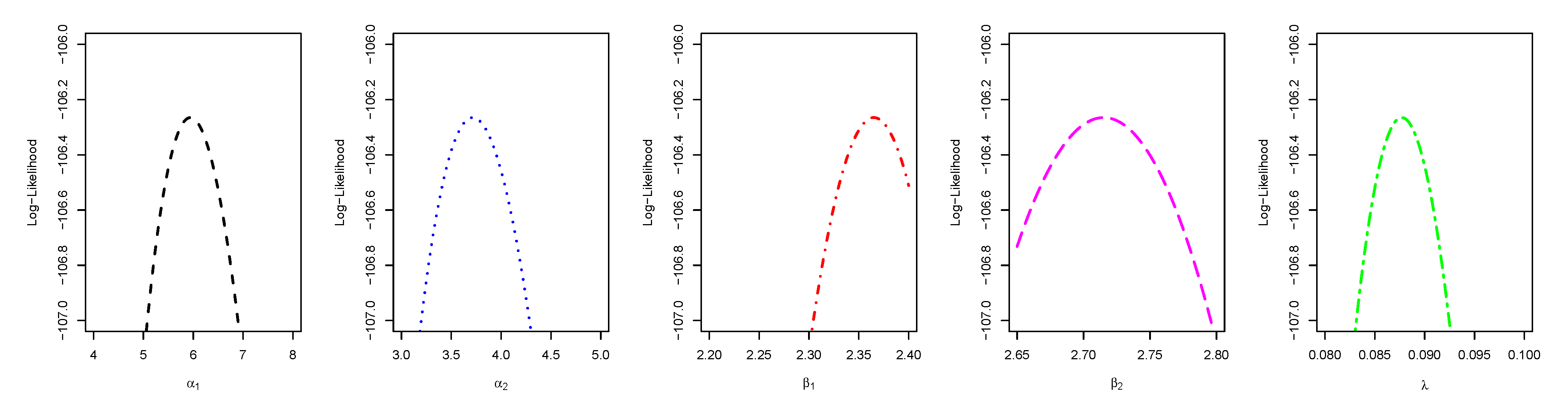
| 5.9420 | 3.7152 | 2.3651 | 2.7151 | 0.0877 | 106.265 | 0.0946 | 0.0485 | 0.7837 | (0.7073, 0.8524) | (0.7073, 0.8602) |
| (0.5921) | (0.9944) | 0.1451 | 0.1529 |
Publisher’s Note: MDPI stays neutral with regard to jurisdictional claims in published maps and institutional affiliations. |
© 2021 by the authors. Licensee MDPI, Basel, Switzerland. This article is an open access article distributed under the terms and conditions of the Creative Commons Attribution (CC BY) license (https://creativecommons.org/licenses/by/4.0/).
Share and Cite
Muhammad, M.; Alshanbari, H.M.; Alanzi, A.R.A.; Liu, L.; Sami, W.; Chesneau, C.; Jamal, F. A New Generator of Probability Models: The Exponentiated Sine-G Family for Lifetime Studies. Entropy 2021, 23, 1394. https://doi.org/10.3390/e23111394
Muhammad M, Alshanbari HM, Alanzi ARA, Liu L, Sami W, Chesneau C, Jamal F. A New Generator of Probability Models: The Exponentiated Sine-G Family for Lifetime Studies. Entropy. 2021; 23(11):1394. https://doi.org/10.3390/e23111394
Chicago/Turabian StyleMuhammad, Mustapha, Huda M. Alshanbari, Ayed R. A. Alanzi, Lixia Liu, Waqas Sami, Christophe Chesneau, and Farrukh Jamal. 2021. "A New Generator of Probability Models: The Exponentiated Sine-G Family for Lifetime Studies" Entropy 23, no. 11: 1394. https://doi.org/10.3390/e23111394
APA StyleMuhammad, M., Alshanbari, H. M., Alanzi, A. R. A., Liu, L., Sami, W., Chesneau, C., & Jamal, F. (2021). A New Generator of Probability Models: The Exponentiated Sine-G Family for Lifetime Studies. Entropy, 23(11), 1394. https://doi.org/10.3390/e23111394