Rate Distortion Function of Gaussian Asymptotically WSS Vector Processes

Abstract

In this paper, we obtain an integral formula for the rate distortion function (RDF) of any Gaussian asymptotically wide sense stationary (AWSS) vector process. Applying this result, we also obtain an integral formula for the RDF of Gaussian moving average (MA) vector processes and of Gaussian autoregressive MA (ARMA) AWSS vector processes.

1. Introduction

The present paper focuses on the derivation of a closed-form expression for the rate distortion function (RDF) of a wide class of vector processes. As stated in [1,2], there exist very few journal papers in the literature that present closed-form expressions for the RDF of non-stationary processes, and just one of them deals with non-stationary vector processes [3]. In the present paper, we obtain an integral formula for the RDF of any real Gaussian asymptotically wide sense stationary (AWSS) vector process. This new formula generalizes the one given in 1956 by Kolmogorov [4] for real Gaussian stationary processes and the one given in 1971 by Toms and Berger [3] for real Gaussian autoregressive (AR) AWSS vector processes of finite order. Applying this new formula, we also obtain an integral formula for the RDF of real Gaussian moving average (MA) vector processes of infinite order and for the RDF of real Gaussian ARMA AWSS vector processes of infinite order. AR, MA and ARMA vector processes are frequently used to model multivariate time series (see, e.g., [5]).

The definition of the AWSS process was first given by Gray (see [6,7]), and it is based on his concept of asymptotically equivalent sequences of matrices [8]. The integral formulas given in the present paper are obtained by using some recent results on such sequences of matrices [9,10,11,12].

The paper is organized as follows. In Section 2, we set up notation, and we review the concepts of AWSS, MA and ARMA vector processes and the Kolmogorov formula for the RDF of a real Gaussian vector. In Section 3, we obtain an integral formula for the RDF of any Gaussian AWSS vector process. In Section 4, we obtain an integral formula for the RDF of Gaussian MA vector processes and of Gaussian ARMA AWSS vector processes. We finish the paper with a numerical example where the RDF of a Gaussian AWSS vector process is computed.

2. Preliminaries

2.1. Notation

In this paper, $\mathbb{N}$, $\mathbb{Z}$, $\mathbb{R}$ and $\mathbb{C}$ denote the set of natural numbers (i.e., the set of positive integers), the set of integer numbers, the set of (finite) real numbers and the set of (finite) complex numbers, respectively. If $m,n\in \mathbb{N}$, then ${\mathbb{C}}^{m\times n}$, $0_{m\times n}$ and $I_n$ are the set of all $m\times n$ complex matrices, the $m\times n$ zero matrix and the $n\times n$ identity matrix, respectively. The symbols ⊤ and ∗ denote transpose and conjugate transpose, respectively. E stands for expectation; i is the imaginary unit; $tr$ denotes trace; $\delta$ stands for the Kronecker delta; and ${\lambda }_k\left(A\right)$, $k\in \{1,\dots ,n\}$, are the eigenvalues of an $n\times n$ Hermitian matrix A arranged in decreasing order.

Let $A_n$ and $B_n$ be $nN\times nN$ matrices for all $n\in \mathbb{N}$. We write $\left\{A_n\right\}\sim \left\{B_n\right\}$ if the sequences $\left\{A_n\right\}$ and $\left\{B_n\right\}$ are asymptotically equivalent (see ([9], p. 5673)), that is:

$$\exists M\in [0,\infty ):\parallel A_n{\parallel }_2,{\parallel B_n\parallel }_2\le M\forall n\in \mathbb{N}$$

and:

$$\underset{n\to \infty }{\lim }\frac{\parallel A_n-B_n{\parallel }_F}{\sqrt{n}}=0,$$

where ${\parallel ·\parallel }_2$ and ${\parallel ·\parallel }_F$ denote the spectral norm and the Frobenius norm, respectively. The original definition of asymptotically equivalent sequences of matrices, where $N=1$, was given by Gray (see ([6], Section 2.3) or [8]).

Let $\{{\mathbf{x}}_n:n\in \mathbb{N}\}$ be a random N-dimensional vector process, i.e., ${\mathbf{x}}_n$ is a random (column) vector of dimension N for all $n\in \mathbb{N}$. We denote by ${\mathbf{x}}_{n:1}$ the random vector of dimension $nN$ given by:

$${\mathbf{x}}_{n:1}:=\left(\begin{array}{c}{\mathbf{x}}_n\\ {\mathbf{x}}_{n-1}\\ {\mathbf{x}}_{n-2}\\ ⋮\\ {\mathbf{x}}_1\end{array}\right),n\in \mathbb{N}.$$

Consider a matrix-valued function of a real variable $X:\mathbb{R}\to {\mathbb{C}}^{N\times N}$, which is continuous and $2\pi$-periodic. For every $n\in \mathbb{N}$, we denote by $T_n\left(X\right)$ the $n\times n$ block Toeplitz matrix with $N\times N$ blocks given by:

$$T_n\left(X\right):={\left({\mathrm{X}}_{j-k}\right)}_{j,k=1}^n=\left(\begin{array}{ccccc}{\mathrm{X}}_0& {\mathrm{X}}_{-1}& {\mathrm{X}}_{-2}& \cdots & {\mathrm{X}}_{1-n}\\ {\mathrm{X}}_1& {\mathrm{X}}_0& {\mathrm{X}}_{-1}& \cdots & {\mathrm{X}}_{2-n}\\ {\mathrm{X}}_2& {\mathrm{X}}_1& {\mathrm{X}}_0& \cdots & {\mathrm{X}}_{3-n}\\ ⋮& ⋮& ⋮& \ddots & ⋮\\ {\mathrm{X}}_{n-1}& {\mathrm{X}}_{n-2}& {\mathrm{X}}_{n-3}& \cdots & {\mathrm{X}}_0\end{array}\right),$$

where ${\left\{{\mathrm{X}}_k\right\}}_{k\in \mathbb{Z}}$ is the sequence of Fourier coefficients of X:

$${\mathrm{X}}_k=\frac{1}{2\pi }{\int }_0^{2\pi }{\mathrm{e}}^{-k\omega \mathrm{i}}X\left(\omega \right)d\omega \forall k\in \mathbb{Z}.$$

2.2. AWSS Vector Processes

We first review the well-known concept of the WSS vector process.

Definition 1.

Let $X:\mathbb{R}\to {\mathbb{C}}^{N\times N}$, and suppose that it is continuous and $2\pi$-periodic. A random N-dimensional vector process $\{{\mathbf{x}}_n:n\in \mathbb{N}\}$ is said to be WSS (or weakly stationary) with power spectral density (PSD) X if it has constant mean (i.e., $E\left({\mathbf{x}}_{n_1}\right)=E\left({\mathbf{x}}_{n_2}\right)$ for all $n_1,n_2\in \mathbb{N})$ and $\left\{E\left({\mathbf{x}}_{n:1}{\mathbf{x}}_{n:1}^{\ast }\right)\right\}=\left\{T_n\left(X\right)\right\}$.

We now review the definition of the AWSS vector process given in ([11], Definition 7.1).

Definition 2.

Let $X:\mathbb{R}\to {\mathbb{C}}^{N\times N}$, and suppose that it is continuous and $2\pi$-periodic. A random N-dimensional vector process $\{{\mathbf{x}}_n:n\in \mathbb{N}\}$ is said to be AWSS with asymptotic PSD (APSD) X if it has constant mean and $\left\{E\left({\mathbf{x}}_{n:1}{\mathbf{x}}_{n:1}^{\ast }\right)\right\}\sim \left\{T_n\left(X\right)\right\}$.

Definition 2 was first introduced by Gray for the case $N=1$ (see, e.g., ([6], p. 225)).

2.3. MA and ARMA Vector Processes

We first review the concept of real zero-mean MA vector process (of infinite order).

Definition 3.

A real zero-mean random N-dimensional vector process $\{{\mathbf{x}}_n:n\in \mathbb{N}\}$ is said to be MA if:

$${\mathbf{x}}_n={\mathbf{w}}_n+\sum _{j=1}^{n-1}{\mathrm{G}}_{-j}{\mathbf{w}}_{n-j}\forall n\in \mathbb{N},$$

(1)

where ${\mathrm{G}}_{-j}$, $j\in \mathbb{N}$, are real $N\times N$ matrices, $\{{\mathbf{w}}_n:n\in \mathbb{N}\}$ is a real zero-mean random N-dimensional vector process and $E\left({\mathbf{w}}_{n_1}{\mathbf{w}}_{n_2}^{\top }\right)={\delta }_{n_1,n_2}\mathsf{\Lambda }$ for all $n_1,n_2\in \mathbb{N}$ with Λ being an $N\times N$ positive definite matrix.

The MA vector process $\{{\mathbf{x}}_n:n\in \mathbb{N}\}$ in Equation (1) is of finite order if there exists $q\in \mathbb{N}$ such that ${\mathrm{G}}_{-j}=0_{N\times N}$ for all $j>q$. In this case, $\{{\mathbf{x}}_n:n\in \mathbb{N}\}$ is called an MA$\left(q\right)$ vector process (see, e.g., ([5], Section 2.1)).

Secondly, we review the concept of a real zero-mean ARMA vector process (of infinite order).

Definition 4.

A real zero-mean random N-dimensional vector process $\{{\mathbf{x}}_n:n\in \mathbb{N}\}$ is said to be ARMA if:

$${\mathbf{x}}_n={\mathbf{w}}_n+\sum _{j=1}^{n-1}{\mathrm{G}}_{-j}{\mathbf{w}}_{n-j}-\sum _{j=1}^{n-1}{\mathrm{F}}_{-j}{\mathbf{x}}_{n-j}\forall n\in \mathbb{N},$$

(2)

where ${\mathrm{G}}_{-j}$ and ${\mathrm{F}}_{-j}$, $j\in \mathbb{N}$, are real $N\times N$ matrices, $\{{\mathbf{w}}_n:n\in \mathbb{N}\}$ is a real zero-mean random N-dimensional vector process and $E\left({\mathbf{w}}_{n_1}{\mathbf{w}}_{n_2}^{\top }\right)={\delta }_{n_1,n_2}\mathsf{\Lambda }$ for all $n_1,n_2\in \mathbb{N}$ with Λ being an $N\times N$ positive definite matrix.

The ARMA vector process $\{{\mathbf{x}}_n:n\in \mathbb{N}\}$ in Equation (2) is of finite order if there exist $p,q\in \mathbb{N}$ such that ${\mathrm{F}}_{-j}=0_{N\times N}$ for all $j>p$ and ${\mathrm{G}}_{-j}=0_{N\times N}$ for all $j>q$. In this case, $\{{\mathbf{x}}_n:n\in \mathbb{N}\}$ is called an ARMA$(p,q)$ vector process (see, e.g., ([5], Section 1.2.2)).

2.4. RDF of Gaussian Vectors

Let $\{{\mathbf{x}}_n:n\in \mathbb{N}\}$ be a real zero-mean Gaussian N-dimensional vector process satisfying that $E\left({\mathbf{x}}_{n:1}{\mathbf{x}}_{n:1}^{\top }\right)$ is positive definite for all $n\in \mathbb{N}$. If $n\in \mathbb{N}$ from [4], we know that the RDF of the real zero-mean Gaussian vector ${\mathbf{x}}_{n:1}$ is given by:

$$R_n\left(D\right)=\frac{1}{nN}\sum _{k=1}^{nN}\max \left\{0,\frac{1}{2}ln\frac{{\lambda }_k\left(E\left({\mathbf{x}}_{n:1}{\mathbf{x}}_{n:1}^{\top }\right)\right)}{{\theta }_n}\right\}$$

(3)

with $D\in \left(0,\frac{\mathrm{tr}\left(E\left({\mathbf{x}}_{n:1}{\mathbf{x}}_{n:1}^{\top }\right)\right)}{nN}\right)$ and where ${\theta }_n$ is the real number satisfying:

$$D=\frac{1}{nN}\sum _{k=1}^{nN}\min \left\{{\theta }_n,{\lambda }_k\left(E\left({\mathbf{x}}_{n:1}{\mathbf{x}}_{n:1}^{\top }\right)\right)\right\}.$$

The RDF of the real zero-mean Gaussian vector process $\{{\mathbf{x}}_n:n\in \mathbb{N}\}$ is given by:

$$R\left(D\right):=\underset{n\to \infty }{\lim }{R}_n\left(D\right)$$

whenever this limit exists.

3. Integral Formula for the RDF of Gaussian AWSS Vector Processes

Theorem 1.

Let $\{{\mathbf{x}}_n:n\in \mathbb{N}\}$ be a real zero-mean Gaussian AWSS N-dimensional vector process with APSD X. Suppose that $X\left(\omega \right)$ is positive definite for all $\omega \in \mathbb{R}$ and that $E\left({\mathbf{x}}_{n:1}{\mathbf{x}}_{n:1}^{\top }\right)$ is positive definite for all $n\in \mathbb{N}$. If $D\in \left(0,\frac{\mathrm{tr}\left({\mathrm{X}}_0\right)}{N}\right)$, then:

$$R\left(D\right)=\frac{1}{4\pi N}{\int }_0^{2\pi }\sum _{k=1}^N\max \left\{0,ln\frac{{\lambda }_k\left(X\left(\omega \right)\right)}{\theta }\right\}d\omega$$

(4)

is the operational RDF of $\{{\mathbf{x}}_n:n\in \mathbb{N}\}$, where θ is the real number satisfying:

$$D=\frac{1}{2\pi N}{\int }_0^{2\pi }\sum _{k=1}^N\min \left\{\theta ,{\lambda }_k\left(X\left(\omega \right)\right)\right\}d\omega .$$

(5)

Proof. 

See Appendix A. ☐

Corollary 1.

Let $\{{\mathbf{x}}_n:n\in \mathbb{N}\}$ be a real zero-mean Gaussian WSS N-dimensional vector process with PSD X. Suppose that $X\left(\omega \right)$ is positive definite for all $\omega \in \mathbb{R}$. If $D\in \left(0,\frac{\mathrm{tr}\left({\mathrm{X}}_0\right)}{N}\right)$, then:

$$R\left(D\right)=\frac{1}{4\pi N}{\int }_0^{2\pi }\sum _{k=1}^N\max \left\{0,ln\frac{{\lambda }_k\left(X\left(\omega \right)\right)}{\theta }\right\}d\omega ,$$

(6)

where θ is the real number satisfying:

$$D=\frac{1}{2\pi N}{\int }_0^{2\pi }\sum _{k=1}^N\min \left\{\theta ,{\lambda }_k\left(X\left(\omega \right)\right)\right\}d\omega .$$

Proof. 

See Appendix B. ☐

The integral formula given in Equation (6) was presented by Kafedziski in ([13], Equation (20)). However, the proof that he proposed was not complete, because although Kafedziski pointed out that ([13], Equation (20)) can be directly proven by applying the Szegö theorem for block Toeplitz matrices ([14], Theorem 3), the Szegö theorem cannot be applied since the parameter $\theta$ that appears in the expression of $R_n\left(D\right)$ in ([13], Equation (7)), depends on n, as it does in Equation (3). It should be also mentioned that the set of WSS vector processes that he considered was smaller, namely, he only considered WSS vector processes with PSD in the Wiener class. A function $X:\mathbb{R}\to {\mathbb{C}}^{N\times N}$ is said to be in the Wiener class if it is continuous and $2\pi$-periodic, and it satisfies ${\sum }_{k=-\infty }^{\infty }\left|{\left[{\mathrm{X}}_k\right]}_{r,s}\right|<\infty$ for all $r,s\in \{1,\dots ,N\}$ (see, e.g., ([11], Appendix B)).

4. Applications

4.1. Integral Formula for the RDF of Gaussian MA Vector Processes

Theorem 2.

Let $\{{\mathbf{x}}_n:n\in \mathbb{N}\}$ be as in Definition 3. Assume that ${\left\{{\mathrm{G}}_k\right\}}_{k=-\infty }^{\infty }$, with ${\mathrm{G}}_0=I_N$ and ${\mathrm{G}}_k=0_{N\times N}$ for all $k>0$, is the sequence of Fourier coefficients of a function $G:\mathbb{R}\to {\mathbb{C}}^{N\times N}$, which is continuous and $2\pi$-periodic. Then:

1. 

$\{{\mathbf{x}}_n:n\in \mathbb{N}\}$ is AWSS with APSD $X\left(\omega \right)=G\left(\omega \right)\mathsf{\Lambda }{\left(G\left(\omega \right)\right)}^{\ast }$ for all $\omega \in \mathbb{R}$.

2. 

If $\{{\mathbf{x}}_n:n\in \mathbb{N}\}$ is Gaussian, $\det \left(G\right(\omega \left)\right)\ne 0$ for all $\omega \in \mathbb{R}$, and $D\in \left(0,\frac{\mathrm{tr}\left({\mathrm{X}}_0\right)}{N}\right)$ yields

$$R\left(D\right)=\frac{1}{4\pi N}{\int }_0^{2\pi }\sum _{k=1}^N\max \left\{0,ln\frac{{\lambda }_k\left(G\left(\omega \right)\mathsf{\Lambda }{\left(G\left(\omega \right)\right)}^{\ast }\right)}{\theta }\right\}d\omega ,$$

where θ is the real number satisfying:

$$D=\frac{1}{2\pi N}{\int }_0^{2\pi }\sum _{k=1}^N\min \left\{\theta ,{\lambda }_k\left(G\left(\omega \right)\mathsf{\Lambda }{\left(G\left(\omega \right)\right)}^{\ast }\right)\right\}d\omega .$$

Proof. 

See Appendix C. ☐

4.2. Integral Formula for the RDF of Gaussian ARMA AWSS Vector Processes

Theorem 3.

Let $\{{\mathbf{x}}_n:n\in \mathbb{N}\}$ be as in Definition 4. Assume that ${\left\{{\mathrm{G}}_k\right\}}_{k=-\infty }^{\infty }$, with ${\mathrm{G}}_0=I_N$ and ${\mathrm{G}}_k=0_{N\times N}$ for all $k>0$, is the sequence of Fourier coefficients of a function $G:\mathbb{R}\to {\mathbb{C}}^{N\times N}$, which is continuous and $2\pi$-periodic. Suppose that ${\left\{{\mathrm{F}}_k\right\}}_{k=-\infty }^{\infty }$, with ${\mathrm{F}}_0=I_N$ and ${\mathrm{F}}_k=0_{N\times N}$ for all $k>0$, is the sequence of Fourier coefficients of a function $F:\mathbb{R}\to {\mathbb{C}}^{N\times N}$, which is continuous and $2\pi$-periodic. Assume that $\{\parallel {\left(T_n\left(F\right)\right)}^{-1}{\parallel }_2\}$ is bounded and $\det \left(F\right(\omega \left)\right)\ne 0$ for all $\omega \in \mathbb{R}$. Then:

1. 

$\{{\mathbf{x}}_n:n\in \mathbb{N}\}$ is AWSS with APSD $X\left(\omega \right)={\left(F\left(\omega \right)\right)}^{-1}G\left(\omega \right)\mathsf{\Lambda }{\left({\left(F\left(\omega \right)\right)}^{-1}G\left(\omega \right)\right)}^{\ast }$ for all $\omega \in \mathbb{R}$.

2. 

If $\{{\mathbf{x}}_n:n\in \mathbb{N}\}$ is Gaussian, $\det \left(G\right(\omega \left)\right)\ne 0$ for all $\omega \in \mathbb{R}$, and $D\in \left(0,\frac{\mathrm{tr}\left({\mathrm{X}}_0\right)}{N}\right)$ yields:

$$R\left(D\right)=\frac{1}{4\pi N}{\int }_0^{2\pi }\sum _{k=1}^N\max \left\{0,ln\frac{{\lambda }_k\left({\left(F\left(\omega \right)\right)}^{-1}G\left(\omega \right)\mathsf{\Lambda }{\left({\left(F\left(\omega \right)\right)}^{-1}G\left(\omega \right)\right)}^{\ast }\right)}{\theta }\right\}d\omega ,$$

where θ is the real number satisfying:

$$D=\frac{1}{2\pi N}{\int }_0^{2\pi }\sum _{k=1}^N\min \left\{\theta ,{\lambda }_k\left({\left(F\left(\omega \right)\right)}^{-1}G\left(\omega \right)\mathsf{\Lambda }{\left({\left(F\left(\omega \right)\right)}^{-1}G\left(\omega \right)\right)}^{\ast }\right)\right\}d\omega .$$

Proof. 

See Appendix D. ☐

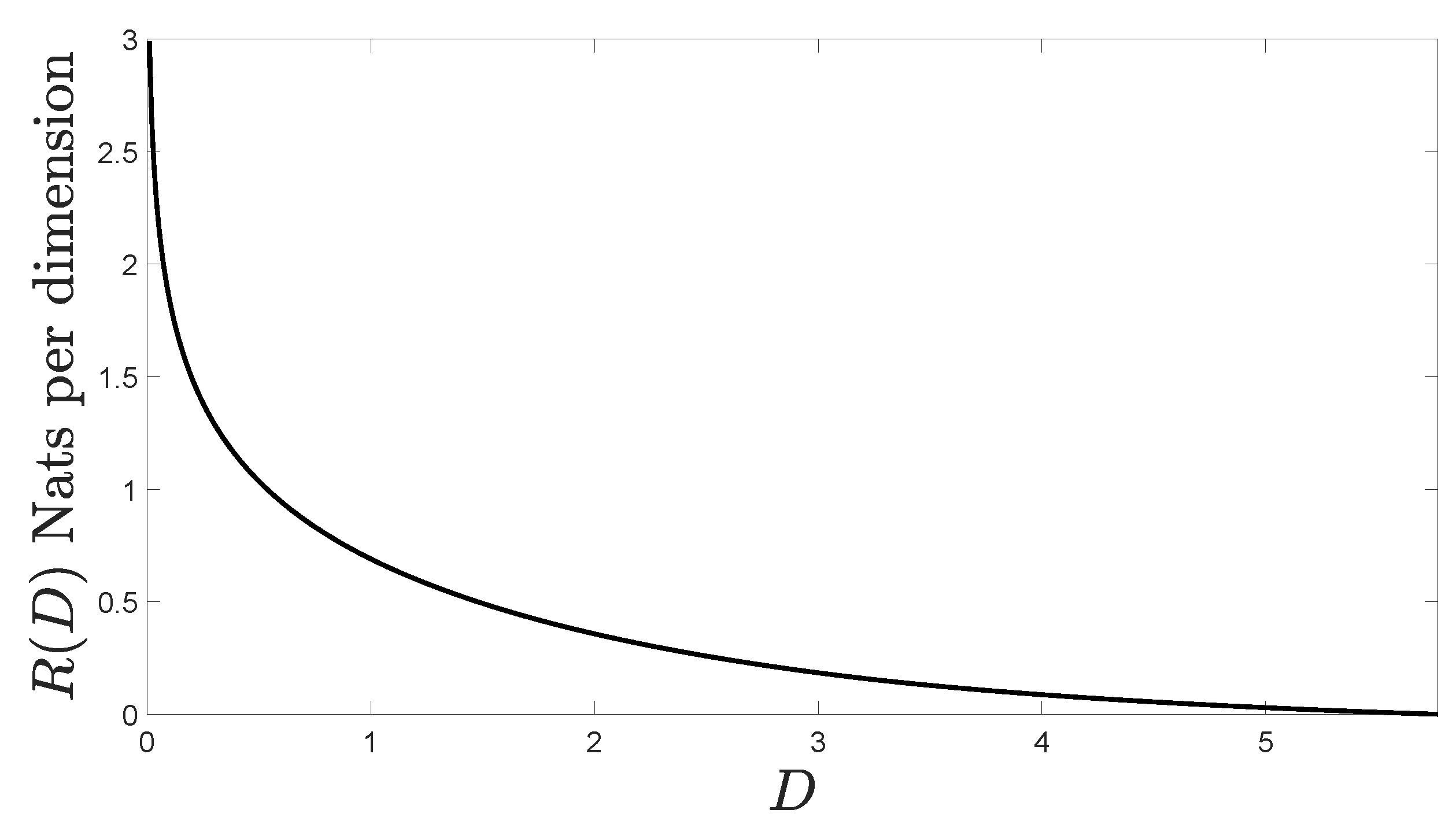
5. Numerical Example

We finish the paper with a numerical example where the RDF of a Gaussian AWSS vector process is computed. Specifically, we compute the RDF of the MA$\left(1\right)$ vector process considered in ([5], Example 2.1), by assuming that it is Gaussian.

Let $\{{\mathbf{x}}_n:n\in \mathbb{N}\}$ be as in Definition 3 with $N=2$,

$$G_{-1}=\left(\begin{array}{cc}-0.8& -0.7\\ 0.4& -0.6\end{array}\right),$$

${\mathrm{G}}_{-j}=0_{2\times 2}$ for all $j>1$, and:

$$\mathsf{\Lambda }=\left(\begin{array}{cc}4& 1\\ 1& 2\end{array}\right).$$

Assume that $\{{\mathbf{x}}_n:n\in \mathbb{N}\}$ is Gaussian. Figure 1 shows $R\left(D\right)$ with $D\in (0,5.77)$ that we have computed using Theorem 2.

Figure 1. Rate Distortion Function (RDF) of the Gaussian MA vector process considered.

References

- Hammerich, E. Waterfilling theorems for linear time-varying channels and related nonstationary sources. IEEE Trans. Inf. Theory 2016, 62, 6904–6916. [Google Scholar] [CrossRef]
- Kipnis, A.; Goldsmith, A.J.; Eldar, Y.C. The distortion rate function of cyclostationary Gaussian processes. IEEE Trans. Inf. Theory 2018, 64, 3810–3824. [Google Scholar] [CrossRef]
- Toms, W.; Berger, T. Information rates of stochastically driven dynamic systems. IEEE Trans. Inf. Theory 1971, 17, 113–114. [Google Scholar] [CrossRef]
- Kolmogorov, A.N. On the Shannon theory of information transmission in the case of continuous signals. IRE Trans. Inf. Theory 1956, 2, 102–108. [Google Scholar] [CrossRef]
- Reinsel, G.C. Elements of Multivariate Time Series Analysis; Springer: Berlin, Germany, 1993. [Google Scholar]
- Gray, R.M. Toeplitz and circulant matrices: A review. Found. Trends Commun. Inf. Theory 2006, 2, 155–239. [Google Scholar] [CrossRef]
- Ephraim, Y.; Lev-Ari, H.; Gray, R.M. Asymptotic minimum discrimination information measure for asymptotically weakly stationary processes. IEEE Trans. Inf. Theory 1988, 34, 1033–1040. [Google Scholar] [CrossRef]
- Gray, R.M. On the asymptotic eigenvalue distribution of Toeplitz matrices. IEEE Trans. Inf. Theory 1972, 18, 725–730. [Google Scholar] [CrossRef]
- Gutiérrez-Gutiérrez, J.; Crespo, P.M. Asymptotically equivalent sequences of matrices and Hermitian block Toeplitz matrices with continuous symbols: Applications to MIMO systems. IEEE Trans. Inf. Theory 2008, 54, 5671–5680. [Google Scholar] [CrossRef]
- Gutiérrez-Gutiérrez, J.; Crespo, P.M. Asymptotically equivalent sequences of matrices and multivariate ARMA processes. IEEE Trans. Inf. Theory 2011, 57, 5444–5454. [Google Scholar] [CrossRef]
- Gutiérrez-Gutiérrez, J.; Crespo, P.M. Block Toeplitz matrices: Asymptotic results and applications. Found. Trends Commun. Inf. Theory 2011, 8, 179–257. [Google Scholar] [CrossRef]
- Gutiérrez-Gutiérrez, J.; Crespo, P.M.; Zárraga-Rodríguez, M.; Hogstad, B.O. Asymptotically equivalent sequences of matrices and capacity of a discrete-time Gaussian MIMO channel with memory. IEEE Trans. Inf. Theory 2017, 63, 6000–6003. [Google Scholar] [CrossRef]
- Kafedziski, V. Rate distortion of stationary and nonstationary vector Gaussian sources. In Proceedings of the IEEE/SP 13th Workshop on Statistical Signal Processing, Bordeaux, France, 17–20 July 2005; IEEE: Piscataway, NJ, USA, 2005; pp. 1054–1059. [Google Scholar]
- Gazzah, H.; Regalia, P.A.; Delmas, J.P. Asymptotic eigenvalue distribution of block Toeplitz matrices and application to blind SIMO channel identification. IEEE Trans. Inf. Theory 2001, 47, 1243–1251. [Google Scholar] [CrossRef]
- Rudin, W. Principles of Mathematical Analysis; McGraw-Hill: New York, NY, USA, 1976. [Google Scholar]
- Gray, R.M. Information rates of autoregressive processes. IEEE Trans. Inf. Theory 1970, 16, 412–421. [Google Scholar] [CrossRef]
- Gallager, R.G. Information Theory and Reliable Communication; John Wiley & Sons: Hoboken, NJ, USA, 1968. [Google Scholar]
- Bhatia, R. Matrix Analysis; Springer: Berlin, Germany, 1997. [Google Scholar]
© 2018 by the authors. Licensee MDPI, Basel, Switzerland. This article is an open access article distributed under the terms and conditions of the Creative Commons Attribution (CC BY) license (http://creativecommons.org/licenses/by/4.0/).