Noise Enhancement for Weighted Sum of Type I and II Error Probabilities with Constraints

Abstract

In this paper, the noise-enhanced detection problem is investigated for the binary hypothesis-testing. The optimal additive noise is determined according to a criterion proposed by DeGroot and Schervish (2011), which aims to minimize the weighted sum of type I and II error probabilities under constraints on type I and II error probabilities. Based on a generic composite hypothesis-testing formulation, the optimal additive noise is obtained. The sufficient conditions are also deduced to verify whether the usage of the additive noise can or cannot improve the detectability of a given detector. In addition, some additional results are obtained according to the specificity of the binary hypothesis-testing, and an algorithm is developed for finding the corresponding optimal noise. Finally, numerical examples are given to verify the theoretical results and proofs of the main theorems are presented in the Appendix.

1. Introduction

In the binary hypothesis testing problem, there are usually a null hypothesis $H_0$ and an alternative hypothesis $H_1$, and the objective of testing is to be determine truthfulness of them based on the observation data and a decision rule. Due to the presence of noise, the decision result obviously cannot be absolutely correct. Generally, two erroneous decisions may occur in the signal detection: type I error that rejects a true null hypothesis and type II error that accepts a false null hypothesis [1].

In the classical statistical theory, the Neyman–Pearson criterion is usually applied to obtain a decision rule that minimizes the type II error probability $\beta$ with a constraint on the type I error probability $\alpha$. However, the minimum $\beta$ may not always correspond to the optimal decision result. For instance, in the example 1 of [2], a binary hypothesis testing is designed to determine the mean of a normal data: the mean equals to −1 under $H_0$ and equals to 1 under $H_1$. Under the constraint that the type I error probability is fixed to 0.05, the type II error probability is decreased from 0.0091 to 0.00000026 when the data size increases from 20 to 100, whereas the rejection region of the null hypothesis is changed from (0.1, +∞) to (−0.51, +∞). In such case, more information brings a worse decision result even a smaller type II error probability is achieved with the fixed type I error probability. Similarly, the decision rule that minimizes the type I error probability for a fixed type II error probability may not perform well. Therefore, it could not be appropriate to simply minimize one of the two error probabilities in practice. The ideal case is to develop a decision criterion that minimizes the two types of error probabilities simultaneously, but it is almost impossible in practical applications.

In order to obtain a better decision result to balance the type I and II error probabilities, DeGroot and Schervish [1] proposed a criterion to minimize a weighted sum of type I and II error probabilities, i.e., $\underset{\varphi }{\min }[c_1\cdot \alpha (\varphi )+c_2\cdot \beta (\varphi )]$, where $\varphi$ represents the decision rule, $c_1$ and $c_2$ are the weight coefficients corresponding to $\alpha$ and $\beta$, respectively, and $c_1,c_2>0$. Furthermore, DeGroot also provided the optimal decision procedure to minimize the weighted sum. The decision rule is given as follows. If $c_{1}f(x|H_0)<c_{2}f(x|H_1)$, the null hypothesis $H_0$ is rejected, where $f(x|H_0)$ and $f(x|H_1)$ are the respective probability density functions (pdfs) of the observation $\mathbf{x}$ under $H_0$ and $H_1$. If $c_{1}f(x|H_0)>c_{2}f(x|H_1)$, the alternative hypothesis $H_1$ is rejected. In addition, if $c_{1}f(x|H_0)=c_{2}f(x|H_1)$, the hypothesis $H_0$ can be either rejected or not. The optimal detector in this case is closely related to the distribution of the observation. This implies that once the distribution changes, the detector should be adjusted accordingly. But in the cases where the detector is fixed, this weighted sum rule cannot be directly applied. In such a case, finding an alternative method to minimize the weighted sum of type I and II error probabilities instead of changing the detector is important. Fortunately, the stochastic resonance (SR) theory provides a means to solve this problem.

The SR, first discovered by Benzi et al. [3] in 1981, is a phenomenon where noise plays a positive role in enhancing signal and system through a nonlinear system under certain conditions. The phenomenon of SR in the signal detection is also called noise-enhanced detection. Recent studies indicate that the system output performance can be improved significantly by adding noise to the system input or increasing the background noise level [4,5,6,7,8,9,10,11,12,13,14,15,16,17,18,19,20,21,22]. The improvements achieved via noise can be measured in the forms of increased signal-to-noise ratio (SNR) [7,8,9,10], mutual information (MI) [11,12] or detection probability [13,14,15,16], or in the form of decreased Bayes risk [17,18]. For example, the SNR gain of a parallel uncoupled array of bistable oscillators, operating in a mixture of sinusoidal signal and Gaussian white noise, is maximized via extra array noise [8]. In addition, due to the added array noise, the performance of a finite array closely approaches to an infinite array. In [11], the throughput MI of threshold neurons is increased by increasing the intensity of faint input noise. The optimal additive noise to maximize the detection probability with a constraint on false-alarm probability is studied in [13], and the sufficient conditions for improvability and non-improvability are deduced. In [17], the effects of additive independent noise on the performance of suboptimal detectors are investigated according to the restricted Bayes criterion, where the minimum noise modified Bayes risk is explored with certain constraints on the conditional risks. Inspired by this concept, it is reasonable to conjecture that a proper noise can decrease the weighted sum of type I and II error probabilities for a fixed detector.

In the absence of constraints, it is obvious that the additive noise that minimizes the weighted sum is a constant vector, whereas the corresponding type I or II error probability may exceed a certain value to cause a bad decision result. To avoid this problem, two constraints are enforced on type I and II error probabilities, respectively, to keep a balance. The aim of this work is to find the optimal additive noise that minimizes the weighted sum of type I and II error probabilities with the constraints on type I and II error probabilities for a fixed detector. Furthermore, the work can also be extended to some applications, such as the energy detection in sensor networks [23,24] and the independent Bernoulli trials [25]. The main contributions of this paper are summarized as follows:

• Formulation of the optimization problem for minimizing the noise modified weighted sum of type I and II error probabilities under the constraints on the two error probabilities is presented.
• Derivations of the optimal noise that minimizes the weighted sum and sufficient conditions for improvability and nonimprovability for a general composite hypothesis testing problem are provided.
• Analysis of the characteristics of the optimal additive noise that minimizes the weighted sum for a simple hypothesis testing problem is studied and the corresponding algorithm to solve the optimization problem is developed.
• Numerical results are presented to verify the theoretical results and to demonstrate the superior performance of the proposed detector.

The remainder of this paper is organized as follows: in Section 2, a noise modified composite hypothesis testing problem is formulated first for minimizing the weighted sum of type I and II error probabilities under different constraints. Then the sufficient conditions for improvability and nonimprovability are given and the optimal additive noise is derived. In Section 3, additional theoretical results are analyzed for a simple hypothesis testing problem. Finally, simulation results are shown in Section 4 and conclusions are made in Section 5.

Notation: Lower-case bold letters denote vectors, with ${\upsilon }_i$ denoting the i-th element of $\mathit{\upsilon }$; $\theta$ denotes the value of parameter $\mathrm{\Theta }$; $f_{\mathit{\upsilon }}(\mathit{\upsilon }|\theta )$ denotes the pdf of $\mathit{\upsilon }$ for a given parameter value $\mathrm{\Theta }=\theta$; ${\mathrm{\Omega }}_i$ denotes the set of all possible parameter values of $\mathrm{\Theta }$ under $H_i$; $\delta (\cdot )$ denotes the Dirac function; $\cap$, $\cup$ and $\varnothing$ denote intersection, union and null set, respectively; $\ast$, ${(\cdot )}^T$, ${\displaystyle \int }$, $E\{\cdot \}$, $\min$, $\max$ and $\arg$ denote convolution, transpose, integral, expectation, minimum, maximum and argument operators, respectively; $\inf \{\cdot \}$ and $\sup \{\cdot \}$ denote the infimum and supremum operators, respectively; ${\displaystyle \sum }$ means summation; $\nabla$ and $H$ denote the respective gradient and Hessian operators.

2. Noise Enhanced Composite Hypothesis Testing

2.1. Problem Formulation

Consider the following binary composite hypothesis testing problem:

$$\{\begin{array}{l}{H}_0:f_{\mathbf{x}}(\mathbf{x}|\theta ),\theta \in {\mathrm{\Omega }}_0\\ H_1:f_{\mathbf{x}}(\mathbf{x}|\theta ),\theta \in {\mathrm{\Omega }}_1\end{array}$$

(1)

where $\mathbf{x}\in {ℝ}^N$ is the observation vector, $H_0$ and $H_1$ are the null and the alternative hypothesizes, respectively, $\theta$ denotes the value of parameter $\mathrm{\Theta }$, $f_{\mathbf{x}}(\mathbf{x}|\theta )$ represents the pdf of $\mathbf{x}$ for a given parameter value $\mathrm{\Theta }=\theta$. The parameter $\mathrm{\Theta }$ has multiple possible values under each hypothesis and denote the pdf of any parameter value $\mathrm{\Theta }=\theta$ under $H_0$ and $H_1$ by ${\varpi }_0(\theta )$ and ${\varpi }_1(\theta )$. In addition, ${\mathrm{\Omega }}_0$ and ${\mathrm{\Omega }}_1$ denote the respective sets of all possible values of $\mathrm{\Theta }$ under $H_0$ and $H_1$. It is true that ${\mathrm{\Omega }}_0\cap {\mathrm{\Omega }}_1=\varnothing$ and the union of them forms the parameter space $\mathrm{\Omega }$, i.e., $\mathrm{\Omega }={\mathrm{\Omega }}_0\cup {\mathrm{\Omega }}_1$.

Without loss of generality, a decision rule (detector) is considered as:

$$\varphi (\mathbf{x})=\{\begin{array}{l}1,\mathbf{x}\in {\mathsf{\Gamma }}_1\\ 0,\mathbf{x}\in {\mathsf{\Gamma }}_0\end{array}$$

(2)

where ${\mathsf{\Gamma }}_0$ and ${\mathsf{\Gamma }}_1$ form the observation space $\mathsf{\Gamma }$. Actually, the detector chooses $H_1$ if $\mathbf{x}\in {\mathsf{\Gamma }}_1$, otherwise chooses $H_0$ if $\mathbf{x}\in {\mathsf{\Gamma }}_0$.

In order to investigate the performance of the detector achieved via an additive noise, a noise modified observation $\mathbf{y}$ is obtained by adding an independent additive noise $\mathbf{n}$ to the original observation $\mathbf{x}$, i.e., $\mathbf{y}=\mathbf{x}+\mathbf{n}$. For a given parameter value $\mathrm{\Theta }=\theta$, the pdf of $\mathbf{y}$ is calculated by the convolution of the pdfs of $\mathbf{x}$ and $\mathbf{n}$, given by:

$$f_{\mathbf{y}}(\mathbf{y}|\theta )=f_{\mathbf{x}}(\mathbf{x}|\theta )\ast p_{\mathbf{n}}(\mathbf{n})={\displaystyle {\int }_{{ℝ}^N}{p}_{\mathbf{n}}(\mathbf{n})f_{\mathbf{x}}(\mathbf{y}-\mathbf{n}|\theta )d\mathbf{n}}$$

(3)

where $p_{\mathbf{n}}(\mathbf{n})$ denotes the pdf of $\mathbf{n}$. For a fixed detector, the noise modified type I and II error probabilities of the detector for given parameter values now is expressed as:

$${\alpha }^{\mathbf{y}}(\varphi ;\theta )={\displaystyle {\int }_{\mathsf{\Gamma }}\varphi (\mathbf{y})f_{\mathbf{y}}(\mathbf{y}|\theta )d}\mathbf{y}={\displaystyle {\int }_{{\mathsf{\Gamma }}_1}{f}_{\mathbf{y}}(\mathbf{y}|\theta )d}\mathbf{y},\theta \in {\mathrm{\Omega }}_0$$

(4)

$${\beta }^{\mathbf{y}}(\varphi ;\theta )={\displaystyle {\int }_{\mathsf{\Gamma }}(1-\varphi (\mathbf{y}))f_{\mathbf{y}}(\mathbf{y}|\theta )d}\mathbf{y}={\displaystyle {\int }_{{\mathsf{\Gamma }}_0}{f}_{\mathbf{y}}(\mathbf{y}|\theta )d}\mathbf{y},\theta \in {\mathrm{\Omega }}_1$$

(5)

Correspondingly, the average noise modified type I and II error probabilities are calculated by:

$${\alpha }^{\mathbf{y}}(\varphi )={\displaystyle {\int }_{{\mathrm{\Omega }}_0}{\alpha }^{\mathbf{y}}(\varphi ;\theta ){\varpi }_0(\theta )d}\theta$$

(6)

$${\beta }^{\mathbf{y}}(\varphi )={\displaystyle {\int }_{{\mathrm{\Omega }}_1}{\beta }^{\mathbf{y}}(\varphi ;\theta ){\varpi }_1(\theta )d}\theta$$

(7)

From (6) and (7), the weighted sum of the two types of average error probabilities is obtained as:

$$\begin{array}{ll}E{r}^{\mathbf{y}}& =c_1\cdot {\alpha }^{\mathbf{y}}(\varphi )+c_2\cdot {\beta }^{\mathbf{y}}(\varphi )\\ & =c_1\cdot {\displaystyle {\int }_{{\mathrm{\Omega }}_0}{\alpha }^{\mathbf{y}}(\varphi ;\theta ){\varpi }_0(\theta )d}\theta +c_2\cdot {\displaystyle {\int }_{{\mathrm{\Omega }}_1}{\beta }^{\mathbf{y}}(\varphi ;\theta ){\varpi }_1(\theta )d}\theta \end{array}$$

(8)

where $c_1$ and $c_2$ are the weights assigned for the type I and II error probabilities, which can be predefined according to the actual situations. For example, if the prior probabilities are known, the value of $c_1$ and $c_2$ equal the prior probabilities corresponding to $H_0$ and $H_1$, respectively. Besides, the values of $c_1$ and $c_2$ can also be determined based on the expected decision results.

In this work, the aim is to find the optimal independent additive noise, which minimizes the weighted sum of the average error probabilities under the constraints on the maximum type I and II error probabilities for different parameter values. The optimization problem can be formulated as below:

$$p_{\mathbf{n}}^{opt}(\mathbf{n})=\arg \underset{p_{\mathbf{n}}(\mathbf{n})}{\min }E{r}^{\mathbf{y}}$$

(9)

subject to

$$\{\begin{array}{l}\underset{\theta \in {\mathrm{\Omega }}_0}{\max }{\alpha }^{\mathbf{y}}(\varphi ;\theta )\le {\alpha }_o\\ \underset{\theta \in {\mathrm{\Omega }}_1}{\max }{\beta }^{\mathbf{y}}(\varphi ;\theta )\le {\beta }_o\end{array}$$

(10)

where ${\alpha }_o$ and ${\beta }_o$ are the upper limits for the type I and II error probabilities, respectively.

In order to explicitly express the optimization problem described in (9) and (10), substituting (3) into (4) produces:

$$\begin{array}{ll}{\alpha }^{\mathbf{y}}(\varphi ;\theta )& ={\displaystyle {\int }_{{\mathsf{\Gamma }}_1}{\displaystyle {\int }_{{ℝ}^N}{p}_{\mathbf{n}}(\mathbf{n})f_{\mathbf{x}}(\mathbf{y}-\mathbf{n}|\theta )d\mathbf{n}}d}\mathbf{y}\\ & ={\displaystyle {\int }_{{ℝ}^N}{p}_{\mathbf{n}}(\mathbf{n}){\displaystyle {\int }_{{\mathsf{\Gamma }}_1}{f}_{\mathbf{x}}(\mathbf{y}-\mathbf{n}|\theta )d}\mathbf{y}d\mathbf{n}}\\ & ={\displaystyle {\int }_{{ℝ}^N}{p}_{\mathbf{n}}(\mathbf{n})A_{\theta }(\mathbf{n})d\mathbf{n}}\\ & =E\{A_{\theta }(\mathbf{n})\}\end{array},\theta \in {\mathrm{\Omega }}_0$$

(11)

where

$$A_{\theta }(\mathbf{n})={\displaystyle {\int }_{{\mathsf{\Gamma }}_1}{f}_{\mathbf{x}}(\mathbf{y}-\mathbf{n}|\theta )d}\mathbf{y}={\displaystyle {\int }_{\mathsf{\Gamma }}\varphi (\mathbf{y})f_{\mathbf{x}}(\mathbf{y}-\mathbf{n}|\theta )d}\mathbf{y},\theta \in {\mathrm{\Omega }}_0$$

(12)

It should be noted that $A_{\theta }(\mathbf{n})$ can be viewed as the type I error probability obtained by adding a constant vector $\mathbf{n}$ to $\mathbf{x}$ for $\theta \in {\mathrm{\Omega }}_0$. Therefore, ${\alpha }^{\mathbf{x}}(\varphi ;\theta )=A_{\theta }(0)={\displaystyle {\int }_{\mathsf{\Gamma }}\varphi (\mathbf{x})f_{\mathbf{x}}(\mathbf{x}|\theta )d}\mathbf{x}$ denotes the type I error probability for the original observation $\mathbf{x}$.

Similarly, ${\beta }^{\mathbf{y}}(\varphi ;\theta )$ in (5) can be expressed as:

$${\beta }^{\mathbf{y}}(\varphi ;\theta )=E\{B_{\theta }(\mathbf{n})\},\theta \in {\mathrm{\Omega }}_1$$

(13)

where

$$B_{\theta }(\mathbf{n})={\displaystyle {\int }_{{\mathsf{\Gamma }}_0}{f}_{\mathbf{x}}(\mathbf{y}-\mathbf{n}|\theta )d}\mathbf{y}={\displaystyle {\int }_{\mathsf{\Gamma }}(1-\varphi (\mathbf{y}))f_{\mathbf{x}}(\mathbf{y}-\mathbf{n}|\theta )d}\mathbf{y},\theta \in {\mathrm{\Omega }}_1$$

(14)

The $B_{\theta }(\mathbf{n})$ can be treated as the type II error probability obtained by adding a constant vector $\mathbf{n}$ to $\mathbf{x}$ for $\theta \in {\mathrm{\Omega }}_1$ and ${\beta }^{\mathbf{x}}(\varphi ;\theta )=B_{\theta }(0)={\displaystyle {\int }_{\mathsf{\Gamma }}(1-\varphi (\mathbf{x}))f_{\mathbf{x}}(\mathbf{x}|\theta )d}\mathbf{x}$ is the original type II error probability without adding noise for $\theta \in {\mathrm{\Omega }}_1$.

With (11) and (13), (8) becomes:

$$E{r}^{\mathbf{y}}={\displaystyle {\int }_{{ℝ}^N}{p}_{\mathbf{n}}(\mathbf{n})\left[c_1\cdot {\displaystyle {\int }_{{\mathrm{\Omega }}_0}{A}_{\theta }(\mathbf{n}){\varpi }_0(\theta )d}\theta +c_2\cdot {\displaystyle {\int }_{{\mathrm{\Omega }}_1}{B}_{\theta }(\mathbf{n}){\varpi }_1(\theta )d}\theta \right]d\mathbf{n}}=E\{Er(\mathbf{n})\}$$

(15)

where

$$Er(\mathbf{n})=c_1\cdot {\displaystyle {\int }_{{\mathrm{\Omega }}_0}{A}_{\theta }(\mathbf{n}){\varpi }_0(\theta )d}\theta +c_2\cdot {\displaystyle {\int }_{{\mathrm{\Omega }}_1}{B}_{\theta }(\mathbf{n}){\varpi }_1(\theta )d}\theta$$

(16)

Accordingly, $Er(\mathbf{n})$ is the weighted sum of two types of average error probabilities achieved by adding a constant vector $\mathbf{n}$ to the original observation $\mathbf{x}$. Naturally, $E{r}^{\mathbf{x}}=Er(0)$ denotes the weighted sum of type I and II average error probabilities for the original observation $\mathbf{x}$.

Combined (11), (13) and (15), the optimization problem in (9) and (10) now is:

$$p_{\mathbf{n}}^{opt}(\mathbf{n})=\arg \underset{p_{\mathbf{n}}(\mathbf{n})}{\min }E\{Er(\mathbf{n})\}$$

(17)

subject to

$$\{\begin{array}{l}\underset{\theta \in {\mathrm{\Omega }}_0}{\max }E\{A_{\theta }(\mathbf{n})\}\le {\alpha }_o\\ \underset{\theta \in {\mathrm{\Omega }}_1}{\max }E\{B_{\theta }(\mathbf{n})\}\le {\beta }_o\end{array}$$

(18)

2.2. Sufficient Conditions for Improvability and Non-improvability

In practice, the solution of the optimization problem in (17) and (18) requires a research over all possible noises and this procedure is complicated. Therefore, it is worthwhile to determine whether the detector can or cannot be improved by adding additive noise in advance. From (17) and (18), a detector is considered to be improvable if there exists one noise $\mathbf{n}$ that satisfies $E\{Er(\mathbf{n})\}<E{r}^{\mathbf{x}}=Er(0)$, $\underset{\theta \in {\mathrm{\Omega }}_0}{\max }E\{A_{\theta }(\mathbf{n})\}\le {\alpha }_o$ and $\underset{\theta \in {\mathrm{\Omega }}_0}{\max }E\{B_{\theta }(\mathbf{n})\}\le {\beta }_o$ simultaneously; otherwise, the detector is considered to be non-improvable.

The sufficient conditions for non-improvability can be obtained according to the characteristics of $A_{\theta }(\mathbf{n})$, $B_{\theta }(\mathbf{n})$ and $Er(\mathbf{n})$, which are provided in Theorem 1.

Theorem 1.

If there exists ${\theta }^{*}\in {\mathrm{\Omega }}_0$ (${\theta }^{*}\in {\mathrm{\Omega }}_1$) such that $A_{{\theta }^{*}}(\mathbf{n})\le {\alpha }_o$ ($B_{{\theta }^{*}}(\mathbf{n})\le {\beta }_o$) implies $Er(\mathbf{n})\ge Er(0)$ for any $\mathbf{n}\in P_{\mathbf{n}}$, where $P_{\mathbf{n}}$ represents the convex set of all possible additive noises, and if $A_{{\theta }^{*}}(\mathbf{n})$ ($B_{{\theta }^{*}}(\mathbf{n})$ ) and $Er(\mathbf{n})$ are convex functions over $P_{\mathbf{n}}$, then the detector is non-improvable.

The proof is provided in Appendix A.

Under the conditions in Theorem 1, the detector cannot be improved and it is unnecessary to solve the optimization problem in (17) and (18). In other words, if the conditions in Theorem 1 are satisfied, the three inequities $E{r}^{\mathbf{y}}\ge E{r}^{\mathbf{x}}$, $\underset{\theta \in {\mathrm{\Omega }}_0}{\max }E\{A_{\theta }(\mathbf{n})\}\le {\alpha }_o$ and $\underset{\theta \in {\mathrm{\Omega }}_1}{\max }E\{B_{\theta }(\mathbf{n})\}\le {\beta }_o$ cannot be achieved simultaneously by adding any additive noise. In addition, even if the conditions in Theorem 1 are not satisfied, the detector can also be non-improvable. This implies the sufficient conditions for improvability need to be addressed.

The sufficient conditions for improvability are discussed now. Suppose that $A_{\theta }(\mathbf{x})$ ($\forall \theta \in {\mathrm{\Omega }}_0$), $B_{\theta }(\mathbf{x})$ ($\forall \theta \in {\mathrm{\Omega }}_1$) and $Er(\mathbf{x})$ are second-order continuously differentiable around $\mathbf{x}=0$. In order to facilitate the subsequent analysis, six auxiliary functions are predefined as follows based on the first and second partial derivatives of $A_{\theta }(\mathbf{x})$, $B_{\theta }(\mathbf{x})$ and $Er(\mathbf{x})$ with respect to the elements of $\mathbf{x}$. The first three auxiliary functions $a_{\theta }^{(1)}(\mathbf{x},\mathbf{g})$, $b_{\theta }^{(1)}(\mathbf{x},\mathbf{g})$ and $e{r}^{(1)}(\mathbf{x},\mathbf{g})$ are defined as the weight sums of the first partial derivatives of $A_{\theta }(\mathbf{x})$, $B_{\theta }(\mathbf{x})$ and $Er(\mathbf{x})$, respectively, based on the coefficient vector $\mathbf{g}$. Specifically:

$$a_{\theta }^{(1)}(\mathbf{x},\mathbf{g})\triangleq {\displaystyle \sum _{i=1}^N{g}_i\frac{\partial A_{\theta }(\mathbf{x})}{\partial {\mathbf{x}}_i}={\mathbf{g}}^T\nabla A_{\theta }(\mathbf{x})},\theta \in {\mathrm{\Omega }}_0$$

(19)

$$b_{\theta }^{(1)}(\mathbf{x},\mathbf{g})\triangleq {\displaystyle \sum _{i=1}^N{g}_i\frac{\partial B_{\theta }(\mathbf{x})}{\partial {\mathbf{x}}_i}}={\mathbf{g}}^T\nabla B_{\theta }(\mathbf{x}),\theta \in {\mathrm{\Omega }}_1$$

(20)

$$e{r}^{(1)}(\mathbf{x},\mathbf{g})\triangleq {\displaystyle \sum _{i=1}^N{g}_i\frac{\partial Er(\mathbf{x})}{\partial {\mathbf{x}}_i}}={\mathbf{g}}^T\nabla Er(\mathbf{x})$$

(21)

where $\mathbf{g}$ is a $N$-dimensional column vector, ${\mathbf{g}}^T$is the transposition of $\mathbf{g}$, ${\mathbf{x}}_i$ and ${\mathbf{g}}_i$ are the i-th elements of $\mathbf{x}$ and $\mathbf{g}$, respectively. In addition, $\nabla$ denotes the gradient operator, thereby $\nabla A_{\theta }(\mathbf{x})$ ($\nabla B_{\theta }(\mathbf{x})$,$\nabla Er(\mathbf{x})$) is a $N$-dimensional column vector with i-th element $\partial A_{\theta }(\mathbf{x})/\partial {\mathbf{x}}_i$ ($\partial B_{\theta }(\mathbf{x})/\partial {\mathbf{x}}_i$, $\partial E_r(\mathbf{x})/\partial {\mathbf{x}}_i$), $i=1,\dots ,N$. The last three auxiliary functions $a_{\theta }^{(2)}(\mathbf{x},\mathbf{g})$, $b_{\theta }^{(2)}(\mathbf{x},\mathbf{g})$ and $e{r}^{(2)}(\mathbf{x},\mathbf{g})$ are defined as the weight sums of the second partial derivatives of $A_{\theta }(\mathbf{x})$, $B_{\theta }(\mathbf{x})$ and $Er(\mathbf{x})$ based on the $N\times N$ coefficient matrix $\mathbf{g}{\mathbf{g}}^T$, i.e.,

$$a_{\theta }^{(2)}(\mathbf{x},\mathbf{g})\triangleq {\displaystyle \sum _{j=1}^N{\displaystyle \sum _{i=1}^N{g}_j{g}_i\frac{{\partial }^2{A}_{\theta }(\mathbf{x})}{(\partial {\mathbf{x}}_j\partial {\mathbf{x}}_i)}={\mathbf{g}}^{T}H(A_{\theta }(\mathbf{x}))\mathbf{g}}},\theta \in {\mathrm{\Omega }}_0$$

(22)

$$b_{\theta }^{(2)}(\mathbf{x},\mathbf{g})\triangleq {\displaystyle \sum _{j=1}^N{\displaystyle \sum _{i=1}^N{g}_j{g}_i\frac{{\partial }^2{B}_{\theta }(\mathbf{x})}{(\partial {\mathbf{x}}_j\partial {\mathbf{x}}_i)}}}={\mathbf{g}}^{T}H(B_{\theta }(\mathbf{x}))\mathbf{g},\theta \in {\mathrm{\Omega }}_1$$

(23)

$$e{r}^{(2)}(\mathbf{x},\mathbf{g})\triangleq {\displaystyle \sum _{j=1}^N{\displaystyle \sum _{i=1}^N{g}_j{g}_i\frac{{\partial }^{2}Er(\mathbf{x})}{(\partial {\mathbf{x}}_j\partial {\mathbf{x}}_i)}}}={\mathbf{g}}^{T}H(Er(\mathbf{x}))\mathbf{g}$$

(24)

where $H$ denote the Hessian operator, $H(A_{\theta }(\mathbf{x}))$ ($H(B_{\theta }(\mathbf{x}))$,$H(Er(\mathbf{x}))$) is a $N\times N$ matrix with its $(j,i)$-th element denoted by ${\partial }^2{A}_{\theta }(\mathbf{x})/(\partial {\mathbf{x}}_j\partial {\mathbf{x}}_i)$ (${\partial }^2{B}_{\theta }(\mathbf{x})/(\partial {\mathbf{x}}_j\partial {\mathbf{x}}_i)$,${\partial }^{2}Er(\mathbf{x})/(\partial {\mathbf{x}}_j\partial {\mathbf{x}}_i)$), where $i,j=1,\dots ,N$.

Based on the definitions in (19)–(24), Theorem 2 presents the sufficient conditions for improvability.

Theorem 2.

Suppose that ${\mathrm{\Lambda }}_0$ and ${\mathrm{\Lambda }}_1$ are the sets of all possible values of $\theta$ that maximize $A_{\theta }(0)$ and $B_{\theta }(0)$, respectively, ${\alpha }_o=\underset{\theta \in {\mathrm{\Omega }}_0}{\max }{A}_{\theta }(0)$ and ${\beta }_o=\underset{\theta \in {\mathrm{\Omega }}_1}{\max }{B}_{\theta }(0)$. The detector is improvable, if there exists a $N$-dimensional column vector $\mathbf{g}$ that satisfies one of the following conditions for all ${\theta }_0\in {\mathrm{\Lambda }}_0$ and ${\theta }_1\in {\mathrm{\Lambda }}_1$ :

(1) 

$e{r}^{(1)}(\mathbf{x},\mathbf{g}){|}_{\mathbf{x}=0}<0$, $a_{{\theta }_0}^{(1)}(\mathbf{x},\mathbf{g}){|}_{\mathbf{x}=0}<0$, $b_{{\theta }_1}^{(1)}(\mathbf{x},\mathbf{g}){|}_{\mathbf{x}=0}<0$;

(2) 

$e{r}^{(1)}(\mathbf{x},\mathbf{g}){|}_{\mathbf{x}=0}>0$, $a_{{\theta }_0}^{(1)}(\mathbf{x},\mathbf{g}){|}_{\mathbf{x}=0}>0$, $b_{{\theta }_1}^{(1)}(\mathbf{x},\mathbf{g}){|}_{\mathbf{x}=0}>0$;

(3) 

$e{r}^{(2)}(\mathbf{x},\mathbf{g}){|}_{\mathbf{x}=0}<0$, $a_{{\theta }_0}^{(2)}(\mathbf{x},\mathbf{g}){|}_{\mathbf{x}=0}<0$, $b_{{\theta }_1}^{(2)}(\mathbf{x},\mathbf{g}){|}_{\mathbf{x}=0}<0$.

The proof is presented in Appendix B.

Theorem 2 indicates that under the condition (1), (2) or (3), there always exist noises that decrease the weighted sum of average error probabilities under the constraints on the type I and II error probabilities. In addition, alternative sufficient conditions for improvability can be obtained by defining the following two functions, and they are:

$$I(t)=\inf \{Er(\mathbf{n})|\underset{\theta \in {\mathrm{\Omega }}_0}{\max }{A}_{\theta }(\mathbf{n})=t,\mathbf{n}\in {ℝ}^N\}$$

(25)

$$S(t)=\sup \{\underset{\theta \in {\mathrm{\Omega }}_1}{\max }{B}_{\theta }(\mathbf{n})|\underset{\theta \in {\mathrm{\Omega }}_0}{\max }{A}_{\theta }(\mathbf{n})=t,\mathbf{n}\in {ℝ}^N\}$$

(26)

where $I(t)$ and $S(t)$ are the minimum weighted sum of two types of average error probabilities and the maximum type II error probability for a given maximum type I error probability obtained via adding a constant vector, respectively. If there is a $t_0\le {\alpha }_o$ such that $I(t_0)\le Er(0)$ and $S(0)\le {\beta }_o$, the detector is improvable. More specifically, there exists a constant vector ${\mathbf{n}}_0$ that satisfies $\underset{\theta \in {\mathrm{\Omega }}_0}{\max }{A}_{\theta }({\mathbf{n}}_0)=t_0\le {\alpha }_o$, $Er({\mathbf{n}}_0)\le Er(0)$ and $\underset{\theta \in {\mathrm{\Omega }}_0}{\max }{B}_{\theta }({\mathbf{n}}_0)\le {\beta }_o$ simultaneously. However, in most cases, the solution of the optimization problem in (17) and (18) is not a constant vector. A more practical sufficient condition for improvability is shown in Theorem 3.

Theorem 3.

Let $\tilde{\alpha }=\underset{\theta \in {\mathrm{\Omega }}_0}{\max }{\alpha }^{\mathbf{x}}(\varphi ;\theta )$ and $\tilde{\beta }=\underset{\theta \in {\mathrm{\Omega }}_1}{\max }{\beta }^{\mathbf{x}}(\varphi ;\theta )$ be the respective maximum type I and II error probabilities without adding any noise, and suppose that $\tilde{\alpha }\le {\alpha }_o$, $\tilde{\beta }\le {\beta }_o$ and $S(\tilde{\alpha })=\tilde{\beta }$. If $I(t)$ and $S(t)$ are second-order continuously differentiable around $t=\tilde{\alpha }$, and $I^{″}(\tilde{\alpha })<0$ and $S^{″}(\tilde{\alpha })<0$ hold at the same time, then the detector is improvable.

The proof is given in Appendix C.

Additionally, the following functions $J(\epsilon )$ and $G(\epsilon )$ are defined:

$$J(\epsilon )=\inf \{Er(\mathbf{n})|\underset{\theta \in {\mathrm{\Omega }}_1}{\max }{B}_{\theta }(\mathbf{n})=\epsilon ,\mathbf{n}\in {ℝ}^N\}$$

(27)

$$G(\epsilon )=\sup \{\underset{\theta \in {\mathrm{\Omega }}_0}{\max }{A}_{\theta }(\mathbf{n})|\underset{\theta \in {\mathrm{\Omega }}_1}{\max }{B}_{\theta }(\mathbf{n})=\epsilon ,\mathbf{n}\in {ℝ}^N\}$$

(28)

A similar conclusion to the Theorem 3 can be made as well, provided in Corollary 1.

Corollary 1.

The detector is improvable, if $J^{″}(\tilde{\beta })\le 0$ and $G^{″}(\tilde{\beta })\le 0$ hold, where $J(\epsilon )$ and $G(\epsilon )$ are second-order continuously differentiable around $\epsilon =\tilde{\beta }$, and $G(\tilde{\beta })=\tilde{\alpha }$.

The proof is similar to that of Theorem 3 and it is omitted here.

2.3. Optimal Additive Noise

In general, it is difficult to solve the optimization problem in (17) and (18) directly, because the solution is obtained based on the search over all possible additive noises. Hence, in order to reduce the computational complexity, one can utilize Parzen window density estimation to obtain an approximate solution. Actually, the pdf of the optimal additive noise can be approximated by:

$$p_{\mathbf{n}}(\mathbf{n})={\displaystyle \sum _{l=1}^L{\eta }_l{\vartheta }_l(\mathbf{n})}$$

(29)

where ${\eta }_l\ge 0$ and ${\displaystyle {\sum }_{l=1}^L{\eta }_l}=1$, while ${\vartheta }_l(\cdot )$ represents the window function that satisfies ${\vartheta }_l(\mathbf{x})\ge 0$ for any $\mathbf{x}$ and ${\displaystyle \int {\vartheta }_l(\mathbf{x})d\mathbf{x}=0}$ for $l=1,\dots ,L$. The window function can be a cosine window, rectangular window, or Gauss window function. With (29), the optimization problem is simplified to obtain the parameter values corresponding to each window function. In such cases, global optimization algorithms can be applied such as Particle swarm optimization (PSO), Ant colony algorithm (ACA), and Genetic algorithm (GA) [26,27,28].

If the numbers of parameter values in ${\mathrm{\Omega }}_0$ and ${\mathrm{\Omega }}_1$ are finite, the optimal additive noise for (17) and (18) is a randomization of no more than $M+K$ constant vectors. In this case, ${\mathrm{\Omega }}_0$ and ${\mathrm{\Omega }}_1$ can be expressed by ${\mathrm{\Omega }}_0=\{{\theta }_{01},{\theta }_{02},\dots ,{\theta }_{0M}\}$ and ${\mathrm{\Omega }}_1=\{{\theta }_{11},{\theta }_{12},\dots ,{\theta }_{1K}\}$, where $M$ and $K$ are finite positive integers. The Theorem 4 states this claim.

Theorem 4.

Suppose that each component in the optimal additive noise is finite, namely $n_i\in [a_i,b_i]$ for $i=1,\dots ,N$, where $a_i$ and $b_i$ are two finite values. If $A_{{\theta }_{0i}}(\cdot )$ and $B_{{\theta }_{1i}}(\cdot )$ are continuous functions, the pdf of the optimal additive noise for the optimization problem in (17) and (18) can be expressed as:

$$p_{\mathbf{n}}(\mathbf{n})={\displaystyle \sum _{l=1}^{M+K}{\eta }_l\delta (\mathbf{n}-{\mathbf{n}}_l)}$$

(30)

where ${\eta }_l\ge 0$ and ${\displaystyle {\sum }_{l=1}^{M+K}{\eta }_l}=1$.

The proof is similar to that of Theorem 4 in [17] and Theorem 3 in [13], and omitted here. In some special cases, the optimal additive can be solved directly based on the characteristics of $I(t)$ ($H(\epsilon )$). For example, let $E{r}_{\min }=\underset{t}{\min }I(t)=I(t_m)$ ($E{r}_{\min }=\underset{\epsilon }{\min }H(\epsilon )=I({\epsilon }_m)$) and $\underset{\theta \in {\mathrm{\Omega }}_0}{\max }{A}_{\theta }({\mathbf{n}}_m)=t_m$ ($\underset{\theta \in {\mathrm{\Omega }}_1}{\max }{B}_{\theta }({\mathbf{n}}_m)={\epsilon }_m$). If $t_m\le {\alpha }_o$ (${\epsilon }_m\le {\beta }_o$) and $\underset{\theta \in {\mathrm{\Omega }}_1}{\max }{B}_{\theta }({\mathbf{n}}_m)\le {\beta }_o$ ($\underset{\theta \in {\mathrm{\Omega }}_0}{\max }{A}_{\theta }({\mathbf{n}}_m)\le$${\alpha }_o$), the optimal additive noise is a constant vector with pdf of $p_{\mathbf{n}}(\mathbf{n})=\delta (\mathbf{n}-{\mathbf{n}}_m)$. In addition, equality of $\underset{\theta \in {\mathrm{\Omega }}_0}{\max }E\{A_{\theta }(\mathbf{n})\}={\alpha }_o$ ($\underset{\theta \in {\mathrm{\Omega }}_1}{\max }E\{B_{\theta }(\mathbf{n})\}={\beta }_o$) holds if $t_m>{\alpha }_o$ (${\epsilon }_m>{\beta }_o$).

3. Noise Enhanced Simple Hypothesis Testing

In this section, the noise enhanced binary simple hypothesis testing problem is considered, which is a special case of the optimization problem in (9) and (10). Therefore, the conclusions obtained in Section 2 are also applicable in this section. Furthermore, due to the specificity of simple binary hypothesis testing problem, some additional results are also obtained.

3.1. Problem Formulation

When ${\mathrm{\Omega }}_i=\{{\theta }_i\}$, $i=0,1$, the composite binary hypothesis testing problem described in (1) is simplified to a simple binary hypothesis testing problem. In this case, the probability of ${\theta }_i$ under $H_i$ equals to 1, i.e., ${\varpi }_i(\theta )=1$ for $i=0,1$. Therefore, the corresponding noise modified type I and II error probabilities is rewritten as:

$${\alpha }^{\mathbf{y}}(\varphi )={\alpha }^{\mathbf{y}}(\varphi ;{\theta }_0)={\displaystyle {\int }_{{ℝ}^N}{p}_{\mathbf{n}}(\mathbf{n}){\displaystyle {\int }_{{\mathsf{\Gamma }}_1}{f}_0(\mathbf{y}-\mathbf{n})d}\mathbf{y}d\mathbf{n}}=E\{A_0(\mathbf{n})\}$$

(31)

$${\beta }^{\mathbf{y}}(\varphi )={\beta }^{\mathbf{y}}(\varphi ;{\theta }_1)={\displaystyle {\int }_{{ℝ}^N}{p}_{\mathbf{n}}(\mathbf{n}){\displaystyle {\int }_{{\mathsf{\Gamma }}_0}{f}_1(\mathbf{y}-\mathbf{n})d}\mathbf{y}d\mathbf{n}}=E\{B_1(\mathbf{n})\}$$

(32)

where $f_0(\cdot )$ and $f_1(\cdot )$ represent the pdfs of $\mathbf{x}$ under $H_0$ and $H_1$, respectively, and $A_0(\mathbf{n})$ and $B_1(\mathbf{n})$ are:

$$A_0(\mathbf{n})={\displaystyle {\int }_{{\mathsf{\Gamma }}_1}{f}_0(\mathbf{y}-\mathbf{n})d}\mathbf{y}$$

(33)

$$B_1(\mathbf{n})={\displaystyle {\int }_{{\mathsf{\Gamma }}_0}{f}_1(\mathbf{y}-\mathbf{n})d}\mathbf{y}$$

(34)

Correspondingly, the weighted sum of noise modified type I and II error probabilities is calculated by:

$$\begin{array}{ll}E{r}^{\mathbf{y}}& =c_1{\alpha }^{\mathbf{y}}(\varphi )+c_2{\beta }^{\mathbf{y}}(\varphi )=c_{1}E\{A_0(\mathbf{n})\}+c_{2}E\{B_1(\mathbf{n})\}\\ & ={\displaystyle {\int }_{{ℝ}^N}{p}_{\mathbf{n}}(\mathbf{n})(c_1{A}_0(\mathbf{n})+c_2{B}_1(\mathbf{n}))d\mathbf{n}}\\ & =E\{Er(\mathbf{n})\}\end{array}$$

(35)

where

$$Er(\mathbf{n})=c_1{A}_0(\mathbf{n})+c_2{B}_1(\mathbf{n})$$

(36)

As a result, the optimization problem in (9) and (10) becomes:

$$p_{\mathbf{n}}^{opt}(\mathbf{n})=\arg \underset{p_{\mathbf{n}}(\mathbf{n})}{\min }E\{Er(\mathbf{n})\}$$

(37)

subject to

$$\{\begin{array}{l}E\{A_0(\mathbf{n})\}\le {\alpha }_o\\ E\{B_1(\mathbf{n})\}\le {\beta }_o\end{array}$$

(38)

Based on the definitions in (33) and (34), $A_0(\mathbf{n})$ and $B_1(\mathbf{n})$ are viewed as the noise modified type I and II error probabilities obtained by adding a constant vector noise. Furthermore, $A_0(0)$ and $B_1(0)$ are the original type I and II error probabilities, respectively.

3.2. Algorithm for the Optimal Additive Noise

According to the Theorem 4 in Section 2.3, the optimal additive noise for the optimization problem in (37) and (38) is a randomization of most two constant vectors with the pdf $p_{\mathbf{n}}^{opt}(\mathbf{n})=\eta \delta (\mathbf{n}-{\mathbf{n}}_1)+(1-\eta )\delta (\mathbf{n}-{\mathbf{n}}_2)$. In order to find the values of $\eta$, ${\mathbf{n}}_1$ and ${\mathbf{n}}_2$, we first divide each constant vector $\mathbf{n}$ into four disjoint sets according to the relationships of $A_0(\mathbf{n})$ and ${\alpha }_o$, $B_1(\mathbf{n})$ and ${\beta }_o$. To be specific, the four disjoint sets are $Q_1=\{\mathbf{n}|A_0(\mathbf{n})\le {\alpha }_o,B_1(\mathbf{n})\le {\beta }_o\}$, $Q_2=\{\mathbf{n}|A_0(\mathbf{n})\le {\alpha }_o,B_1(\mathbf{n})>{\beta }_o\}$, $Q_3=\{\mathbf{n}|A_0(\mathbf{n})>{\alpha }_o,B_1(\mathbf{n})\le {\beta }_o\}$, and $Q_4=\{\mathbf{n}|A_0(\mathbf{n})>{\alpha }_o,B_1(\mathbf{n})>{\beta }_o\}$. Then, we calculate the minimum $Er(\mathbf{n})$, the corresponding set of all possible values of $\mathbf{n}$ is denoted by $Q_e=\{\mathbf{n}|\mathbf{n}=\arg \underset{\mathbf{n}}{\min }Er(\mathbf{n})\}$. It should be noted that $\mathbf{n}\in Q_e$ is the optimal additive noise that minimizes the weighted sum without constraints.

It is obvious that $Q_1$, $Q_2$ and $Q_3$ do not exist if all the elements of $Q_e$ belong to $Q_4$. In other words, if $Q_e\subset Q_4$, there is no additive noise that satisfies $E\{Er(\mathbf{n})\}<Er(0)$ under the constraints of $E\{A_0(\mathbf{n})\}\le {\alpha }_o$ and $E\{B_1(\mathbf{n})\}\le {\beta }_o$. Therefore, if the detector is improvable, the elements of $Q_e$ must come from $Q_1$, $Q_2$ and/or $Q_3$. Theorem 5 is now provided to find the values of $\eta$, ${\mathbf{n}}_1$ and ${\mathbf{n}}_2$.

Theorem 5.

Let ${\eta }_1=\frac{{\alpha }_o-A_0({\mathbf{n}}_2)}{A_0({\mathbf{n}}_1)-A_0({\mathbf{n}}_2)}$ and ${\eta }_2=\frac{{\beta }_o-B_1({\mathbf{n}}_2)}{B_1({\mathbf{n}}_1)-B_1({\mathbf{n}}_2)}$.

(1) 

If $Q_e\cap Q_1\ne \varnothing$, then $\eta =1$ and ${\mathbf{n}}_1\in Q_e\cap Q_1$ such that $E{r}_{opt}^{\mathbf{y}}=Er({\mathbf{n}}_1)=\underset{\mathbf{n}}{\min }Er(\mathbf{n})$.

(2) 

If $Q_e\cap Q_2\ne \varnothing$ and $Q_e\cap Q_3\ne \varnothing$ are true, then we have ${\mathbf{n}}_1\in Q_e\cap Q_2$, ${\mathbf{n}}_2\in Q_e\cap Q_3$, ${\eta }_1\le \eta \le {\eta }_2$, and $E{r}_{opt}^{\mathbf{y}}=\underset{\mathbf{n}}{\min }Er(\mathbf{n})$.

(3) 

If $Q_e\subset Q_2$, then $E{r}_{opt}^{\mathbf{y}}$ is obtained when $\eta ={\eta }_2$, and the corresponding $E\{A_0(\mathbf{n})\}$ achieves the minimum and $E\{B_1(\mathbf{n})\}={\beta }_o$.

(4) 

If $Q_e\subset Q_3$, then $E{r}_{opt}^{\mathbf{y}}$ is achieved when $\eta ={\eta }_1$, and the corresponding $E\{A_0(\mathbf{n})\}={\alpha }_o$ and $E\{B_1(\mathbf{n})\}$ reaches the minimum.

The corresponding proofs are provided in Appendix D.

From (3) and (4) in Theorem 5, under the constraints on $E\{A_0(\mathbf{n})\}\le {\alpha }_o$ and $E\{B_1(\mathbf{n})\}\le {\beta }_o$, the solution of the optimization problem in (37) and (38) is identical with the additive noise that minimizes $E\{A_0(\mathbf{n})\}$ ($E\{B_1(\mathbf{n})\}$) when $Q_e\subset Q_2$ ($Q_e\subset Q_3$). In such cases, the optimal solution can be obtained easily by referring the algorithm provided in [14].

4. Numerical Results

In this section, a binary hypothesis testing problem is studied to verify the theoretical analysis, and it is:

$$\{\begin{array}{l}{H}_0:x=v\\ H_1:x=\mathrm{\Theta }+v\end{array}$$

(39)

where $x\in ℝ$ is an observation, $\mathrm{\Theta }$ is a constant or random variable, and $v$ is the background noise with pdf $p_v(\cdot )$. From (39), the pdf of $x$ under $H_0$ is $f_0(x)=p_v(x)$, and the pdf of $x$ under $H_1$ for a given parameter value $\mathrm{\Theta }=\theta$ is denoted by $f_{\theta }(x)=p_v(\cdot )\ast p_{\theta }(\cdot )$, where $p_{\theta }(\cdot )$ represents the pdf of $\mathrm{\Theta }=\theta$. A noise modified observation $y$ is obtained via adding an additive independent noise $n$ to the observation $x$, i.e., $y=x+n$. If the additive noise $n$ is a constant vector, the pdf of $y$ under $H_0$ is calculated as $f_0(y)=f_0(x-n)$, and the pdf of $y$ under $H_1$ for $\mathrm{\Theta }=\theta$ is $f_{\theta }(y)=f_{\theta }(x-n)$. In addition, a linear- quadratic detector is utilized here, given by:

$$T(y)=d_0{y}^2+d_{1}y+d_2\stackrel{H_1}{\underset{H_0}{\underset{<}{>}}}\gamma$$

(40)

where $d_0$, $d_1$ and $d_2$ are detector parameters, and $\gamma$ denotes the detection threshold. In the numerical examples, ${\alpha }_o={\alpha }^x$ and ${\beta }_o={\beta }^x$, where ${\alpha }^x$ and ${\beta }^x$ are the original type I and II error probabilities, respectively.

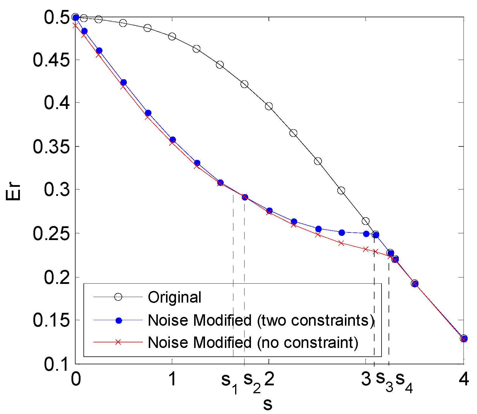
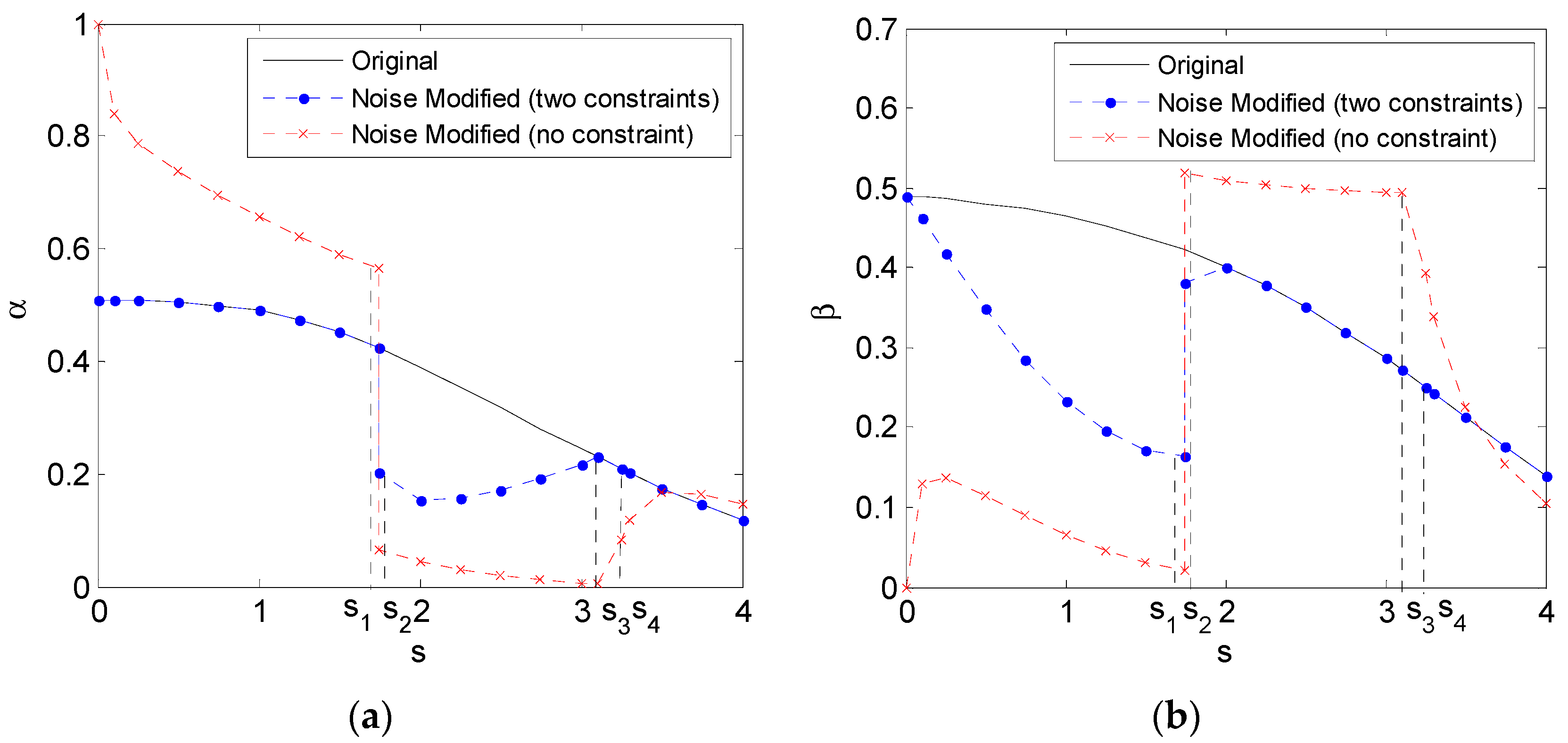
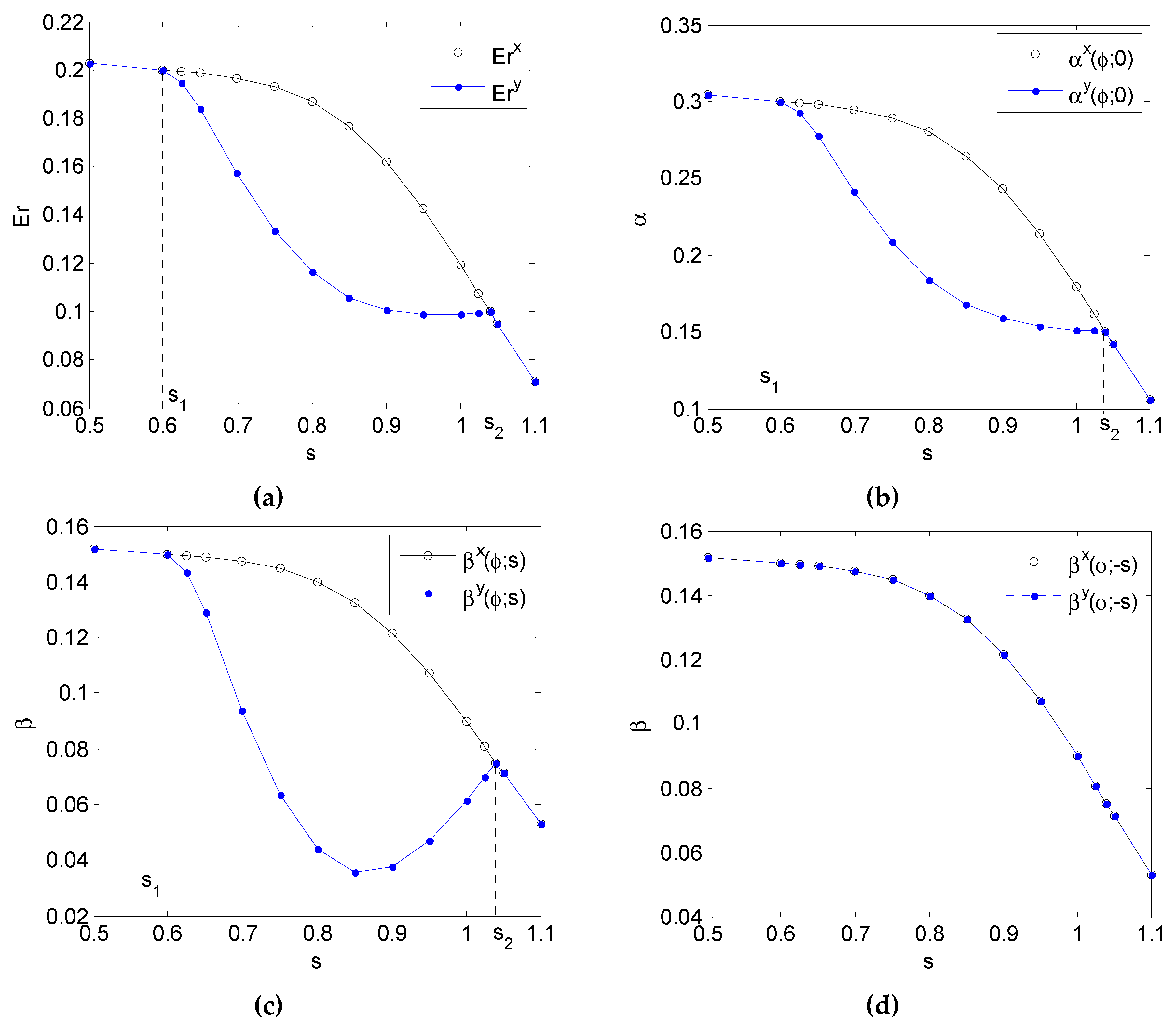
4.1. Rayleigh Distribution Background Noise

Suppose that $\mathrm{\Theta }=s$ is a constant, the problem shown in (39) represents a simple binary hypothesis testing problem. Here, we set $d_0=d_2=0$ and $d_1=1$, then the detector becomes

$$T(y)=y\stackrel{H_1}{\underset{H_0}{\underset{<}{>}}}\gamma$$

(41)

It is assumed that the background noise $v$ obeys the mixture of Rayleigh distributions with zero-means such that $p_v(v)={\displaystyle {\sum }_{i=1}^M{m}_i{\phi }_i(v-{\mu }_i)}$, where $m_i\ge 0$ for $i=1,\dots ,M$, ${\displaystyle {\sum }_{i=1}^M{m}_i}=1$, and

$${\phi }_i(x)=\{\begin{array}{ll}\frac{x}{{\sigma }_i^2}\exp (-\frac{x^2}{2{\sigma }_i^2}),& x\ge 0\\ 0,& x<0\end{array}$$

(42)

In the simulations, the variances of all the Rayleigh components are assumed to be the same, i.e., ${\sigma }_i=\sigma$ for $i=1,\dots ,M$. In addition, the parameters are specified as $M=4$, $u_1=0.2$, $u_2=0.4$, $u_3=-2\sigma \sqrt{\frac{\pi }{2}}-0.2$, $u_4=-2\sigma \sqrt{\frac{\pi }{2}}-0.4$ and $m_i=0.25$ for $i=1,\dots ,4$. From (33) and (34), the noise modified type I error probability $A_0(n)$ and type II error probability $B_1(n)$ obtained by adding a constant vector $n$ is calculated as:

$$A_0(n)={\displaystyle {\int }_{\gamma }^{+\infty }{f}_0(y)dy=}{\displaystyle \sum _{i=1}^4{m}_i}\mathrm{\Phi }(\gamma -{\mu }_i-n)$$

(43)

$$B_1(n)={\displaystyle {\int }_{-\infty }^{\gamma }{f}_1(y)dy=}1-{\displaystyle \sum _{i=1}^4{m}_i}\mathrm{\Phi }(\gamma -{\mu }_i-n-s)$$

(44)

where $\mathrm{\Phi }(x)={\displaystyle {\int }_x^{\infty }\frac{x}{{\sigma }^2}\exp (-\frac{x^2}{2{\sigma }^2})}dt$, when $x>0$; $\mathrm{\Phi }(x)=1$, when $x\le 0$. Accordingly, ${\alpha }^x=A_0(0)$ $={\displaystyle {\sum }_{i=1}^4{m}_i\mathrm{\Phi }(\gamma -{\mu }_i)}$ and ${\beta }^x=B_1(0)=1-{\displaystyle {\sum }_{i=1}^4{m}_i\mathrm{\Phi }(\gamma -{\mu }_i-s)}$. Let $c_1={\beta }^x/({\alpha }^x+{\beta }^x)$ and $c_2=$ ${\alpha }^x/({\alpha }^{\mathbf{x}}+{\beta }^x)$, the noise modified weighted sum of the two types of error probabilities obtained via adding a constant vector is $Er(n)=c_1{\displaystyle {\sum }_{i=1}^4{m}_i\mathrm{\Phi }(\gamma }-{\mu }_i-n)+c_2{\displaystyle {\sum }_{i=1}^4{m}_i\mathrm{\Phi }(\gamma -{\mu }_i}-n-s)$.

From Section 3.2, the pdf of the optimal additive noise that minimizes weighted sum of type I and II error probabilities is denoted by $p_{\mathbf{n}}^{opt}(\mathbf{n})=\eta \delta (\mathbf{n}-{\mathbf{n}}_1)+(1-\eta )\delta (\mathbf{n}-{\mathbf{n}}_2)$, under the two constraints that ${\alpha }^y\le {\alpha }^x$ and ${\beta }^y\le {\beta }^x$. Moreover, the optimal additive noise for the case without any constraints is a constant vector.

Figure 1 plots the minimum noise modified weighted sums of type I and II error probabilities obtained under no constraint and two constraints that ${\alpha }^y\le {\alpha }^x$ and ${\beta }^y\le {\beta }^x$, and the original weighted sum without adding any noise for different values of $\sigma$ when $s=3$ and $\gamma =s/2$. When $\sigma \le {\sigma }_1$, there is no noise that decreases the weighted sum. With the increase of $\sigma$, noise exhibits a positive effect on the detection performance. To be specific, when ${\sigma }_1<\sigma <{\sigma }_2$, the weighted sum can be decreased by adding a constant vector for the no constraint case. When $\sigma >{\sigma }_2$, the weighted sum can be decreased adding the noise under two constraints. The noise modified weighted sum obtained without any constraints is less than or equal to that obtained under the two constraints, and the difference between them first decreases to zero for ${\sigma }_3<\sigma <{\sigma }_4$ and then gradually increases when $\sigma >{\sigma }_4$. In addition, once $\sigma$ exceeds a certain value, no noise exists that can decrease the weighted sum for any cases.

Figure 1. The minimum noise modified weighted sums of the type I and II error probabilities obtained under no constraint and two constraints, and the original weighted sum for different $\sigma$ when s = 3 and γ = s/2.

Figure 2 shows the type I and II error probabilities corresponding to the weighted sum in Figure 1. From both Figure 1 and Figure 2, it is observed that one of the noise modified Type I and II error probabilities performs worse than the original one for the no constraint case. Therefore, though the noise modified weighted sum obtained with no constraint is less than that obtained under the two constraints, the corresponding noise is actually not suitable to add to the observation. Furthermore, when the minimum value of the noise modified weighted sum is obtained under the two constraints, the corresponding type II probability equals to the original one and the type I probability achieves the minimum for ${\sigma }_2<\sigma <{\sigma }_3$. Conversely, when $\sigma >{\sigma }_4$, the corresponding type I probability equals to the original one and the type II probability achieves the minimum. The results are consistent with part (3) and part (4) in Theorem 5. Especially, for ${\sigma }_3<\sigma <{\sigma }_4$, the minimum values of the noise modified weighted sum obtained under no constraint is equal to that obtained under two constraints, and the corresponding type I and II error probabilities are the same, which also agrees with part (2) in Theorem 5. In order to further illustrate the results in Figure 1 and Figure 2, Table 1 provides the optimal additive noises added for the two different cases.

Figure 2. The type I (a) and II (b) error probabilities corresponding to the weighted sum in Figure 1.

Table 1. The optimal additive noises that minimize the weighted sum under two constraints and no constraint for various $\sigma$ where s = 3 and γ = s/2.

$\mathit{\sigma }$	Two Constraints			No Constraints
	${\mathit{n}}_{\mathbf{1}}$	${\mathit{n}}_{\mathbf{2}}$	$\eta$	${\mathit{n}}_{\mathit{o}}$
0.950	-	-	-	−1.7089
1.250	−1.9082	1.7963	0.6950	−1.9218
2.125	−2.5136	3.1896	0.7862	−2.5136/3.1896
3.000	−3.3771	4.6942	0.3770	4.7449

Figure 3 depicts the minimum noise modified weighted sums of the type I and II error probabilities versus $s$ for the cases of no constraint and two constraints, and the original weighted sum, when $\sigma =1$ and $\gamma =s/2$. The corresponding type I and II error probabilities are depicted in Figure 4a,b, respectively. It is seen in Figure 3, the improvement of the weighted sum obtained by adding noise first increases and then decreases with the increase of $s$, and finally they all converge to the same value. The differences for the cases with and without constraints are very small in most cases. In the small interval of $s$, i.e., $s\in (s_1,s_2)$, the difference even decreases to zero. On the other hand, the noise modified type I error probability obtained under no constraint is significantly greater than the original one for $s<s_1$, while the corresponding type II error probability is less than that obtained under the two constraints. The situation, however, is reversed for $s_2<s<s_3$. When $s>s_3$, there is no noise that decreases the weighted sum under the two constraints, while the weighted sum is still decreased by adding a constant vector for no constraint case. When $s>s_4$, the weighted sum cannot be decreased by adding any noise for all the cases. Furthermore, Table 2 shows the optimal additive noises that minimize the weighted sum under the cases of no and two constraints.

Figure 3. The minimum noise modified weighted sums of the type I and II error probabilities obtained under no constraint and two constraints, and the original weighted sum for different $s$ when σ = 1 and γ = s/2.

Figure 4. The type I and II error probabilities corresponding to the weighted sum in Figure 3 are shown in (a) and (b), respectively.

Table 2. The optimal additive noises that minimize the weighted sum under two constraints and no constraint for various $s$ where σ = 1 and γ = s/2.

$\mathit{s}$	Two Constraints			No Constraints
	${\mathit{n}}_{\mathbf{1}}$	${\mathit{n}}_{\mathbf{2}}$	$\mathit{\eta }$	${\mathit{n}}_{\mathit{o}}$
1.25	−1.3682	1.7327	0.2918	1.7474
1.75	−1.4408	1.6563	0.7265	−1.4408/1.6563
2.5	−1.6052	1.4690	0.6983	−1.6201
3.25	-	-	-	−0.5866

Figure 5 shows the minimum noise modified weighted sums of type I and II error probabilities versus $\gamma$ for the cases of no constraint and two constraints, and the original weighted sum, when $\sigma =1$ and $s=3$. The corresponding type I and II error probabilities are depicted in Figure 6a,b, respectively. As illustrated in Figure 5, when $\gamma$ is close to zero, the original weighted sum $E{r}^x$ approaches to zero. In such case, no additive noise exists to decrease the weighted sum. For the case of two constraints, the improvement of the weighted sum first increases for ${\gamma }_1<\gamma <{\gamma }_2$ and then decreases for ${\gamma }_2<\gamma <{\gamma }_3$, and no improvement can be obtained when $\gamma >{\gamma }_2$. On the other hand, the minimum noise modified weighted sum obtained under no constraint is smaller than that obtained under the two constraints for ${\gamma }_1<\gamma <{\gamma }_3$, and the difference between them first increases and then decreases for both ${\gamma }_1<\gamma <{\gamma }_2$ and ${\gamma }_2<\gamma <{\gamma }_3$. When $\gamma >{\gamma }_3$, there still exists a constant vector that decreases the weighted sum, but it may be not a suitable noise in the practical application according to the type II probability depicted in Figure 6b. Furthermore, in order to study the results illustrated in Figure 5 and Figure 6, Table 3 shows the optimal additive noises that minimize the weighted sum for the cases of no and two constraints.

Figure 5. The minimum noise modified weighted sums of the type I and II error probabilities obtained under no constraint and two constraints, and the original weighted sum for different $\gamma$ when σ = 1 and s = 3.

Figure 6. The type I and II error probabilities corresponding to the weighted sum in Figure 5 are shown in (a) and (b), respectively.

Table 3. The optimal additive noises that minimize the weighted sum under two constraints and no constraint for various $\gamma$ where σ = 1 and s = 3.

$\mathit{\gamma }$	Two Constraints			No Constraints
	${\mathit{n}}_{\mathbf{1}}$	${\mathit{n}}_{\mathbf{2}}$	$\mathit{\eta }$	${\mathit{n}}_{\mathit{o}}$
0.050	-	-	-	-
1.100	−2.1213	0.9341	0.2878	0.9691
1.425	−1.7947	1.2585	0.5355	−1.7957
2.250	−0.9693	2.0836	0.8867	−1.1763
3.375	-	-	-	−0.5775

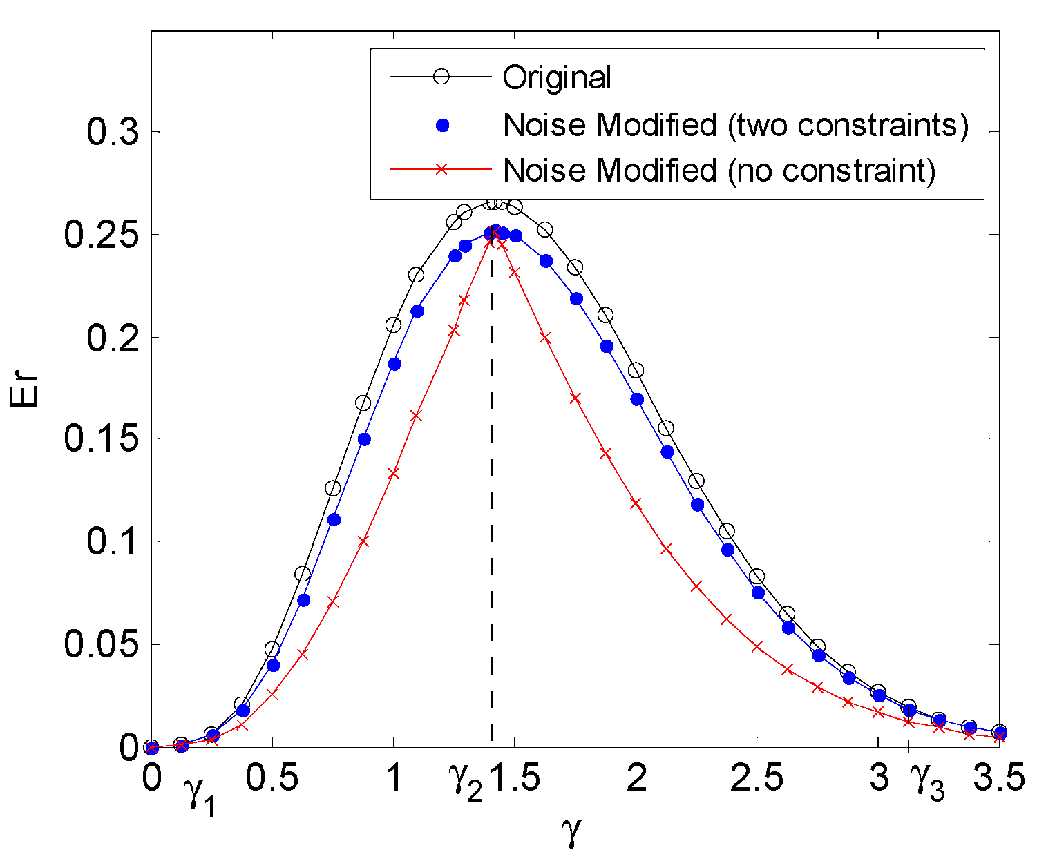
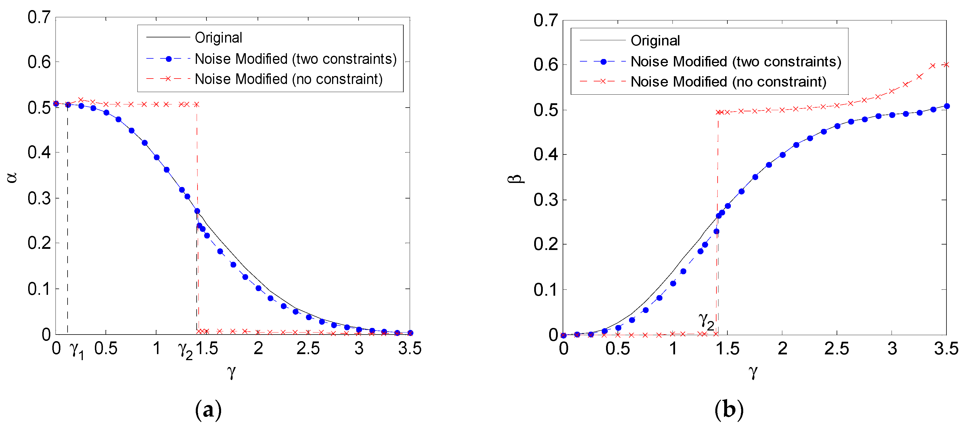
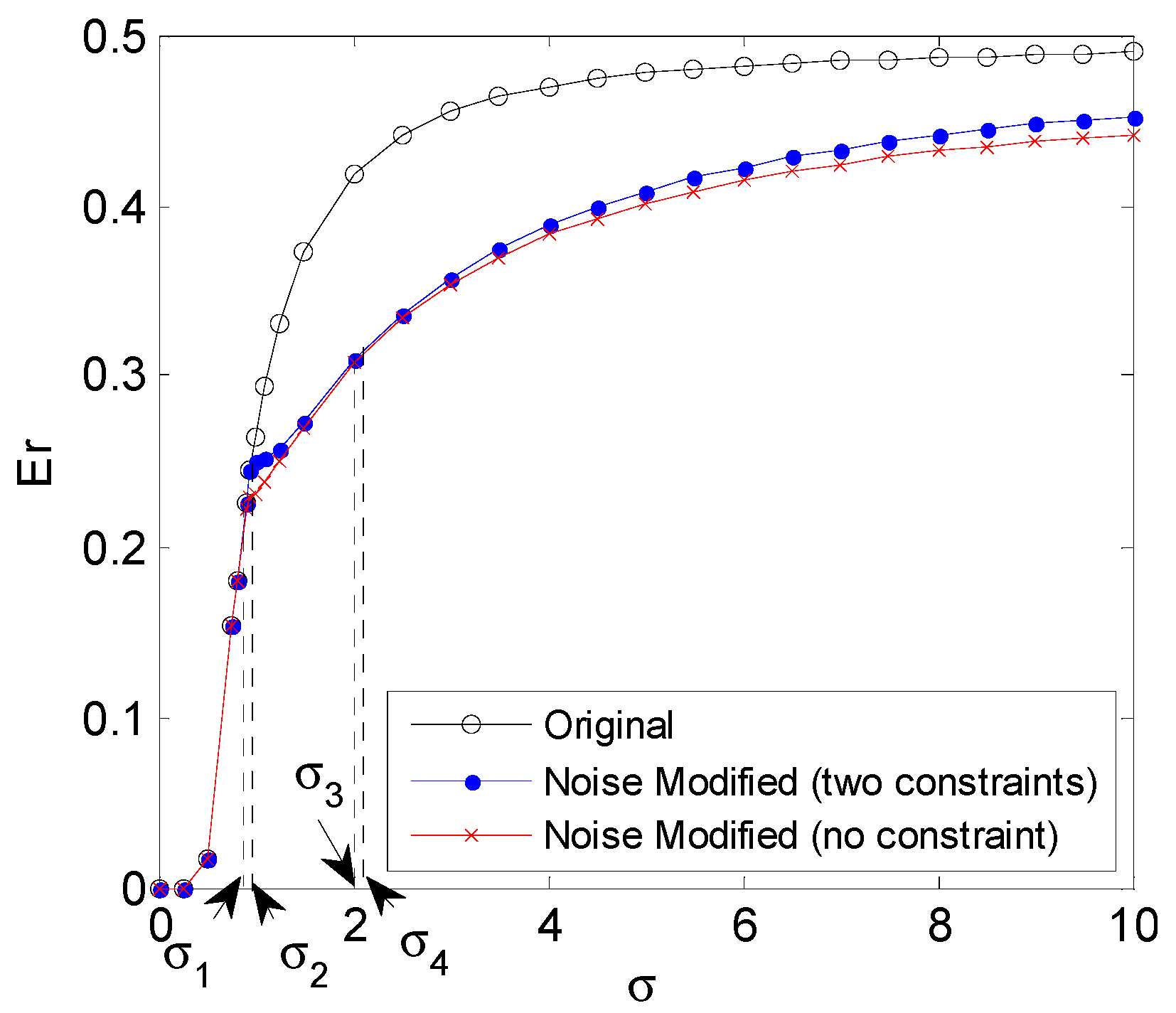
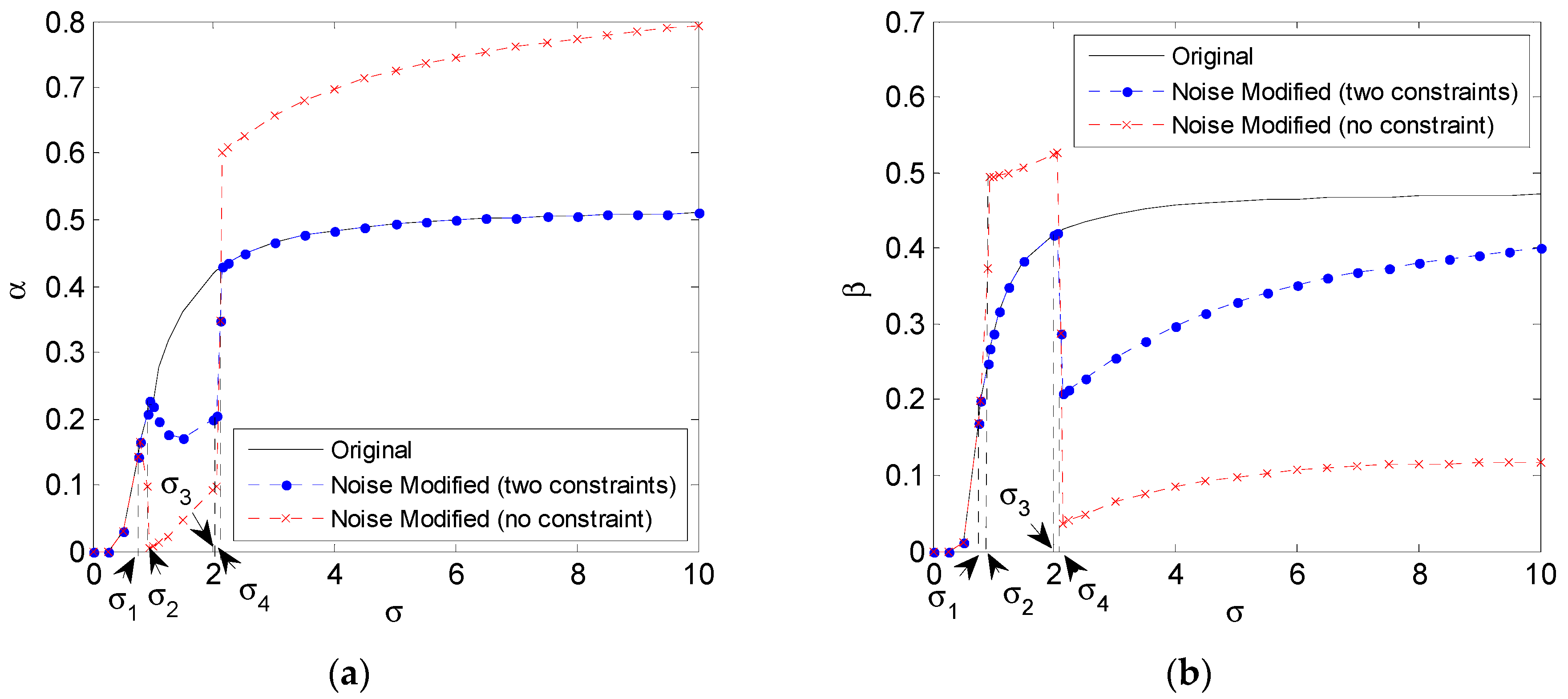
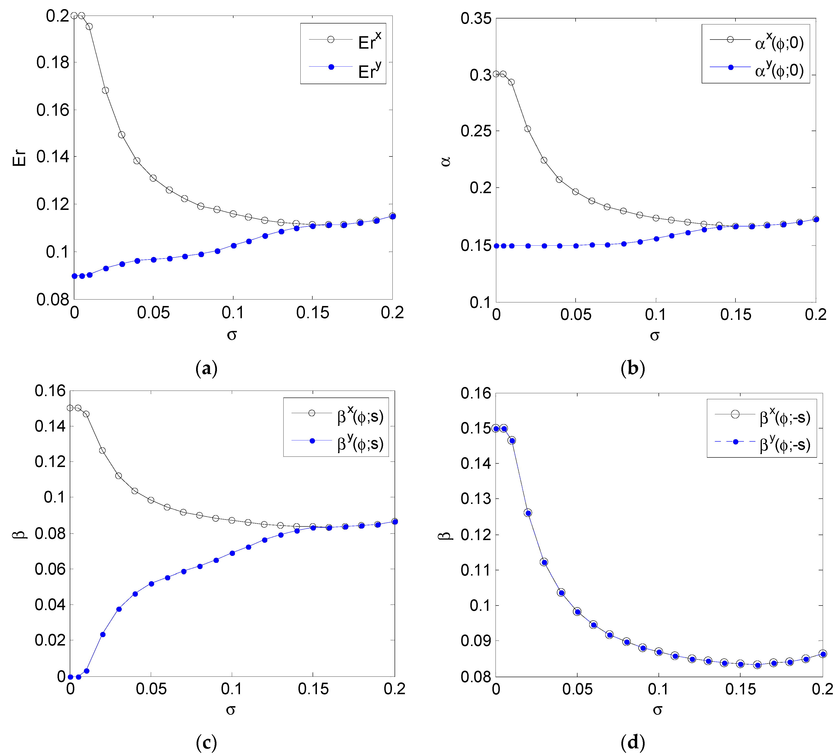
4.2. Gaussian Mixture Background Noise

Suppose that $\mathrm{\Theta }$ is a random variable with following pdf:

$${\varpi }_1(\theta )=\rho \delta (\theta -s)+(1-\rho )\delta (\theta +s)$$

(45)

Therefore, we have ${\mathrm{\Omega }}_0=\{0\}$ and ${\mathrm{\Omega }}_1=\{s,-s\}$. In the simulations, we set $d_0=1$, $d_1=0$, $d_2=-s^2/4$ and $\gamma =0$, the detector is expressed as:

$$T(y)=y^2-\frac{s^2}{4}\stackrel{H_1}{\underset{H_0}{\underset{<}{>}}}0$$

(46)

Moreover, we assume that $v$ is a zero-mean symmetric Gaussian mixture noise with pdf of $p_v(v)={\displaystyle {\sum }_{i=1}^M{m}_i{\psi }_i(v-{\mu }_i)}$, where $m_i\ge 0$, ${\displaystyle {\sum }_{i=1}^M{m}_i}=1$ and:

$${\psi }_i(v)=\frac{1}{\sqrt{2\pi {\sigma }_i^2}}\exp (-\frac{v^2}{2{\sigma }_i^2})$$

(47)

Let $M=4$ and the mean values of the symmetric Gaussian components are set as [0.05 0.52 −0.52 −0.05] with corresponding weights [0.35 0.15 0.15 0.35]. In addition, the variances of Gaussian components are the same, i.e., ${\sigma }_i=\sigma$ for $i=0,\dots ,4$. According to (12) and (14), the noise modified type I error probability obtained by adding a constant vector $n$ to $x$ is calculated by:

$$A_0(n)={\displaystyle \sum _{i=1}^4{m}_i}(\Psi (\frac{s/2+{\mu }_i+n}{\sigma })+\Psi (\frac{s/2-{\mu }_i-n}{\sigma }))$$

(48)

and the corresponding type II error probabilities for $\mathrm{\Theta }=s$ and $-s$ are respectively calculated as:

$$B_s(n)=1-{\displaystyle \sum _{i=1}^4{m}_i}(\Psi (\frac{3s/2+{\mu }_i+n}{\sigma })+\Psi (\frac{-s/2-{\mu }_i-n}{\sigma }))$$

(49)

$$B_{-s}(n)=1-{\displaystyle \sum _{i=1}^4{m}_i}(\Psi (\frac{-s/2+{\mu }_i+n}{\sigma })+\Psi (\frac{3s/2-{\mu }_i-n}{\sigma }))$$

(50)

where $\Psi (x)={\displaystyle {\int }_x^{\infty }\frac{1}{\sqrt{2\pi }}\exp (-\frac{t^2}{2{\sigma }^2})}dt$. Accordingly:

$$B_1(n)=\rho B_s(n)+(1-\rho )B_{-s}(n)$$

(51)

Therefore, the original type I and type II error probabilities for $\mathrm{\Theta }=s$ and $-s$ are ${\alpha }^x(\varphi ;0)=A_0(0)$, ${\beta }^x(\varphi ;s)=B_s(0)$ and ${\beta }^x(\varphi ;-s)=B_{-s}(0)$, respectively.

Due to the symmetry property of $v$, one obtains $B_s(0)=B_{-s}(0)$. In this case, the original average type II error probability is ${\beta }^x=B_1(0)=\rho {\beta }^x(\varphi ;s)+(1-\rho ){\beta }^x(\varphi ;-s)=B_s(0)=B_{-s}(0)$. The noise modified weighted sum of type I and average type II error probabilities corresponding to the constant vector is expressed by $Er(n)=c_1{A}_0(n)+c_2{B}_1(n)$. The values of $c_1$ and $c_2$ are still specified as ${\beta }^x/({\alpha }^x+{\beta }^x)$ and ${\alpha }^x/({\alpha }^x+{\beta }^x)$, respectively. From Theorem 4 in Section 2.3, the optimal additive noise that minimizes the weighted sum is a randomization with a pdf of $p_n^{opt}(n)={\eta }_1\delta (n-n_1)+{\eta }_2\delta (n-n_2)+{\eta }_3\delta (n-n_3)$, where ${\eta }_i\ge 0$ for $i=1,\dots ,3$, and ${\displaystyle {\sum }_{i=1}^3{\eta }_i}=1$.

Figure 7 shows the detection performance of the original detector and the noise enhanced detector that minimizes the weighted sum of type I and average type II error probabilities under the constraints that ${\alpha }^y(\varphi ;0)\le {\alpha }_o$ and $\underset{\theta \in {\mathrm{\Omega }}_1}{\max }{\beta }^y(\varphi ;\theta )\le {\beta }_o$, for different values of $\sigma$ where $s=1$ and $\rho =0.6$. The minimum achievable noise modified weighted sum is plotted in Figure 7a, and the corresponding type I error probability and type II error probabilities for $\mathrm{\Theta }=s$ and $-s$ are depicted in Figure 7b–d, respectively.

Figure 7. The weighted sums, type I error probabilities, and type II error probabilities for $\mathrm{\Theta }=s$ and −s of the original detector and the noise enhanced detector for different σ where s = 1 and ρ = 0.6 shown in (a), (b), (c) and (d), respectively

From Figure 7, the original weighted sums, type I error probabilities, and type II error probabilities for $\mathrm{\Theta }=s$ and $-s$ increase as $\sigma$ decreases towards zero. In Figure 7a, when $\sigma$ is close to zero, the weighted sum can be decreased significantly. With the increase of $\sigma$, the improvement obtained by adding noise is reduced gradually to zero. In other words, the phenomenon of noise-enhanced detection performance cannot occur when $\sigma$ exceeds a certain value. In Figure 7b, the noise modified type I error probability stays at 0.1500 for $\sigma <0.07$ and then increases gradually to equal to the original type I error probability. Moreover, the noise modified type II error probabilities for $\mathrm{\Theta }=s$ corresponding to the minimum weighted sum increases from zero to that of original detector, shown in Figure 7c, while the type II error probabilities for $\mathrm{\Theta }=-s$ of the noise enhanced detector is equal to that of the original detector all the time. In fact, the type II error probability for $\mathrm{\Theta }=s$ also reaches the minimums under the constraints that ${\alpha }^y(\varphi ;0)\le {\alpha }_o$ and $\underset{\theta \in {\mathrm{\Omega }}_1}{\max }{\beta }^y(\varphi ;\theta )\le {\beta }_o$ in this example. In addition, Table 4 offers the optimal additive noises that minimize the weighted sum for different values of $\sigma$ to explain the results in Figure 7. It should be noted that the optimal noise is not unique.y.

Table 4. The optimal additive noises that minimize the weighted sum under two constraints for various $\sigma$ where s = 1 and ρ = 0.6.

$\mathit{\sigma }$	${\mathit{n}}_{\mathbf{1}}$	${\mathit{n}}_{\mathbf{2}}$	${\mathit{n}}_{\mathbf{3}}$	${\mathit{\eta }}_{\mathbf{1}}$	${\mathit{\eta }}_{\mathbf{2}}$	${\mathit{\eta }}_{\mathbf{3}}$
0.0001	0.2286	-	-	1.0000	-	-
0.02	0.2286	−0.2255	-	0.8413	0.1587	-
0.05	0.2287	−0.2208	0.2421	0.5310	0.3446	0.1244
0.08	0.2180	−0.2185	−0.2168	0.5943	0.2449	0.1608

Figure 8a demonstrates the weighted sums of type I and average type II error probabilities of the original detector and the noise enhanced detector versus $s$, where $\sigma =0.08$ and $\rho =0.6$. The corresponding type I error probability and type II error probabilities for $\mathrm{\Theta }=s$ and $-s$ are depicted in Figure 8b–d, respectively. From Figure 8a, the weighted sum cannot be decreased under the constraints on different error probabilities for $s<s_1$ and $s<s_2$. Conversely, there exists additive noise under the constraints that reduces the weighted sum for $s_1<s<s_2$, and the corresponding improvement first increases and then decreases with the increase of $s$. Comparing Figure 8b with Figure 8a, it is noted that the change of the noise modified type I error probability is similar to that of the noise modified weighted sum. In Figure 8c, the noise modified type II error probability for $\mathrm{\Theta }=s$ first decreases to the minimum and then increases as $s$ increases, while the type II error probability for $\mathrm{\Theta }=-s$ of the noise modified detector is always equal to that of the original detector, shown in Figure 8d. In addition, in order to further illustrate the results in Figure 8, Table 5 shows the optimal noises that minimize the weighted sum under the case of two constraints.

Figure 8. The weighted sums, type I error probabilities, and type II error probabilities for $\mathrm{\Theta }=s$ and −s of the original detector and the noise enhanced detector for different s where σ = 0.08 and ρ = 0.6 shown in (a), (b), (c) and (d), respectively.

Table 5. The optimal additive noises that minimize the weighted sum under two constraints for various $s$ where σ = 0.08 and ρ = 0.6.

$\mathit{s}$	${\mathit{n}}_1$	${\mathit{n}}_2$	${\mathit{n}}_3$	${\mathit{\eta }}_1$	${\mathit{\eta }}_2$	${\mathit{\eta }}_3$
0.65	0.1613	−0.1613	-	0.6267	0.3733	-
0.75	0.2026	−0.2026	-	0.7949	0.2051	-
0.85	0.2148	−0.2149	-0.2150	0.8262	0.1300	0.0438
0.95	0.2195	−0.2196	-0.2190	0.7006	0.1916	0.1078

5. Conclusions

In this paper, a noise-enhanced detection problem has been investigated for a general composite hypothesis testing. Under the constraints of type I and II error probabilities, the minimization of the weighted sum of average type I and II error probabilities has been explored by adding an additive independent noise. The sufficient conditions for improvability of the weighted sum are provided, and a simple algorithm to search the optimal noise is developed. Then some additional theoretical results are made based on the specificity of the binary simple hypothesis testing problem. The studies on different noise distributions confirm the theoretical analysis that the optimal additive noise indeed minimizes the weighted sum under certain conditions. To be noted that, theoretical results can also be extended to a broad class of noise enhanced optimization problems under two inequality constraints such as the minimization of Bayes risk under the different constraints of condition risks for a binary hypothesis testing problem.

References

- DeGroot, M.H.; Sxhervish, M.J. Probability and Statistics, 4nd ed.; Addison-Wesley: Boston, MA, USA, 2011. [Google Scholar]
- Pericchi, L.; Pereira, C. Adaptative significance levels using optimal decision rules: Balancing by weighting the error probabilities. Braz. J. Probab. Stat. 2016, 30, 70–90. [Google Scholar] [CrossRef]
- Benzi, R.; Sutera, A.; Vulpiani, A. The mechanism of stochastic resonance. J. Phys. A Math. 1981, 14, 453–457. [Google Scholar] [CrossRef]
- Patel, A.; Kosko, B. Noise benefits in quantizer-array correlation detection and watermark decoding. IEEE Trans. Signal Process. 2011, 59, 488–505. [Google Scholar] [CrossRef]
- Han, D.; Li, P.; An, S.; Shi, P. Multi-frequency weak signal detection based on wavelet transform and parameter compensation band-pass multi-stable stochastic resonance. Mech. Syst. Signal Process. 2016, 70–71, 995–1010. [Google Scholar] [CrossRef]
- Addesso, P.; Pierro, V.; Filatrella, G. Interplay between detection strategies and stochastic resonance properties. Commun. Nonlinear Sci. Numer. Simul. 2016, 30, 15–31. [Google Scholar] [CrossRef]
- Gingl, Z.; Makra, P.; Vajtai, R. High signal-to-noise ratio gain by stochastic resonance in a double well. Fluct. Noise Lett. 2001, 1, L181–L188. [Google Scholar] [CrossRef]
- Makra, P.; Gingl, Z. Signal-to-noise ratio gain in non-dynamical and dynamical bistable stochastic resonators. Fluct. Noise Lett. 2002, 2, L147–L155. [Google Scholar] [CrossRef]
- Makra, P.; Gingl, Z.; Fulei, T. Signal-to-noise ratio gain in stochastic resonators driven by coloured noises. Phys. Lett. A 2003, 317, 228–232. [Google Scholar] [CrossRef]
- Duan, F.; Chapeau-Blondeau, F.; Abbott, D. Noise-enhanced SNR gain in parallel array of bistable oscillators. Electron. Lett. 2006, 42, 1008–1009. [Google Scholar] [CrossRef]
- Mitaim, S.; Kosko, B. Adaptive stochastic resonance in noisy neurons based on mutual information. IEEE Trans. Neural Netw. 2004, 15, 1526–1540. [Google Scholar] [CrossRef] [PubMed]
- Patel, A.; Kosko, B. Mutual-Information Noise Benefits in Brownian Models of Continuous and Spiking Neurons. In Proceedings of the 2006 International Joint Conference on Neural Network, Vancouver, BC, Canada, 16–21 July 2006; pp. 1368–1375. [Google Scholar]
- Chen, H.; Varshney, P.K.; Kay, S.M.; Michels, J.H. Theory of the stochastic resonance effect in signal detection: Part I – fixed detectors. IEEE Trans. Signal Process. 2007, 55, 3172–3184. [Google Scholar] [CrossRef]
- Patel, A.; Kosko, B. Optimal noise benefits in Neyman–Pearson and inequality constrained signal detection. IEEE Trans. Signal Process. 2009, 57, 1655–1669. [Google Scholar]
- Bayram, S.; Gezici, S. Stochastic resonance in binary composite hypothesis-testing problems in the Neyman–Pearson framework. Digit. Signal Process. 2012, 22, 391–406. [Google Scholar] [CrossRef]
- Bayrama, S.; Gultekinb, S.; Gezici, S. Noise enhanced hypothesis-testing according to restricted Neyman–Pearson criterion. Digit. Signal Process. 2014, 25, 17–27. [Google Scholar] [CrossRef]
- Bayram, S.; Gezici, S.; Poor, H.V. Noise enhanced hypothesis-testing in the restricted Bayesian framework. IEEE Trans. Signal Process. 2010, 58, 3972–3989. [Google Scholar] [CrossRef]
- Bayram, S.; Gezici, S. Noise enhanced M-ary composite hypothesis-testing in the presence of partial prior information. IEEE Trans. Signal Process. 2011, 59, 1292–1297. [Google Scholar] [CrossRef]
- Chen, H.; Varshney, L.R.; Varshney, P.K. Noise-enhanced information systems. Proc. IEEE 2014, 102, 1607–1621. [Google Scholar] [CrossRef]
- Weber, J.F.; Waldman, S.D. Stochastic Resonance is a Method to Improve the Biosynthetic Response of Chondrocytes to Mechanical Stimulation. J. Orthop. Res. 2015, 34, 231–239. [Google Scholar] [CrossRef] [PubMed]
- Duan, F.; Chapeau-Blondeau, F.; Abbott, D. Non-Gaussian noise benefits for coherent detection of narrow band weak signal. Phys. Lett. A 2014, 378, 1820–1824. [Google Scholar] [CrossRef]
- Lu, Z.; Chen, L.; Brennan, M.J.; Yang, T.; Ding, H.; Liu, Z. Stochastic resonance in a nonlinear mechanical vibration isolation system. J. Sound Vib. 2016, 370, 221–229. [Google Scholar] [CrossRef]
- Rossi, P.S.; Ciuonzo, D.; Ekman, T.; Dong, H. Energy Detection for MIMO Decision Fusion in Underwater Sensor Networks. IEEE Sen. J. 2015, 15, 1630–1640. [Google Scholar] [CrossRef]
- Rossi, P.S.; Ciuonzo, D.; Kansanen, K.; Ekman, T. Performance Analysis of Energy Detection for MIMO Decision Fusion in Wireless Sensor Networks Over Arbitrary Fading Channels. IEEE Trans. Wirel. Commun. 2016, 15, 7794–7806. [Google Scholar] [CrossRef]
- Ciuonzo, D.; de Maio, A.; Rossi, P.S. A Systematic Framework for Composite Hypothesis Testing of Independent Bernoulli Trials. IEEE Signal Proc. Lett. 2015, 22, 1249–1253. [Google Scholar] [CrossRef]
- Parsopoulos, K.E.; Vrahatis, M.N. Particle Swarm Optimization Method for Constrained Optimization Problems; IOS Press: Amsterdam, The Netherlands, 2002; pp. 214–220. [Google Scholar]
- Hu, X.; Eberhart, R. Solving constrained nonlinear optimization problems with particle swarm optimization. In Proceedings of the sixth world multiconference on systemics, cybernetics and informatics, Orlando, FL, USA, 14–18 July 2002. [Google Scholar]
- Price, K.V.; Storn, R.M.; Lampinen, J.A. Differential Evolution: A Practical Approach to Global Optimization; Springer: New York, NY, USA, 2005. [Google Scholar]
© 2017 by the authors. Licensee MDPI, Basel, Switzerland. This article is an open access article distributed under the terms and conditions of the Creative Commons Attribution (CC BY) license (http://creativecommons.org/licenses/by/4.0/).