Using k-Mix-Neighborhood Subdigraphs to Compute Canonical Labelings of Digraphs

Abstract

This paper presents a novel theory and method to calculate the canonical labelings of digraphs whose definition is entirely different from the traditional definition of Nauty. It indicates the mutual relationships that exist between the canonical labeling of a digraph and the canonical labeling of its complement graph. It systematically examines the link between computing the canonical labeling of a digraph and the k-neighborhood and k-mix-neighborhood subdigraphs. To facilitate the presentation, it introduces several concepts including mix diffusion outdegree sequence and entire mix diffusion outdegree sequences. For each node in a digraph G, it assigns an attribute m_NearestNode to enhance the accuracy of calculating canonical labeling. The four theorems proved here demonstrate how to determine the first nodes added into $MaxQ(G)$. Further, the other two theorems stated below deal with identifying the second nodes added into $MaxQ(G)$. When computing $C_{max}(G)$, if $MaxQ(G)$ already contains the first i vertices $u_1,u_2,\cdots ,u_i$, Diffusion Theorem provides a guideline on how to choose the subsequent node of $MaxQ(G)$. Besides, the Mix Diffusion Theorem shows that the selection of the $(i+1)$th vertex of $MaxQ(G)$ for computing $C_{max}(G)$ is from the open mix-neighborhood subdigraph $N^{++}(Q)$ of the nodes set $Q=\{u_1,u_2,\cdots ,u_i\}$. It also offers two theorems to calculate the $C_{max}(G)$ of the disconnected digraphs. The four algorithms implemented in it illustrate how to calculate $MaxQ(G)$ of a digraph. Through software testing, the correctness of our algorithms is preliminarily verified. Our method can be utilized to mine the frequent subdigraph. We also guess that if there exists a vertex $v\in S^{+}(G)$ satisfying conditions $C_{max}(G-v)⩽C_{max}(G-w)$ for each $w\in S^{+}(G)\wedge w\ne v$, then $u_1=v$ for $MaxQ(G)$.

1. Introduction

A canonical labeling [1,2,3] of a graph, also called a canonical form [4], a canonical code [5], or an optimum code [6], is a unique string corresponding to the graph and is lexicographically smallest or largest according to the different definitions used in the studies. Two digraphs are isomorphic if and only if they have the same canonical labelings. Until now, the computation of the canonical labeling as the digraph isomorphism problem remains an unsolved problem in computational complexity theory in the sense that no polynomial-time algorithm exists for calculating the canonical labeling of a digraph. Therefore, the computation of the canonical labeling is NP-hard [4,7].

Numerous methods have emerged to calculate the canonical labelings of undirected graphs. However, different methods use distinct definitions of the canonical labeling. Given a graph with n vertices, Huan et al. concatenates the lower triangular entries (including the diagonal entries) of its adjacency matrix to produce its canonical labeling [8]. Kuramochi and Karypis construct the canonical labeling by concatenating the columns of the upper-triangular portion of its adjacency matrix [9,10]. To create the canonical labeling, He et al. concatenate the rows of its adjacency matrix to form a $n^2$ binary number [11,12].

Babai and Luks pioneered the establishment of a general group-theoretic approach to compute canonical labeling [4]. However, combinatorial methods have worked well in various special cases. For random graphs, Babai et al. produce a canonical labeling with high probability [4,13]. Arvind et al. propose two corresponding logspace algorithms for partial 2- and 3-Trees [7,14].

Jianqiang Hao establishes a new theoretical framework to compute the canonical labeling $C_{max}(G)$ of undirected graphs by defining a set of concepts useful for classifying graphs [15].

Currently, Nauty [1,16,17,18] is the most popular and practical tools for considering the automorphism group and the canonical label of a graph or digraph. On isomorphism testing, Nauty is more efficient than Ullmann [19]. It has almost become the industry standard used to calculate the canonical label, as well as the automorphism group. For computing the canonical labeling and automorphism group, Nauty and [20] use the depth-first search to traverse the potential intermediate nodes in the search tree. The nodes of the search tree generated by Nauty are equitable ordered partitions of nodes in G. Nauty iteratively refines partitioning nodes until places the nodes that have the same properties into an automorphism orbit. As the partition refinement becomes finer and smaller, it automatically creates the canonical label. Nauty also requires exponential time to compute the canonical labeling for a given Miyazaki graph [21]. Tener and Deo [22] made improvements for dealing with the problem.

Besides Nauty, Bliss [3,23], Traces [2], and Conauto [24] are also state-of-the-art tools for graphs isomorphism testing. Based on backtracking, individualization of vertices, and partition refinement, Bliss [3,23] is an efficient canonical labeling tool for handling large and sparse graphs. Katebi et al. [25] can find the symmetry while calculating the canonical labeling. To fix the glitch of Nauty, Traces [2] uses the strategy of breadth-first search to find the automorphism group and the canonical labeling. Conauto also uses the basic individualization/refinement technique and is very fast for random graphs and several families of hard graphs.

For the improvement of performance, existing algorithms commonly utilize backtracking and orbit partitioning technique to avoid repeatedly visiting the same vertices, as well as manage to reduce the accessed nodes in the search tree. McKay and Piperno provides a comprehensive discussion of the issue [18].

Nauty dominated the field for several decades. As a result, an in-depth study for the canonical labeling has been confined to the theoretical framework of Nauty. This means that people just follow the research trajectory of nauty to extend and establish further study. When the graph under consideration contains a large number of automorphisms, it is difficult to verify the correctness of the canonical labeling obtained by performing Nauty according to the standard of Nauty.

Although many algorithms have emerged to calculate the canonical labelings of undirected graphs, to our best knowledge no algorithm other than Nauty exists for computing the canonical labelings of digraphs.

Throughout the paper, the canonical labeling $C_{max}(G)$ of a digraph is the lexicographically largest code obtained by concatenating the rows of the associated adjacency matrix (see Definition 7). Our definition of canonical labeling is entirely different from that of Nauty.

Although a few algorithms also give the same definition of the canonical labeling as described in Definition 7, their primary purpose is not to study how to construct a canonical labeling of a digraph, but for other intentions such as to mine the frequent subdigraphs. As a result, they can only work for some restricted undirected graph classes. Jianqiang Hao utilizes the $Cen(G)$ to calculate the first node $u_1$ added into $MaxQ(G)$ of simple undirected graphs [15]. Based on current knowledge and Definition 7, a general algorithm for computing the canonical labelings of digraphs is not available.

This paper focuses on the development of general theory and methods to calculate the canonical labeling $C_{max}(G)$ of digraphs. In the rest of this paper, Section 2 establishes some basic terminology and preliminary information. Section 3 describes the results accompanied by some discussion. Section 4 presents our algorithms for computing the canonical labeling of digraphs. Section 5 displays the implementation of our algorithms and evaluates our approach through many examples. Finally, Section 6 comments on our results and future work.

2. Preliminaries

In this section, we provide a brief review of the fundamental information used throughout the paper. A more comprehensive presentation can be found in most standard textbooks [26,27]. A directed graph (or digraph) $G=<V(G)$, $E(G)>$ consists of a nonempty set $V(G)$ of vertices (or nodes) and a set $E(G)$ of directed edges (or arcs). A directed edge associated with the ordered pair $(u,v)$ is said to start at u and end at v. We also say that the vertex u is its tail and the vertex v is its head. Throughout the paper, we denote $(u,v)$ by $u\to v$. For the edge $u\to v\in E(G)$, the vertex v is said to be adjacent from the vertex u, the vertex u is said to be adjacent to the vertex v, and the edge $u\to v$ is said to be incident from the vertex u and incident to the vertex v. The directed distance $\overrightarrow{d(u,v)}$ from vertex u to vertex v in G is the length of the shortest directed path from u to v [28], if any; otherwise $\overrightarrow{d(u,v)}=\infty$.

This paper deals with only finite simple digraphs, which have no loops and no multiple edges. For each $u\in V(G)$, let $d_G^{+-}(u)=|\{v|v\to u\wedge u\to v\in E(G)\}|$, $d_G^{+}(u)=|\{v|u\to v\in E(G)\}|$, $d_G^{-}(u)=|\{v|v\to u\in E(G)\}|$, and $d_G(u)=d_G^{+}(u)+d_G^{-}(u)$ denote the outindegree, outdegree, indegree, and degree of u respectively, and omit the subscript G when no ambiguity can arise. Denote by $\Delta (G)$, ${\Delta }^{+-}(G)$, ${\Delta }^{+}(G)$, and ${\Delta }^{-}(G)$ the maximum degree, the maximum outindegree, the maximum outdegree, and the maximum indegree of all vertices of a graph G, respectively.

Denote by $d(G)=(d_G(u_1)$, $d_G(u_2)$, ⋯, $d_G(u_n))$ the degree sequence of G, by $d_G(V_1)=(d_G(v_1)$, $d_G(v_2)$, ⋯, $d_G(v_m))$ the degree sequence of a subset $V_1\subseteq V(G)$ with $v_i\in V_1$, $i=1,2,\cdots ,m$, and by $d_G(H)=(d_H(w_1)$, $d_H(w_2)$, ⋯, $d_H(w_s))$ the degree sequence of a subdigraph $H\subseteq G$ with $w_j\in V(H)$, $j=1,2,\cdots ,s$, and omit the subscript G when no ambiguity can arise.

In addition, denote by $d^{+}(G)=(d_G^{+}(u_1)$, $d_G^{+}(u_2)$, ⋯, $d_G^{+}(u_n))$ the outdegree sequence of G, by $d_G^{+}(V_1)=(d_G^{+}(v_1)$, $d_G^{+}(v_2)$, ⋯, $d_G^{+}(v_m))$ the outdegree sequence of a subset $V_1\subseteq V(G)$ with $v_i\in V_1$, $i=1,2,\cdots ,m$, and by $d_G^{+}(H)=(d_H^{+}(w_1)$, $d_H^{+}(w_2)$, ⋯, $d_H^{+}(w_s))$ the outdegree sequence of a subdigraph $H\subseteq G$ with $w_j\in V(H)$, $j=1,2,\cdots ,s$, and omit the subscript G when no ambiguity can arise.

Similarly, denote by $d^{-}(G)=(d_G^{-}(u_1)$, $d_G^{-}(u_2)$, ⋯, $d_G^{-}(u_n))$ the indegree sequence of G, by $d_G^{-}(V_1)=(d_G^{-}(v_1)$, $d_G^{-}(v_2)$, ⋯, $d_G^{-}(v_m))$ the indegree sequence of a subset $V_1\subseteq V(G)$ with $v_i\in V_1$, $i=1,2,\cdots ,m$, and by $d_G^{-}(H)=(d_H^{-}(w_1)$, $d_H^{-}(w_2)$, ⋯, $d_H^{-}(w_s))$ the indegree sequence of a subdigraph $H\subseteq G$ with $w_j\in V(H)$, $j=1,2,\cdots ,s$, and omit the subscript G when no ambiguity can arise.

Throughout this paper, unless otherwise specified, any given degree sequence is non-increasing. Throughout this paper, let $S(G)=\{u|u\in V(G)\wedge d(u)=\Delta (G)\}$, $S^{+}(G)=\{u\in V(G)|d^{+}(u)={\Delta }^{+}(G)\}$, $S^{-}(G)=\{u\in V(G)|d^{-}(u)={\Delta }^{-}(G)\}$, and $S_{-}^{+}(G)=\{u\in S^{+}(G)|d^{-}(u)={\Delta }^{-}(S^{+}(G))\}$ where ${\Delta }^{-}(S^{+}(G))=\max \{d^{-}(u)|u\in S^{+}(G)\}$.

Definition 1.

Let $G=<V(G)$, $E(G)>$ be a simple digraph with n nodes. The vertex-induced subdigraph on $V_1\subseteq V(G)$ of G is the subdigraph with the nodes set $V_1$ together with any directed edge whose endpoints are both in $V_1$, denoted by $G[V_1]$.

Definition 2.

Let $G=<V(G)$, $E(G)>$ and $H=<V(H)$, $E(H)>$ be two digraphs with n nodes. If there exists a bijection $f:V(G)\to V(H)$ such that $\forall u\to v\in E(G)$ if and only if $f(u)\to f(v)\in E(H)$. We say f is an isomorphic map of $G\to H$. Furthermore, we say that the graph G and H are isomorphic, denoted by $G\cong H$. An isomorphic map f of G onto itself is said to be an automorphism of G.

Definition 3.

Let $G=<V(G)$, $E(G)>$ be a simple digraph with n nodes $v_1$, $v_2$, ⋯, $v_n$. The adjacency matrix $A(G)=(a_{i,j})$ of G is a $n\times n$-square matrix such that $a_{i,j}=1$ if there is an edge $v_i\to v_j\in E(G)$ and $a_{i,j}=0$ otherwise.

The adjacency matrix for a digraph G does not have to be symmetric, because there may not be an edge $v_i\to v_j$, when there is an edge from $v_j\to v_i$. In addition, $a_{i,i}=0$ for every $v_i\in V(G)$ since G has no loops.

Given two vectors $X=(x_1,x_2,\cdots$, $x_i,\cdots ,x_m)$ in $R^m$ and $Y=(y_1,y_2,\cdots$, $y_j$, ⋯, $y_n)$ in $R^n$, the question arises as to how to decide which one is greater. The following conventions apply when comparing two vectors.

Definition 4.

Let $X=(x_0,x_1,\cdots$, $x_i,\cdots ,x_m)$ and $Y=(y_0,y_1,\cdots ,y_i,\cdots ,y_n)$ be two vectors in N (the collection of natural numbers) with $m\ge 0$ and $n\ge 0$, respectively. Then, defined the lexicographic order for the two vectors as follows:

1. 

$X=Y$, if $m=n$ and $x_i=y_i$ for all $0\le i\le m$.

2. 

$X<Y$ if and only if either of the following is true.

(a) 

$\exists k,0\le k\le min(m,n),x_i=y_i$ for $i<k$, $x_k<y_k$.

(b) 

$x_i=y_i$ for $0\le i\le m$ and $m<n$.

Definition 5.

Let $Z_1=(X_0,X_1,\cdots$, $X_i,\cdots ,X_m)$ and $Z_2=(Y_0,Y_1,\cdots ,Y_j,\cdots ,Y_n)$ be two vectors with $m\ge 0$ and $n\ge 0$ respectively, with each $X_i$, $Y_j,i=0,1,\cdots ,m,j=0,1,\cdots ,n$ being a vector in N (the collection of natural numbers). Then, defined the lexicographic order for the two vectors as follows:

1. 

$Z_1=Z_2$, if $m=n$ and $X_i=Y_i$ for all $0\le i\le m$.

2. 

$Z_1<Z_2$ if and only if either of the following is true.

(a) 

$\exists k,0\le k\le min(m,n),X_i=Y_i$ for $i<k$, $x_k<y_k$.

(b) 

$X_i=Y_i$ for $0\le i\le m$ and $m<n$.

Definition 6.

Let $A={(a_{i,j})}_{n\times n}$ and $B={(b_{i,j})}_{n\times n}$ be two matrices with $a_{i,j}$, $b_{i,j}=0,1$ for $i,j=1,2,\cdots ,n$. Then, defined the lexicographic order for the two matrix as follows:

1. 

$A=B$, if $a_{i,j}=b_{i,j}$ for all $1\le i,j\le n$.

2. 

$A<B$, if $\exists i,j,1\le i,j\le n$ satisfying conditions $a_{k,l}=b_{k,l}$ for all $k\le i$, $l\le j$, and $a_{i,j+1}<b_{i,j+1}$ with $j<n$ or $a_{i+1,1}<b_{i+1,1}$ with $i<n,j=n$.

Given a matrix X, if there is at least one positive element and the remaining elements are 0, we call $X>0$. Otherwise, if all elements of X are 0, we call $X=0$.

Definition 7.

Let $G=<V(G)$, $E(G)>$ be a simple digraph with n nodes whose adjacency matrix is $A(G)={(a_{i,j})}_{n\times n}$ (see (1)). To concatenate the rows of $A(G)$ according to the following order $a_{1,1}$, $a_{1,2}$, ⋯, $a_{1,n}$, $a_{2,1}$, $a_{2,2}$, ⋯, $a_{2,n}$, ⋯,$a_{i,1}$, $a_{i,2}$, ⋯, $a_{i,n}$, ⋯, $a_{n,1}$, $a_{n,2}$, ⋯, $a_{n,n}$ forms a corresponding binary number $a_{1,1}{a}_{1,2}\cdots ,a_{1,n}$ $a_{2,1}{a}_{2,2}$⋯$a_{2,n}\cdots a_{i,1}{a}_{i,2}\cdots a_{i,n}\cdots a_{n,1}{a}_{n,2}$⋯$a_{n,n}$, which is called a labeling of G, denoted by $C(G)$.

$$\begin{array}{ccc}\hfill A(G)& =& \left(\begin{array}{cccccccc}\to a_{1,1}& \to a_{1,2}& \to a_{1,3}& \cdots & \cdots & \cdots & \cdots & \to a_{1,n}\hfill \\ \to a_{2,1}& \to a_{2,2}& \to a_{2,3}& \cdots & \cdots & \cdots & \cdots & \to a_{2,n}\hfill \\ \downarrow ⋮& \cdots & \ddots & \cdots & \cdots & \cdots & \cdots & \downarrow ⋮\hfill \\ \downarrow ⋮& \cdots & \cdots & \ddots & \cdots & \cdots & \cdots & \downarrow ⋮\hfill \\ \to a_{i,1}& \to a_{i,2}& \cdots & \to a_{i,i-1}& \to a_{i,i}& \to a_{i,i+1}& \cdots & \to a_{i,n}\hfill \\ \downarrow ⋮& \cdots & \cdots & \cdots & \cdots & \ddots & \cdots & \downarrow ⋮\hfill \\ \downarrow ⋮& \cdots & \cdots & \cdots & \cdots & \cdots & \ddots & \downarrow ⋮\hfill \\ \to a_{n,1}& \to a_{n,2}& \to a_{n,3}& \cdots & \cdots & \cdots & \to a_{n,n-1}& \to a_{n,n}\hfill \end{array}\right)\hfill \end{array}$$

(1)

The first row of $A(G)$ is the labeling piece 1 of $C(G)$, denoted by $C^1(G)$. Similarly, the second row is the labeling piece 2 of $C(G)$, denoted by $C^2(G)$. ⋯. The nth row is the labeling piece n of $C(G)$, denoted by $C^n(G)$. It is clear that $C(G)=C^1(G)C^2(G)\cdots C^n(G)$.

A permutation π of the vertices of G is an arrangement of the n vertices without repetition. The number of permutations of the vertices of G is $n!$. Clearly each distinct permutation π of the n vertices of $V(G)$ defines a different adjacency matrix. Given a permutation π, one can obtain a labeling $C(G)$ corresponding to π by Definition 7. Denote by $L(G)$ the collection of all labelings of G.

For every $C_1(G)$, $C_2(G)\in L(G)$, assume that $C_1(G)=i_1{i}_2\cdots i_m$, $C_2(G)=j_1{j}_2\cdots j_n$ with $i_1,i_2,\cdots ,i_m$, $j_1,j_2,\cdots ,j_n=0$ or 1. Let $X=(i_1,i_2,\cdots ,i_m)$ and $Y=(j_1,j_2,\cdots ,\cdots j_n)$. By Definition 4, if $X>Y$, then we call $C_1(G)>C_2(G)$. Otherwise, if $X<Y$, then we call $C_1(G)<C_2(G)$. Otherwise, if $X=Y$, then we call $C_1(G)=C_2(G)$.

It is clear that $(L(G)$, $⩽)$ is a well-ordered set, where ⩽ denotes the less-than-or-equal-to binary relation on the set $L(G)$ expressed as above. By the well-ordering theorem, it follows that $L(G)$ has a minimum and maximum element, denoted by $C_{min}(G)$ and $C_{max}(G)$ respectively.

The two permutations of the n vertices of G corresponding to $C_{min}(G)$ and $C_{max}(G)$ are the minimum and maximum node sequence, denoted by $MinQ(G)$ and $MaxQ(G)$, respectively. Likewise, the two adjacency matrices of G corresponding to $C_{min}(G)$ and $C_{max}(G)$ are the minimum and maximum canonical label matrix, denoted by $A_{min}(G)$ and $A_{max}(G)$, individually.

$C^1(G),C^2(G),\cdots ,C^n(G)$ corresponding to $A_{min}(G)$ are minimum canonical label piece $1,2$, ⋯, n of canonical labeling $C(G)$, denoted by $C_{min}^1(G)$, $C_{min}^2(G)$, ⋯, $C_{min}^n(G)$, respectively. Likewise, $C^1(G)$, $C^2(G)$, ⋯, $C^n(G)$ corresponding to $A_{max}(G)$ are maximum canonical label piece $1,2,\cdots ,n$ of canonical labeling $C(G)$, denoted by $C_{max}^1(G)$, $C_{max}^2(G)$, ⋯, $C_{max}^n(G)$, respectively.

Based on the above definitions, the following equations hold.

$$\begin{array}{ccc}\hfill C_{min}(G)& =& C_{min}^1(G)C_{min}^2(G)\cdots C_{min}^n(G)\hfill \end{array}$$

(2)

$$\begin{array}{ccc}\hfill C_{max}(G)& =& C_{max}^1(G)C_{max}^2(G)\cdots C_{max}^n(G)\hfill \end{array}$$

(3)

Theorem 1.

Let $G=<V(G)$, $E(G)>$ and $H=<V(H)$, $E(H)>$ be two digraphs with n nodes. Their adjacency matrices are $A(G)$ and $A(H)$ respectively. $G\cong H$ if and only if $C_{max}(G)$=$C_{max}(H)$.

Definition 8.

Let $G=<V(G)$, $E(G)>$ be a simple digraph with n nodes. The complement $\overline{G}$ of G is a digraph satisfying the following condition: for all $u,v\in V(G)$, $u\to v\in E(\overline{G})$ if and only if $u\to v\notin E(G)$.

Lemma 1.

Let $G=<V(G)$, $E(G)>$ be a simple digraph with n nodes. $\overline{G}=<V(\overline{G})$, $E(\overline{G})>$ is the complement digraph of G. We have $C(G)=\overline{C(\overline{G})}$ and $C(\overline{G})=\overline{C(G)}$.

Proof. 

The adjacency matrices of G and $\overline{G}$ satisfy the condition

$$A(G)+A(\overline{G})=J=\left(\begin{array}{ccccc}0& 1& \cdots & \cdots & 1\\ 1& 0& 1& \cdots & ⋮\\ ⋮& 1& 0& 1& ⋮\\ ⋮& ⋮& 1& \ddots & 1\\ 1& \cdots & \cdots & 1& 0\end{array}\right).$$

J is a $n\times n$ matrix of zeros and ones whose main diagonal elements are 0, and all other elements are 1. By $A(G)=J-A(\overline{G})$ and the complement graph $\overline{G}$, we have $C(G)=\overline{C(\overline{G})}$. Similarly, by $A(\overline{G})=J-A(G)$, we have $C(\overline{G})=\overline{C(G)}$ for the complement graph $\overline{G}$ of a graph G. ☐

Theorem 2.

Let $G=<V(G)$, $E(G)>$ be a simple digraph with n nodes. $\overline{G}=<V(\overline{G})$, $E(\overline{G})>$ is the complement graph of G. We have

$$\begin{array}{ccc}\hfill C_{min}(G)& =& \overline{C_{max}(\overline{G})}\hfill \end{array}$$

(4)

$$\begin{array}{ccc}\hfill C_{max}(G)& =& \overline{C_{min}(\overline{G})}\hfill \end{array}$$

(5)

$$\begin{array}{ccc}\hfill C_{min}(\overline{G})& =& \overline{C_{max}(G)}\hfill \end{array}$$

(6)

$$\begin{array}{ccc}\hfill C_{max}(\overline{G})& =& \overline{C_{min}(G)}\hfill \end{array}$$

(7)

Proof. 

By Lemma 1, it follows that $C(G)=\overline{C(\overline{G})}$. Clearly if the k-bit of $C(\overline{G})$ is 0, the k-bit of $C(G)$ is 1, and vice versa. Therefore, one can easily get the $C_{max}(G)$ by performing a complement operation on $C_{min}(\overline{G})$. Similarly, by Lemma 1, the equality $C(\overline{G})=\overline{C(G)}$ holds. Clearly if the k-bit of $C(G)$ is 0, the k-bit of $C(\overline{G})$ is 1, and vice versa. Accordingly, one can obtain the $C_{max}(\overline{G})$ of $\overline{G}$ by performing a complement operation on $C_{min}(G)$.

Because $C(K_n)$ is a constant binary number, to minimize $C(G)$ one must maximize $C(\overline{G})$. On the contrary, to maximize $C(G)$, one must maximize $C(\overline{G})$. Similarly, to minimize $C(\overline{G})$ one must maximize $C(G)$. Contrarily to maximize $C(\overline{G})$, one must minimize $C(G)$. From the above analysis, the following equations hold.

$$\begin{array}{cccc}\hfill C_{min}(G)& =\overline{C_{max}(\overline{G})}.\hfill & \hfill C_{max}(G)& =\overline{C_{min}(\overline{G})}.\hfill \\ \hfill C_{min}(\overline{G})& =\overline{C_{max}(G)}.\hfill & \hfill C_{max}(\overline{G})& =\overline{C_{min}(G)}.\hfill \end{array}$$

☐

By Theorem 2, it can be observed that if one has calculated the $C_{max}(\overline{G})$, one can easily get $C_{min}(G)$. Moreover, the calculation methods of $C_{max}(\overline{G})$ and $C_{max}(G)$ are same.

The paper focuses on the development of efficient methods to calculate $C_{max}(G)$. A MaxEm digraph is a digraph with the greatest $C(G)$ that corresponds to a permutation of the vertices.

For every $u\in V(G)$, the number of nodes with outdegree $d_G^{+}(u)$ is the outdegree multiplicity of u, denoted by $d{m}_G^{+}(u)$. In addition, unless otherwise specified, throughout this paper, the outdegree sequence is non-increasing.

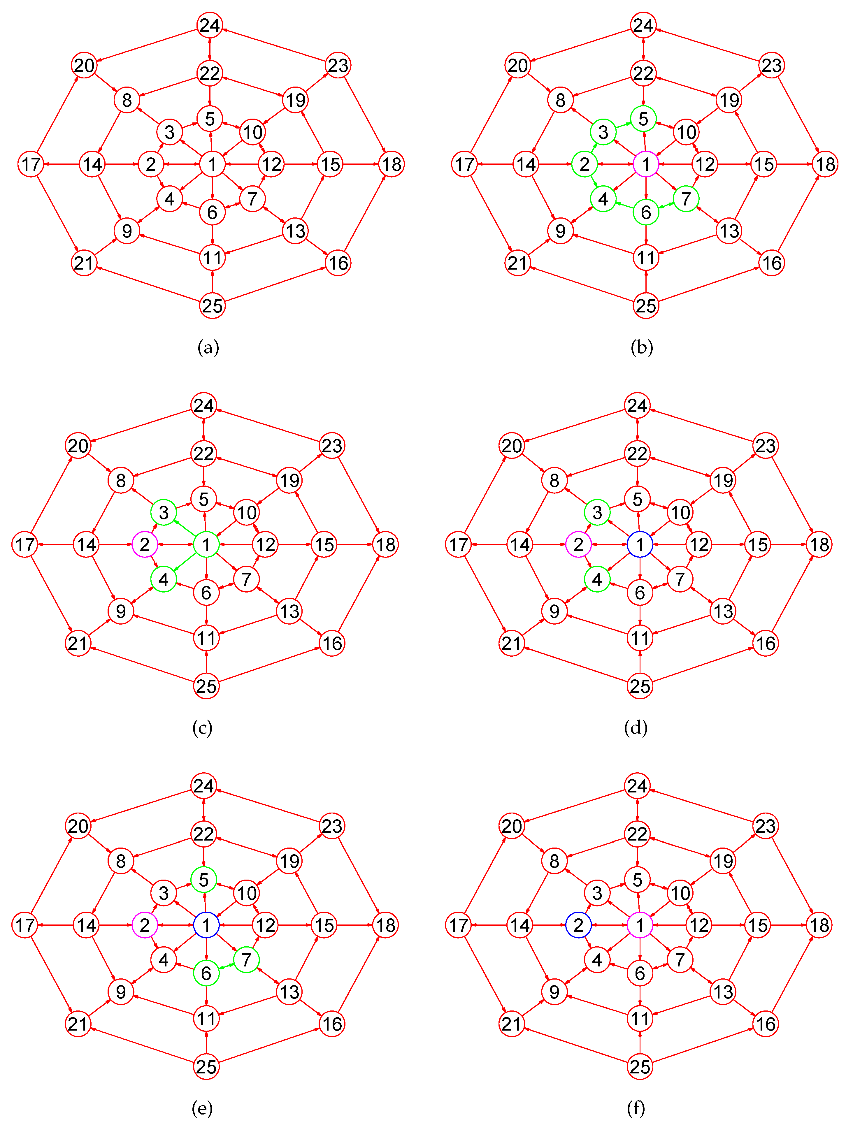
Definition 9.

Let $G=<V(G)$, $E(G)>$ be a simple digraph with n nodes. The open neighborhood, in-neighborhood, out-neighborhood, outin-neighborhood, and mix-neighborhood subdigraphs of a vertex u in G are subdigraphs of G defined as

$$\begin{array}{cccccccccccccccccccc}& N\hfill & & (u)=(V(N\hfill & & (u)),\hfill & & E(N\hfill & & (u))),\hfill & & N^{-}& & (u)=(V(N^{-}& & (u))& & ,E(N^{-}& & (u))),\\ & N^{+}\hfill & & (u)=(V(N^{+}\hfill & & (u)),\hfill & & E(N^{+}\hfill & & (u))),\hfill & & N^{+-}& & (u)=(V(N^{+-}& & (u))& & ,E(N^{+-}& & (u))),\\ & N^{++}\hfill & & (u)=(V(N^{++}\hfill & & (u)),\hfill & & E(N^{++}\hfill & & (u)))\hfill & & & & & & & & & & \end{array}$$

(8)

where

$$\begin{array}{cccccccc}& V(N\hfill & & (u))\hfill & & =\{v\in V(G)-u\hfill & & |v\to u\in E(G)\vee u\to v\in E(G)\},\hfill \\ & E(N\hfill & & (u))\hfill & & =\{v\to w\in E(G)\hfill & & |v,w\in V(N(u))\},\hfill \end{array}$$

(9)

$$\begin{array}{cccccccc}& V(N^{-}\hfill & & (u))\hfill & & =\{v\in V(G)-u\hfill & & |v\to u\in E(G)\wedge u\to v\notin E(G)\},\hfill \\ & E(N^{-}\hfill & & (u))\hfill & & =\{v\to w\in E(G)\hfill & & |v,w\in V(N^{-}(u))\},\hfill \end{array}$$

(10)

$$\begin{array}{cccccccc}& V(N^{+}\hfill & & (u))\hfill & & =\{v\in V(G)-u\hfill & & |u\to v\in E(G)\wedge v\to u\notin E(G)\},\hfill \\ & E(N^{+}\hfill & & (u))\hfill & & =\{v\to w\in E(G)\hfill & & |v,w\in V(N^{+}(u))\},\hfill \end{array}$$

(11)

$$\begin{array}{cccccccc}& V(N^{+-}\hfill & & (u))\hfill & & =\{v\in V(G)-u\hfill & & |u\to v\in E(G)\wedge v\to u\in E(G)\},\hfill \\ & E(N^{+-}\hfill & & (u))\hfill & & =\{v\to w\in E(G)\hfill & & |v,w\in V(N^{+-}(u))\}.\hfill \end{array}$$

(12)

$$\begin{array}{cccccccc}& V(N^{++}\hfill & & (u))\hfill & & =V(N^{+-}(u))\cup V(\hfill & & N^{+}(u)),\hfill \\ & E(N^{++}\hfill & & (u))\hfill & & =\{v\to w\in E(G)\hfill & & |v,w\in V(N^{++}(u))\}.\hfill \end{array}$$

(13)

The open k-neighborhood, k-in-neighborhood, k-out-neighborhood, k-outin-neighborhood, and k-mix-neighborhood subdigraphs of u with k ⩾ 2 are subdigraphs of G defined as

$$\begin{array}{cccccccccccccccccccccc}& N_k\hfill & & (u)=(V(N_k\hfill & & (u))\hfill & & ,E(N_k\hfill & & (u))),\hfill & & N_k^{-}& & (u)& & =(V(N_k^{-}& & (u)),& & E(N_k^{-}& & (u))),\\ & N_k^{+}\hfill & & (u)=(V(N_k^{+}\hfill & & (u))\hfill & & ,E(N_k^{+}\hfill & & (u))),\hfill & & N_k^{+-}& & (u)& & =(V(N_k^{+-}& & (u)),& & E(N_k^{+-}& & (u))),\\ & N_k^{++}\hfill & & (u)=(V(N_k^{++}\hfill & & (u))\hfill & & ,E(N_k^{++}\hfill & & (u)))\hfill & & & & & & & & & & & \end{array}$$

where

$$\begin{array}{cccccccc}& V(N_k\hfill & & (u))\hfill & & =\{v\in V(G)-u\hfill & & |d(u,v)⩽k\vee d(v,u)⩽k\},\hfill \\ & E(N_k\hfill & & (u))\hfill & & =\{v\to w\in E(G)\hfill & & |v,w\in V(N_k(u))\},\hfill \end{array}$$

(14)

$$\begin{array}{cccccccc}& V(N_k^{-}\hfill & & (u))\hfill & & =\{v\in V(G)-u\hfill & & |d(v,u)⩽k\},\hfill \\ & E(N_k^{-}\hfill & & (u))\hfill & & =\{v\to w\in E(G)\hfill & & |v,w\in V(N_k^{-}(u))\},\hfill \end{array}$$

(15)

$$\begin{array}{cccccccc}& V(N_k^{+}\hfill & & (u))\hfill & & =\{v\in V(G)-u\hfill & & |d(u,v)⩽k\},\hfill \\ & E(N_k^{+}\hfill & & (u))\hfill & & =\{v\to w\in E(G)\hfill & & |v,w\in V(N_k^{+}(u))\},\hfill \end{array}$$

(16)

$$\begin{array}{cccccccc}& V(N_k^{+-}\hfill & & (u))\hfill & & =\{v\in V(G)-u\hfill & & |d(u,v)=d(v,u)⩽k\},\hfill \\ & E(N_k^{+-}\hfill & & (u))\hfill & & =\{v\to w\in E(G)\hfill & & |v,w\in V(N_k^{+-}(u))\}.\hfill \end{array}$$

(17)

$$\begin{array}{cccccccc}& V(N_k^{++}\hfill & & (u))\hfill & & =V(N_k^{+-}(u))\cup V(N\hfill & & {}_k^{+}(u)),\hfill \\ & E(N_k^{++}\hfill & & (u))\hfill & & =\{v\to w\in E(G)\hfill & & |v,w\in V(N_k^{++}(u))\}.\hfill \end{array}$$

(18)

Definition 10.

Let $G=<V(G)$, $E(G)>$ be a simple digraph with n nodes. The close neighborhood, in-neighborhood, out-neighborhood, outin-neighborhood, and mix-neighborhood subdigraphs of a vertex u in G are subdigraphs of G defined as

$$\begin{array}{cccccccccccccccccccc}& N\hfill & & [u]=(V(N\hfill & & [u]),\hfill & & E(N\hfill & & [u])),\hfill & & N^{-}& & [u]=(V(N^{-}& & [u])& & ,E(N^{-}& & [u])),\\ & N^{+}\hfill & & [u]=(V(N^{+}\hfill & & [u]),\hfill & & E(N^{+}\hfill & & [u])),\hfill & & N^{+-}& & [u]=(V(N^{+-}& & [u])& & ,E(N^{+-}& & [u])),\\ & N^{++}\hfill & & [u]=(V(N^{++}\hfill & & [u]),\hfill & & E(N^{++}\hfill & & [u]))\hfill & & & & & & & & & \end{array}$$

where

$$\begin{array}{cccccccccccc}& V(N\hfill & & [u])=V(N\hfill & & (u))\cup \{u\},\hfill & & E(N\hfill & & [u])=\{v\to w\in E(G)|v,w\in V(N\hfill & & [u])\},\end{array}$$

(19)

$$\begin{array}{cccccccccccc}& V(N^{-}\hfill & & [u])=V(N^{-}\hfill & & (u))\cup \{u\},\hfill & & E(N^{-}\hfill & & [u])=\{v\to w\in E(G)|v,w\in V(N^{-}\hfill & & [u])\},\end{array}$$

(20)

$$\begin{array}{cccccccccccc}& V(N^{+}\hfill & & [u])=V(N^{+}\hfill & & (u))\cup \{u\},\hfill & & E(N^{+}\hfill & & [u])=\{v\to w\in E(G)|v,w\in V(N^{+}\hfill & & [u])\},\end{array}$$

(21)

$$\begin{array}{cccccccccccc}& V(N^{+-}\hfill & & [u])=V(N^{+-}\hfill & & (u))\cup \{u\},\hfill & & E(N^{+-}\hfill & & [u])=\{v\to w\in E(G)|v,w\in V(N^{+-}\hfill & & [u])\},\end{array}$$

(22)

$$\begin{array}{cccccccccccc}& V(N^{++}\hfill & & [u])=V(N^{+-}\hfill & & [u])\cup V(N^{+}[u]),\hfill & & E(N^{++}\hfill & & [u])=\{v\to w\in E(G)|v,w\in V(N^{++}\hfill & & [u])\}.\end{array}$$

(23)

The close k-neighborhood, k-in-neighborhood, k-out-neighborhood, k-outin-neighborhood, and k-mix-neighborhood subdigraphs of u with k ⩾ 2 are subdigraphs of G defined as

$$\begin{array}{cccccccccccccccccccc}& N_k\hfill & & [u]=(V(N_k\hfill & & [u]),\hfill & & E(N_k\hfill & & [u])),\hfill & & N_k^{-}& & [u]=(V(N_k^{-}& & [u]),& & E(N_k^{-}& & [u])),\\ & N_k^{+}\hfill & & [u]=(V(N_k^{+}\hfill & & [u]),\hfill & & E(N_k^{+}\hfill & & [u])),\hfill & & N_k^{+-}& & [u]=(V(N_k^{+-}& & [u]),& & E(N_k^{+-}& & [u])),\\ & N_k^{++}\hfill & & [u]=(V(N_k^{++}\hfill & & [u]),\hfill & & E(N_k^{++}\hfill & & [u]))\hfill & & & & & & & & & & \end{array}$$

where

$$\begin{array}{cccccccccccc}& V(N_k\hfill & & [u])=V(N_k\hfill & & (u))\cup \{u\},\hfill & & E(N_k\hfill & & [u])=\{v\to w\in E(G)|v,w\in V(N_k\hfill & & [u])\},\end{array}$$

(24)

$$\begin{array}{cccccccccccc}& V(N_k^{-}\hfill & & [u])=V(N_k^{-}\hfill & & (u))\cup \{u\},\hfill & & E(N_k^{-}\hfill & & [u])=\{v\to w\in E(G)|v,w\in V(N_k^{-}\hfill & & [u])\},\end{array}$$

(25)

$$\begin{array}{cccccccccccc}& V(N_k^{+}\hfill & & [u])=V(N_k^{+}\hfill & & (u))\cup \{u\},\hfill & & E(N_k^{-}\hfill & & [u])=\{v\to w\in E(G)|v,w\in V(N_k^{+}\hfill & & [u])\},\end{array}$$

(26)

$$\begin{array}{cccccccccccc}& V(N_k^{+-}\hfill & & [u])=V(N_k^{+-}\hfill & & (u))\cup \{u\},\hfill & & E(N_k^{+-}\hfill & & [u])=\{v\to w\in E(G)|v,w\in V(N_k^{+-}\hfill & & [u])\},\end{array}$$

(27)

$$\begin{array}{cccccccccccc}& V(N_k^{++}\hfill & & [u])=V(N_k^{+-}\hfill & & [u])\cup V(N_k^{+}[u]),\hfill & & E(N_k^{++}\hfill & & [u])=\{v\to w\in E(G)|v,w\in V(N_k^{++}\hfill & & [u])\}.\end{array}$$

(28)

Definition 11.

Let $G=<V(G)$, $E(G)>$ be a simple digraph with n nodes. The open neighborhood, in-neighborhood, out-neighborhood, outin-neighborhood, and mix-neighborhood subdigraphs of a nodes set $Q\subseteq V(G)$ are subdigraphs of G defined as

$$\begin{array}{cccccccccccccccccccc}& N\hfill & & (Q)=(V(N\hfill & & (Q))\hfill & & ,E(N\hfill & & (Q))),\hfill & & N^{-}& & (Q)=(V(N^{-}& & (Q))& & ,E(N^{-}& & (Q))),\\ & N^{+}\hfill & & (Q)=(V(N^{+}\hfill & & (Q))\hfill & & ,E(N^{+}\hfill & & (Q))),\hfill & & N^{+-}& & (Q)=(V(N^{+-}& & (Q))& & ,E(N^{+-}& & (Q))),\\ & N^{++}\hfill & & (Q)=(V(N^{++}\hfill & & (Q))\hfill & & ,E(N^{++}\hfill & & (Q)))\hfill & & & & & & & & & \end{array}$$

where

$$\begin{array}{cccccccc}& V(N\hfill & & (Q))\hfill & & =\{v\in V(G)-Q\hfill & & |\exists u\in Q\wedge (v\to u\in E(G)\vee u\to v\in E(G))\},\hfill \\ & E(N\hfill & & (Q))\hfill & & =\{v\to w\in E(G)\hfill & & |v,w\in V(N(Q))\},\hfill \end{array}$$

(29)

$$\begin{array}{cccccccc}& V(N^{-}\hfill & & (Q))\hfill & & =\{v\in V(G)-Q\hfill & & |\exists u\in Q\wedge v\to u\in E(G)\wedge u\to v\notin E(G)\},\hfill \\ & E(N^{-}\hfill & & (Q))\hfill & & =\{v\to w\in E(G)\hfill & & |v,w\in V(N^{-}(Q))\},\hfill \end{array}$$

(30)

$$\begin{array}{cccccccc}& V(N^{+}\hfill & & (Q))\hfill & & =\{v\in V(G)-Q\hfill & & |\exists u\in Q\wedge u\to v\in E(G)\wedge v\to u\notin E(G)\},\hfill \\ & E(N^{+}\hfill & & (Q))\hfill & & =\{v\to w\in E(G)\hfill & & |v,w\in V(N^{+}(Q))\},\hfill \end{array}$$

(31)

$$\begin{array}{cccccccc}& V(N^{+-}\hfill & & (Q))\hfill & & =\{v\in V(G)-Q\hfill & & |\exists u\in Q\wedge u\to v\in E(G)\wedge v\to u\in E(G)\},\hfill \\ & E(N^{-+}\hfill & & (Q))\hfill & & =\{v\to w\in E(G)\hfill & & |v,w\in V(N^{+-}(Q))\},\hfill \end{array}$$

(32)

$$\begin{array}{cccccccccc}& V(N^{++}\hfill & & (Q))\hfill & & =V(N^{+-}(Q))\cup V(\hfill & & N^{+}(Q)),\hfill & & \hfill \\ & E(N^{++}\hfill & & (Q))\hfill & & =\{v\to w\in E(G)\hfill & & |v,w\in V(N^{++}(Q))\}.\hfill \end{array}$$

(33)

The open k-neighborhood, k-in-neighborhood, k-out-neighborhood, k-outin-neighborhood, and k-mix-neighborhood subdigraphs of Q with k ⩾ 2 are subdigraphs of G defined as

$$\begin{array}{cccccccccccccccccccc}& N_k\hfill & & (Q)=(V(N_k\hfill & & (Q))\hfill & & ,E(N_k\hfill & & (Q))),\hfill & & N_k^{-}& & (Q)=(V(N_k^{-}& & (Q))& & ,E(N_k^{-}& & (Q))),\\ & N_k^{+}\hfill & & (Q)=(V(N_k^{+}\hfill & & (Q))\hfill & & ,E(N_k^{+}\hfill & & (Q))),\hfill & & N_k^{+-}& & (Q)=(V(N_k^{+-}& & (Q))& & ,E(N_k^{+-}& & (Q))),\\ & N_k^{++}\hfill & & (Q)=(V(N_k^{++}\hfill & & (Q))\hfill & & ,E(N_k^{++}\hfill & & (Q)))\hfill & & & & & & & & & \end{array}$$

where

$$\begin{array}{cccccccc}& V(N_k\hfill & & (Q))\hfill & & =\{v\in V(G)-Q\hfill & & |\exists u\in Q\wedge (d(v,u)⩽k\vee d(u,v)⩽k)\},\hfill \\ & E(N_k\hfill & & (Q))\hfill & & =\{v\to w\in E(G)\hfill & & |v,w\in V(N_k(Q))\},\hfill \end{array}$$

(34)

$$\begin{array}{cccccccc}& V(N_k^{-}\hfill & & (Q))\hfill & & =\{v\in V(G)-Q\hfill & & |\exists u\in Q\wedge d(v,u)⩽k\},\hfill \\ & E(N_k^{-}\hfill & & (Q))\hfill & & =\{v\to w\in E(G)\hfill & & |v,w\in V(N_k^{-}(Q))\},\hfill \end{array}$$

(35)

$$\begin{array}{cccccccc}& V(N_k^{+}\hfill & & (Q))\hfill & & =\{v\in V(G)-Q\hfill & & |\exists u\in Q\wedge d(u,v)⩽k\},\hfill \\ & E(N_k^{+}\hfill & & (Q))\hfill & & =\{v\to w\in E(G)\hfill & & |v,w\in V(N_k^{+}(Q))\},\hfill \end{array}$$

(36)

$$\begin{array}{cccccccc}& V(N_k^{+-}\hfill & & (Q))\hfill & & =\{v\in V(G)-Q\hfill & & |\exists u\in Q\wedge d(u,v)=d(v,u)⩽k\},\hfill \\ & E(N_k^{+-}\hfill & & (Q))\hfill & & =\{v\to w\in E(G)\hfill & & |v,w\in V(N_k^{+-}(Q))\},\hfill \end{array}$$

(37)

$$\begin{array}{cccccccc}& V(N_k^{++}\hfill & & (Q))\hfill & & =V(N_k^{+-}(Q))\cup V(\hfill & & N_k^{+}(Q)),\hfill \\ & E(N_k^{++}\hfill & & (Q))\hfill & & =\{v\to w\in E(G)\hfill & & |v,w\in V(N_k^{++}(Q))\}.\hfill \end{array}$$

(38)

Definition 12.

Let $G=<V(G)$, $E(G)>$ be a simple digraph with n nodes. The close neighborhood, in-neighborhood, out-neighborhood, outin-neighborhood, and mix-neighborhood subdigraphs of a nodes set $Q\subseteq V(G)$ are subdigraphs of G defined as

$$\begin{array}{cccccccccccccccccccc}& N\hfill & & [Q]=(V(N\hfill & & [Q])\hfill & & ,E(N\hfill & & [Q])),\hfill & & N^{-}& & [Q]=(V(N^{-}& & [Q])& & ,E(N^{-}& & [Q])),\\ & N^{+}\hfill & & [Q]=(V(N^{+}\hfill & & [Q])\hfill & & ,E(N^{+}\hfill & & [Q])),\hfill & & N^{+-}& & [Q]=(V(N^{+-}& & [Q])& & ,E(N^{+-}& & [Q])),\\ & N^{++}\hfill & & [Q]=(V(N^{++}\hfill & & [Q])\hfill & & ,E(N^{++}\hfill & & [Q]))\hfill & & & & & & & & & \end{array}$$

where

$$\begin{array}{cccccccccccc}& V(N\hfill & & [Q])=V(N\hfill & & (Q))\cup Q,\hfill & & E(N\hfill & & [Q])=\{v\to w\in E(G)|v,w\in V(N\hfill & & [Q])\},\end{array}$$

(39)

$$\begin{array}{cccccccccccc}& V(N^{-}\hfill & & [Q])=V(N^{-}\hfill & & (Q))\cup Q,\hfill & & E(N^{-}\hfill & & [Q])=\{v\to w\in E(G)|v,w\in V(N^{-}\hfill & & [Q])\},\end{array}$$

(40)

$$\begin{array}{cccccccccccc}& V(N^{+}\hfill & & [Q])=V(N^{+}\hfill & & (Q))\cup Q,\hfill & & E(N^{+}\hfill & & [Q])=\{v\to w\in E(G)|v,w\in V(N^{+}\hfill & & [Q])\},\end{array}$$

(41)

$$\begin{array}{cccccccccccc}& V(N^{+-}\hfill & & [Q])=V(N^{+-}\hfill & & (Q))\cup Q,\hfill & & E(N^{+-}\hfill & & [Q])=\{v\to w\in E(G)|v,w\in V(N^{+-}\hfill & & [Q])\},\end{array}$$

(42)

$$\begin{array}{cccccccccccc}& V(N^{++}\hfill & & [Q])=V(N^{+-}\hfill & & [Q])\cup V(N^{+}[Q]),\hfill & & E(N^{++}\hfill & & [Q])=\{v\to w\in E(G)|v,w\in V(N^{++}\hfill & & [Q])\}.\end{array}$$

(43)

The close k-neighborhood, k-in-neighborhood, k-out-neighborhood, k-outin-neighborhood, and k-mix-neighborhood subdigraphs of Q with k ⩾ 2 are subdigraphs of G defined as

$$\begin{array}{cccccccccccccccccccc}& N_k\hfill & & [Q]=(V(N_k\hfill & & [Q]),\hfill & & E(N_k\hfill & & [Q])),\hfill & & N_k^{-}& & [Q]=(V(N_k^{-}& & [Q]),& & E(N_k^{-}& & [Q])),\\ & N_k^{+}\hfill & & [Q]=(V(N_k^{+}\hfill & & [Q]),\hfill & & E(N_k^{+}\hfill & & [Q])),\hfill & & N_k^{+-}& & [Q]=(V(N_k^{+-}& & [Q]),& & E(N_k^{+-}& & [Q])),\\ & N_k^{++}\hfill & & [Q]=(V(N_k^{++}\hfill & & [Q]),\hfill & & E(N_k^{++}\hfill & & [Q]))\hfill & & & & & & & & & \end{array}$$

where

$$\begin{array}{cccccccccccc}& V(N_k\hfill & & [Q])=V(N_k\hfill & & (Q))\cup Q,\hfill & & E(N_k\hfill & & [Q])=\{v\to w\in E(G)|v,w\in V(N_k\hfill & & [Q])\},\end{array}$$

(44)

$$\begin{array}{cccccccccccc}& V(N_k^{-}\hfill & & [Q])=V(N_k^{-}\hfill & & (Q))\cup Q,\hfill & & E(N_k^{-}\hfill & & [Q])=\{v\to w\in E(G)|v,w\in V(N_k^{-}\hfill & & [Q])\},\end{array}$$

(45)

$$\begin{array}{cccccccccccc}& V(N_k^{+}\hfill & & [Q])=V(N_k^{+}\hfill & & (Q))\cup Q,\hfill & & E(N_k^{+}\hfill & & [Q])=\{v\to w\in E(G)|v,w\in V(N_k^{+}\hfill & & [Q])\},\end{array}$$

(46)

$$\begin{array}{cccccccccccc}& V(N_k^{+-}\hfill & & [Q])=V(N_k^{+-}\hfill & & (Q))\cup Q,\hfill & & E(N_k^{+-}\hfill & & [Q])=\{v\to w\in E(G)|v,w\in V(N_k^{+-}\hfill & & [Q])\},\end{array}$$

(47)

$$\begin{array}{cccccccccccc}& V(N_k^{++}\hfill & & [Q])=V(N_k^{+-}\hfill & & [Q])\cup V(N_k^{+}[Q]),\hfill & & E(N_k^{++}\hfill & & [Q])=\{v\to w\in E(G)|v,w\in V(N_k^{++}\hfill & & [Q])\}.\end{array}$$

(48)

In the following section, unless otherwise specified, each k-neighborhood, k-in-neighborhood, k-out-neighborhood, k-outin-neighborhood, and k-mix-neighborhood subdigraphs are closed.

A digraph is connected if its underlying graph is connected. For $k=1$, we omit the subscript 1 and let $N^{++}(u)=N_1^{++}(u)$, $N^{++}[u]=N_1^{++}[u]$, $N^{++}(Q)=N_1^{++}(Q)$, and $N^{++}[Q]=N_1^{++}[Q]$.

Definition 13.

Let $G=<V(G)$, $E(G)>$ be a simple digraph with n nodes. Suppose that $H\subseteq G$ and $u\in V(H)$. We denote by $N_H^k(u)$ the open k-neighborhood subdigraph of u in H, by $N_H^k[u]$ the close k − neighborhood subdigraph of u in H, by $N_H^{k++}(u)$ the open k-mix-neighborhood subdigraph of u in H, and by $N_H^{k++}[u]$ the close k-mix-neighborhood subdigraph of u in H.

For $k=1$, we omit the superscript 1 and let $N_H(u)=N_H^1(u)$, $N_H[u]=N_H^1[u]$, $N_H^{++}(u)=N_H^{1++}(u)$, and $N_H^{++}[u]=N_H^{1++}[u]$.

Definition 14.

Let $G=<V(G)$, $E(G)>$ be a simple connected digraph with n nodes. For every $u\in V(G)$, there exists a positive integer k satisfying conditions $N_{k-1}[u]\subset G$ and $N_k[u]=G$. The value of k is called the diffusion radius of u denoted by of u denoted by ${\rho }_G[u]$, and the subscript G can be omitted when no ambiguity can arise.

By Definition 14, it is clear that $N_{\rho [u]}[u]=G$ for every u in G.

Definition 15.

Let $G=<V(G)$, $E(G)>$ be a simple connected digraph with n nodes. For every $u\in V(G)$, there exists a positive integer k satisfying conditions $N_{k-1}^{++}[u]\subset G$ and $N_k^{++}[u]=N_{k-1}^{++}[u]$. The value of k is called the mix diffusion radius of u denoted by of u denoted by ${\rho }_G^{++}[u]$, and the subscript G can be omitted when no ambiguity can arise.

Definition 16.

Let $G=<V(G)$, $E(G)>$ be a simple digraph and u be a node in G whose close k neighborhood subdigraph is $N_k[u]$ with $k=1,2,\cdots$. A node in $N[u]$ is a one diffusion node of u. For $k>1$, a node v in $N_k[u]$ satisfying condition $v\notin N_{k-1}[u]$ is a k diffusion node of u.

Definition 17.

Let $G=<V(G)$, $E(G)>$ be a simple digraph and u be a node in G whose close k-mix-neighborhood subdigraph is $N_k^{++}[u]$ with $k=1,2,\cdots$. A node in $N^{++}[u]$ is a one mix diffusion node of u. For $k>1$, a node v in $N_k^{++}[u]$ satisfying condition $v\notin N_{k-1}^{++}[u]$ is a k mix diffusion node of u.

Every node v in G is assigned an attribute m_NearestNode whose function, described in Section 3.1.2.

Definition 18.

Let $G=<V(G)$, $E(G)>$ be a simple digraph and u be a node in G whose close k neighborhood subdigraph is $N_k[u]$ with $k=1,2,\cdots$. Assume that H is a connected component of $N_k[u]$ with $k⩾1$. Assume that $V_m\subseteq V(H)$ with $m=0,1,2,\cdots ,t$, where $V_0$ is in ascending order of attribute $m\_NearestNode$ with $v->m\_NearestNode⩾1$ for every $v\in V_0$, and $V_1,V_2$, $\cdots ,V_t$ contain the $1,2,\cdots ,k$ diffusion nodes of u respectively, satisfying conditions $V_0\cup V_1\cup \cdots \cup V_t=V(H)$ and $V_i\cap V_j=\varnothing$ for $i\ne j,i,j=0,1,\cdots ,t$.

We define $d_{\sigma }^{+}(H)=(d_{N_k[u]}^{+}(V_0)$, ⋯, $d_{N_k[u]}^{+}(V_i)$, ⋯, $d_{N_k[u]}^{+}(V_t))$ to be the diffusion outdegree sequence of H where $d_{N_k[u]}^{+}(V_i)$ with $i=0,1,\cdots ,t$ are the outdegree sequences in descending order induced by all vertices in $V_i$ respectively.

Definition 19.

Let $G=<V(G)$, $E(G)>$ be a simple digraph and u be a node in G whose close k-mix-neighborhood subdigraph is $N_k^{++}[u]$ with $k=1,2,\cdots$. Assume that H is a connected component of $N_k^{++}[u]$ with $k⩾1$. Assume that $V_m\subseteq V(H)$ with $m=0,1,2,\cdots ,t$, where $V_0$ is in ascending order of attribute $m\_NearestNode$ with $v->m\_NearestNode⩾1$ for every $v\in V_0$, and $V_1,V_2$, $\cdots ,V_t$ contain the $1,2,\cdots ,k$ mix diffusion nodes of u respectively, satisfying conditions $V_0\cup V_1\cup \cdots \cup V_t=V(H)$ and $V_i\cap V_j=\varnothing$ for $i\ne j,i,j=0,1,\cdots ,t$.

We define $d_{\tau }^{+}(H)=(d_{N_k^{++}[u]}^{+}(V_0)$, ⋯, $d_{N_k^{++}[u]}^{+}(V_i)$, ⋯, $d_{N_k^{++}[u]}^{+}(V_t))$ to be the mix diffusion outdegree sequence of H where $d_{N_k^{++}[u]}^{+}(V_i)$ with $i=0,1,\cdots ,t$ are the outdegree sequences in descending order induced by all vertices in $V_i$ respectively.

Definition 20.

Let $G=<V(G)$, $E(G)>$ be a simple digraph and u be a node in G whose close k neighborhood subdigraph is $N_k[u]$ with $k=1,2,\cdots$. Assume that $N_k[u]$ has p connected components $H_1$, $H_2$, ⋯, $H_p$ with diffusion outdegree sequences $d_{\sigma }^{+}(H_1)$, $d_{\sigma }^{+}(H_2)$, ⋯, $d_{\sigma }^{+}(H_p)$ respectively, satisfying conditions $d_{\sigma }^{+}(H_1)⩾d_{\sigma }^{+}(H_2)⩾\cdots ⩾d_{\sigma }^{+}(H_p)$.

Define $d_G^{\sigma }[N_k(u)]=(d_{\sigma }(H_1)$, $d_{\sigma }(H_2)$, ⋯, $d_{\sigma }(H_p))$ to be the entire mix diffusion outdegree sequence of $N_k(u)$ pertaining to u in G, and omit the subscript G when no ambiguity can arise.

Definition 21.

Let $G=<V(G)$, $E(G)>$ be a simple digraph and u be a node in G whose close k-mix neighborhood subdigraph is $N_k^{++}[u]$ with $k=1,2,\cdots$. Assume that $N_k^{++}[u]$ has p connected components $H_1$, $H_2$, ⋯, $H_p$ with mix diffusion outdegree sequences $d_{\tau }^{+}(H_1)$, $d_{\tau }^{+}(H_2)$, ⋯, $d_{\tau }^{+}(H_p)$ respectively, satisfying conditions $d_{\tau }^{+}(H_1)⩾d_{\tau }^{+}(H_2)⩾\cdots ⩾d_{\tau }^{+}(H_p)$.

Define $d_G^{\tau }[N_k^{++}[u]]=(d_{\tau }^{+}(H_1)$, $d_{\sigma }^{+}(H_2)$, ⋯, $d_{\tau }^{+}(H_p))$ to be the entire mix diffusion outdegree sequence of $N_k^{++}[u]$ pertaining to u in G, and omit the subscript G when no ambiguity can arise.

Definition 22.

Let $G=<V(G)$, $E(G)>$ be a simple digraph with n nodes. For every $u,v\in V(G)$ with $u\ne v$ and , let $N_1^{++}[u]$, $N_2^{++}[u]$, ⋯, $N_{{\rho }^{++}[u]}^{++}[u]$ be the close 1, 2, ⋯, ${\rho }^{++}[u]$ mix-neighborhood subdigraph of u with entire mix diffusion outdegree sequences $d^{\tau }[N_1^{++}[u]]$, $d^{\tau }[N_2^{++}[u]]$, ⋯, $d^{\tau }[N_{{\rho }^{++}[u]}^{++}[u]]$, respectively. Let $N_1^{++}[v]$, $N_2^{++}[v]$, ⋯, $N_{{\rho }^{++}[v]}^{++}[v]$ be the 1, 2, ⋯, ${\rho }^{++}[v]$ mix-neighborhood subdigraph of v with entire mix diffusion outdegree sequences $d^{\tau }[N_1^{++}[v]]$, $d^{\tau }[N_2^{++}[v]]$, ⋯, $d^{\tau }[N_{{\rho }^{++}[v]}^{++}[v]]$, respectively. Let $Z_1=(d^{\tau }[N_1^{++}[u]]$, $d^{\tau }[N_2^{++}[u]]$, ⋯, $d^{\tau }[N_{{\rho }^{++}[u]}^{++}[u]])$ and $Z_2=(d^{\tau }[N_1^{++}[v]]$, $d^{\tau }[N_2^{++}[v]]$, ⋯, $d^{\tau }[N_{{\rho }^{++}[v]}^{++}[v]])$. If $Z_1>Z_2$, we write $u\succ v$ with respect to G. Otherwise, if $Z_1<Z_2$, we write $u\prec v$ with respect to G. Otherwise, if $Z_1=Z_2$, we write $u\asymp v$ with respect to G, and omit the symbol G when no ambiguity can arise. Denote $u\succ v$ or $u\asymp v$ by $u\succcurlyeq v$ and $u\prec v$ or $u\asymp v$ by $u\preccurlyeq v$.

It is clear that ≻, ≺, ≍, ≽ define a binary relation on the set of nodes $V(G)$. By Definition 22, for every $u,v\in V(G)$ with $u\ne v$, one of the following statements is true: (1) $u\succ v$. (2) $u\prec v$. (3) $u\asymp v$.

It can be shown that $(V(G)$, $\succcurlyeq )$ is a well-ordered set, where ≽ denotes the binary relation $u\succcurlyeq v$ on the set $V(G)$. By the well-ordering theorem, it follows that there exists a maximum and minimum element in $V(G)$, denoted by $G_{max}^{\succcurlyeq }$ and $G_{min}^{\succcurlyeq }$ respectively with $G_{max}^{\succcurlyeq }\in V(G)$ and $G_{min}^{\succcurlyeq }\in V(G)$. The symbol ≽ can be omitted if no confusion arises. The following Lemmas 2–4 immediately follow from Definition 22.

Lemma 2.

Let $G=<V(G)$, $E(G)>$ be a simple digraph with n nodes. For every $u,v\in V(G)$ with $u\ne v$, if the symbol ≽ denotes the binary relation $u\succcurlyeq v$ on the set $V(G)$, then, all of the nodes in G form a single chain L on G: $v_1\succcurlyeq v_2\succcurlyeq \cdots \succcurlyeq v_i\succcurlyeq \cdots \succcurlyeq v_n$ with $v_i\in V(G)$, $i=1,2$, $\cdots ,n$.

Lemma 3.

Let $G=<V(G)$, $E(G)>$ be a simple digraph with n nodes. Let $S^{+}(G)=\{u\in V(G)|d^{+}(u)={\Delta }^{+}(G)=s\}$. For every $u,v\in S^{+}(G)$ with $u\ne v$, if the symbol ≽ denotes the binary relation $u\succcurlyeq v$ on the set $S^{+}(G)$, then, all of the nodes in $S^{+}(G)$ form a single chain L on G: $v_1\succcurlyeq v_2\succcurlyeq \cdots \succcurlyeq v_i\succcurlyeq \cdots \succcurlyeq v_s$ with $v_i\in S^{+}(G),i=1,2,\cdots ,s$.

Lemma 4.

Let $G=<V(G)$, $E(G)>$ be a simple digraph with n nodes. For every $u\in V(G)$, suppose that $N_k^{++}[u]$ is the close k mix-neighborhood subdigraph of u in G. Let $S^{+}(N_k^{++}[u])=\{v\in V(N_k^{++}[u])|d^{+}(v)={\Delta }^{+}(N_k^{++}[u])=t\}$.

For every $v,w\in S^{+}(N_k^{++}[u])$ with $v\ne w$, if the symbol ≽ denotes the binary relation $v\succcurlyeq w$ on the set $S^{+}(N_k^{++}[u])$, then, all of the nodes in $S^{+}(N_k^{++}[u])$ form a single chain L on $N_k^{++}[u]$: $v_1\succcurlyeq v_2\succcurlyeq \cdots \succcurlyeq v_i\succcurlyeq \cdots \succcurlyeq v_t$ with $v_i\in S^{+}(N_k^{++}[u]),i=1,2,\cdots ,t$.

The conclusions in the following Propositions 1 and 2 are obvious by Definitions 4, 5, and 22.

Proposition 1.

Let $G=<V(G)$, $E(G)>$ be a simple digraph with n nodes. For every $u,v\in V(G)$ with $u\ne v$ and , let $N_1^{++}[u]$, $N_2^{++}[u]$, ⋯, $N_{{\rho }^{++}[u]}^{++}[u]$ be the close 1, 2, ⋯, ${\rho }^{++}[u]$ mix-neighborhood subdigraph of u with entire mix diffusion outdegree sequences $d^{\tau }[N_1^{++}[u]]$, $d^{\tau }[N_2^{++}[u]]$, ⋯, $d^{\tau }[N_{{\rho }^{++}[u]}^{++}[u]]$, respectively. Let $N_1^{++}[v]$, $N_2^{++}[v]$, ⋯, $N_{{\rho }^{++}[v]}^{++}[v]$ be the close 1, 2, ⋯, ${\rho }^{++}[v]$ mix-neighborhood subdigraph of v with entire mix diffusion outdegree sequences $d^{\tau }[N_1^{++}[v]]$, $d^{\tau }[N_2^{++}[v]]$, ⋯, $d^{\tau }[N_{{\rho }^{++}[v]}^{++}[v]]$, respectively. Let $Z_1=(d^{\tau }[N_1^{++}[u]]$, $d^{\tau }[N_2^{++}[u]]$, ⋯, $d^{\tau }[N_{{\rho }^{++}[u]}^{++}[u]])=(X_1,Y_1)$ with $X_1=(d^{\tau }[N_1^{++}[u]]$, $d^{\tau }[N_2^{++}[u]]$, ⋯, $d^{\tau }[N_k^{++}[u]])$ and $Y_1=(d^{\tau }[N_{k+1}^{++}[u]]$, $d^{\tau }[N_{k+2}^{++}[u]]$, ⋯, $d^{\tau }[N_{{\rho }^{++}[u]}^{++}[u]])$. Let $Z_2=(d^{\tau }[N_1^{++}[v]]$, $d^{\tau }[N_2^{++}[v]]$, ⋯, $d^{\tau }[N_{{\rho }^{++}[v]}^{++}[v]])=(X_2,Y_2)$ with $X_2=(d^{\tau }[N_1^{++}[v]]$, $d^{\tau }[N_2^{++}[v]]$, ⋯, $d^{\tau }[N_k^{++}[v]])$ and $Y_2=(d^{\tau }[N_{k+1}^{++}[v]]$, $d^{\tau }[N_{k+2}^{++}[v]]$, ⋯, $d^{\tau }[N_{{\rho }^{++}[v]}^{++}[v]])$. If $X_1=X_2$, then $Y_1>Y_2$ leads to $Z_1>Z_2$. Otherwise, $Y_1<Y_2$ leads to $Z_1<Z_2$. Otherwise, $Y_1=Y_2$ leads to $Z_1=Z_2$. Accordingly, it follows that if $X_1=X_2$, then $Y_1>Y_2$ leads to $u\succ v$. Otherwise, $Y_1<Y_2$ leads to $u\prec v$. Otherwise, $Y_1=Y_2$ leads to $u\asymp v$.

Proposition 2.

Let $G=<V(G)$, $E(G)>$ be a simple digraph with n nodes. For every $u,v\in V(G)$ with $u\ne v$ and , let $N_1^{++}[u]$, $N_2^{++}[u]$, ⋯, $N_{{\rho }^{++}[u]}^{++}[u]$ be the close 1, 2, ⋯, ${\rho }^{++}[u]$ mix-neighborhood subdigraph of u with entire mix diffusion outdegree sequences $d^{\tau }[N_1^{++}[u]]$, $d^{\tau }[N_2^{++}[u]]$, ⋯, $d^{\tau }[N_{{\rho }^{++}[u]}^{++}[u]]$, respectively. Let $N_1^{++}[v]$, $N_2^{++}[v]$, ⋯, $N_{{\rho }^{++}[v]}^{++}[v]$ be the close 1, 2, ⋯, ${\rho }^{++}[v]$ mix-neighborhood subdigraph of v with entire mix diff usion outdegree sequences $d^{\tau }[N_1^{++}[v]]$, $d^{\tau }[N_2^{++}[v]]$, ⋯, $d^{\tau }[N_{{\rho }^{++}[v]}^{++}[v]]$, respectively. If $d^{\tau }[N_1^{++}[u]]=d^{\tau }[N_1^{++}[v]]$, $d^{\tau }[N_2^{++}[u]]=d^{\tau }[N_2^{++}[v]]$, ⋯, $d^{\tau }[N_{k-1}^{++}[u]]=d^{\tau }[N_{k-1}^{++}[v]]$, $d^{\tau }[N_k^{++}[u]]>d^{\tau }[N_k^{++}[v]]$, then $u\succ v$ with respect to G (see Definition 22).

3. Results and Discussion

Let $G=<V(G)$, $E(G)>$ be a simple digraph with n nodes. In the section, we will study how to compute the maximum element $C_{max}(G)$ of the digraph G. Without loss of generality, let $MaxQ(G)=(u_1,u_2,\cdots ,u_i,\cdots ,u_n)$. Throughout the paper, our algorithms mentioned use an adjacency list to store the digraph G.

3.1. Compute $C_{max}(G)$ of the Digraph G

In this subsection, we examine how to compute the maximum element $C_{max}(G)$ of a digraph G. What approach should one take to calculate the maximum element $C_{max}(G)$? From the connection between $C_{max}(G)$ and $A_{max}(G)$, any method for calculating $C_{max}(G)$ must first obtain the permutation $MaxQ(G)$ corresponding to the adjacency matrix $A_{max}(G)$.

3.1.1. Compute the First Node $u_1$ Added into $MaxQ(G)$

In this sub-subsection, we examine how to compute the first vertex $u_1$ of $MaxQ(G)$. Here, assume that G is a connected digraph of order $n>1$. Note that to maximize $C(G)$ one must let $a_{1,2}=1$ (see (1)). $a_{1,2}=1$ can always be achieved since G is connected with order $n>1$. Furthermore, to obtain $C_{max}(G)$, one must select $u_1$ from $S^{+}(G)$. Only by so doing, there can be more “1”s in the high bits of $C_{max}^1(G)$ such that ensures maximum $C(G)$. Otherwise, $C(G)$ cannot reach the maximum value. From preceding discussion, we get the following result.

Proposition 3.

Let $G=<V(G)$, $E(G)>$ be a simple digraph with n nodes. Let $S^{+}(G)=\{u\in V(G)|d^{+}(u)={\Delta }^{+}(G)\}$. Then the selection of $u_1$ of $MaxQ(G)$ is from $S^{+}(G)$ for obtaining $C_{max}(G)$.

Proof. 

Let us assume that $t={\Delta }^{+}(G)$. By (1), it follows that $C_{max}^1(G)=a_{1,1}{a}_{1,2}{a}_{1,3}$⋯$a_{1,n}$. Since ${\Delta }^{+}(G)=t$, it can be shown that $a_{1,1}=0$, $a_{1,2}=1$, ⋯, $a_{1,t+1}=1$ for $C_{max}^1(G)$. Therefore, the conclusion of Proposition 3 holds. ☐

Proposition 4.

Let $G=<V(G)$, $E(G)>$ be a simple digraph with n nodes. Let $S^{+}(G)=\{u\in V(G)|d^{+}(u)={\Delta }^{+}(G)\}$. If $|S^{+}(G)|=1$ with $v\in S^{+}(G)$, then $u_1=v$ for $MaxQ(G)$.

Proof. 

By Proposition 3, it immediately follows that the selection of $u_1$ of $MaxQ(G)$ is from $S^{+}(G)$ for obtaining $C_{max}(G)$. Since $|S^{+}(G)|=1$, therefore, $u_1=v$ for $MaxQ(G)$. ☐

Lemma 5.

Let $G=<V(G)$, $E(G)>$ be a simple digraph with n nodes. Let $S^{+}(G)=\{u\in V(G)|d^{+}(u)={\Delta }^{+}(G)=s\}$ with $|S^{+}(G)|>1$. Let $S_1$ be the set of all vertices $v\in S^{+}(G)$ satisfying $|V(N^{+-}(v))|>0$. Then, $u_1\in S_1$ for $MaxQ(G)$.

Proof. 

By Proposition 3, clearly $u_1\in S^{+}(G)$ is true. Since G is a simple digraph with n nodes, then $C_{max}^1(G)=a_{1,1}{a}_{1,2}{a}_{1,3}$⋯$a_{1,n}$ with $a_{1,1}=0$ and $C_{max}^2(G)=a_{2,1}{a}_{2,2}{a}_{2,3}\cdots$$a_{2,n}$ with $a_{2,2}=0$ (see (1)). Since ${\Delta }^{+}(G)=s$, it follows that $a_{1,2}=a_{1,3}=\cdots =a_{1,s+1}=1$ and $a_{1,s+2}=a_{1,s+3}=\cdots =a_{1,n}=0$ for $C_{max}^1(G)$.

If $u_1\notin S_1$, one can assert that $u_1\in S^{+}(G)-S_1$. As a result, $|V(N^{+-}(u_1))|=0$ holds by the condition of Lemma 5. Therefore, $C_{max}^2(G)=a_{2,1}{a}_{2,2}{a}_{2,3}\cdots$$a_{2,n}$ with $a_{2,1}=0$ and $a_{2,2}=0$.

Otherwise, if $u_1\in S_1$, then $|V(N^{+-}(u_1))|>0$ holds by the condition of Lemma 5. Therefore, $C_{max}^2(G)=a_{2,1}{a}_{2,2}{a}_{2,3}\cdots$$a_{2,n}$ with $a_{2,1}=1$ and $a_{2,2}=0$.

By comparing the above two results obtained for $C_{max}^2(G)$, we have that $u_1\in S_1$ holds for $MaxQ(G)$. ☐

Theorem 3.

Let $G=<V(G)$, $E(G)>$ be a simple digraph with n nodes. Let $S^{+}(G)=\{u\in V(G)|d^{+}(u)={\Delta }^{+}(G)=s\}$ with $|S^{+}(G)|>1$. Assume that $v\in S^{+}(G)$ have the open outin-neighborhood subdigraph $N^{+-}(v)$ with $|V(N^{+-}(v))|>0$ (see Definition 9). Suppose that there exists a node $v_1\in V(N^{+-}(v))$ satisfying condition $d_H^{+}(v_1)={\Delta }^{+}(H)$ where $H=N^{++}(v)$.

For each $w\in S^{+}(G)\wedge w\ne v$ with $|V(N^{+-}(w))|>0$, suppose that there exists a node $w_1\in V(N^{+-}(w))$ satisfying condition $d_M^{+}(w_1)={\Delta }^{+}(M)$ where $M=N^{++}(w)$. If condition $d_H^{+}(v_1)>d_M^{+}(w_1)$ is satisfied, then $u_1=v$ for $MaxQ(G)$.

Proof. 

Since G is a simple digraph with n nodes, it follows that $C_{max}^1(G)=a_{1,1}{a}_{1,2}{a}_{1,3}$⋯$a_{1,n}$ with $a_{1,1}=0$ and $C_{max}^2(G)=a_{2,1}{a}_{2,2}{a}_{2,3}\cdots$$a_{2,n}$ with $a_{2,2}=0$ (see (1)). Since ${\Delta }^{+}(G)=s$, it follows that $a_{1,2}=a_{1,3}=\cdots =a_{1,s+1}=1$ for $C_{max}^1(G)$.

By the conditions of Theorem 3, clearly $d_H^{+}(v_1)={\Delta }^{+}(H)$ and $d_M^{+}(w_1)={\Delta }^{+}(M)$. For simplicity, let us assume that $r=d_H^{+}(v_1)$, $t=d_M^{+}(w_1)$.

If conditions $r=d_H^{+}(v_1)>t=d_M^{+}(w_1)$ hold for each $w\in S^{+}(G)\wedge w\ne v$ and let the $u_1=w$, then at most $C_{max}^2(G)=a_{2,1}{a}_{2,2}{a}_{2,3}\cdots$$a_{2,n}$ with $a_{2,1}=1$, $a_{2,2}=0$, $a_{2,3}=a_{2,4}=\cdots =a_{2,t+2}=1$, and $a_{2,t+3}=a_{2,t+4}=\cdots =a_{2,s+1}=a_{2,s+2}=\cdots =a_{2,n}=0$ since there exists a node $w_1\in V(N^{+-}(w))$ satisfying condition $d_M^{+}(w_1)={\Delta }^{+}(M)$ where $M=N^{++}(w)$.

Otherwise, if let the $u_1=v$, then $C_{max}^2(G)=a_{2,1}{a}_{2,2}{a}_{2,3}\cdots a_{2,n}$ with $a_{2,1}=1$, $a_{2,2}=0$, $a_{2,3}=a_{2,4}=\cdots =a_{2,r+2}=1$, and $a_{2,r+3}=a_{2,r+4}=\cdots =a_{2,s+1}=a_{2,s+2}=\cdots =a_{2,n}=0$ since there exists a node $v_1\in V(N^{+-}(v))$ satisfying condition $d_H^{+}(v_1)={\Delta }^{+}(H)$ where $H=N^{++}(v)$.

Since $r>t$, Theorem 3 holds by comparing the above two results of $C_{max}^2(G)$ obtained. ☐

Theorem 4.

Let $G=<V(G)$, $E(G)>$ be a simple digraph with n nodes. Let $S^{+}(G)=\{u\in V(G)|d^{+}(u)={\Delta }^{+}(G)=s\}$ with $|S^{+}(G)|>1$. Assume that $v\in S^{+}(G)$ have the open outin-neighborhood subdigraph $N^{+-}(v)$ with $|V(N^{+-}(v))|>0$ (see Definition 9). Suppose that there exists a node $v_1\in V(N^{+-}(v))$ satisfying condition $d_H^{+}(v_1)={\Delta }^{+}(H)$ where $H=N^{++}(v)$.

For each $w\in S^{+}(G)\wedge w\ne v$ with $|V(N^{+-}(w))|>0$, suppose that there exists a node $w_1\in V(N^{+-}(w))$ satisfying condition $d_M^{+}(w_1)={\Delta }^{+}(M)$ where $M=N^{++}(w)$. If conditions $d_H^{+}(v_1)=d_M^{+}(w_1)$ and $d_G^{+}(v_1)>d_G^{+}(w_1)$ hold, then $u_1=v$ for $MaxQ(G)$.

Proof. 

Since G is a simple digraph with n nodes, it follows that $C_{max}^1(G)=a_{1,1}{a}_{1,2}{a}_{1,3}$⋯$a_{1,n}$ with $a_{1,1}=0$ and $C_{max}^2(G)=a_{2,1}{a}_{2,2}{a}_{2,3}\cdots$$a_{2,n}$ with $a_{2,2}=0$(see (1)). Since ${\Delta }^{+}(G)=s$, one can assert that $a_{1,2}=a_{1,3}=\cdots =a_{1,s+1}=1$ and $a_{1,s+2}=a_{1,s+3}=\cdots =a_{1,n}=0$ for $C_{max}^1(G)$.

By the conditions of Theorem 4, clearly $d_H^{+}(v_1)=d_M^{+}(w_1)={\Delta }^{+}(H)$. For simplicity, let us assume that $t=d_H^{+}(v_1)=d_M^{+}(w_1)$ and $l=d_G^{+}(v_1)>m=d_G^{+}(w_1)$.

If conditions $d_G^{+}(v_1)>d_G^{+}(w_1)$ hold for each $w\in S(G)\wedge w\ne v$ and let the $u_1=w$, then at most $C_{max}^2(G)=a_{2,1}{a}_{2,2}{a}_{2,3}\cdots a_{2,n}$ with $a_{2,1}=1$, $a_{2,2}=0$, $a_{2,3}=a_{2,4}=\cdots =a_{2,t+2}=1$, $a_{2,t+3}=a_{2,t+4}=\cdots =a_{2,s+1}=0$, $a_{2,s+2}=a_{2,s+3}=\cdots$=$a_{2,s+m-t}=1$, and $a_{2,s+m-t+1}=a_{2,s+m-t+2}=\cdots$=$a_{2,n}=0$ since the node $w_1\in V(N^{+-}(w))$ satisfying condition $d_M^{+}(w_1)={\Delta }^{+}(M)$ where $M=N^{++}(w)$ (see (1)).

On the contrary, if let the $u_1=v$, then $C_{max}^2(G)=$$a_{2,1}{a}_{2,2}{a}_{2,3}\cdots a_{2,n}$ with $a_{2,1}=1$, $a_{2,2}=0$, $a_{2,3}=a_{2,4}=\cdots =a_{2,t+2}=1$, $a_{2,t+3}=a_{2,t+4}=\cdots =a_{2,s+1}=0$, $a_{2,s+2}=a_{2,s+3}=\cdots$=$a_{2,s+l-t}=1$, $a_{2,s+l-t+1}=a_{2,s+l-t+2}=\cdots$=$a_{2,n}=0$ since the node $v_1\in V(N^{+-}(v))$ satisfying condition $d_H^{+}(v_1)={\Delta }^{+}(H)$ where $H=N^{++}(v)$ (see (1)).

Since $l>m$, then the binary number $a_{2,s+2}{a}_{2,s+3}$⋯$a_{2,s+l-t}>$ the binary number $a_{2,s+2}{a}_{2,s+3}$⋯$a_{2,s+m-t}$. Therefore, Theorem 4 holds. ☐

Theorem 5.

Let $G=<V(G)$, $E(G)>$ be a simple digraph with n nodes. Let $S^{+}(G)=\{u\in V(G)|d^{+}(u)={\Delta }^{+}(G)=s\}$ with $|S^{+}(G)|>1$. Suppose that $|V(N^{+-}(u))|=0$ holds for every $u\in S^{+}(G)$. Let $v\in S^{+}(G)$ and $v_1\in V(N^{++}(v))$ satisfying condition $d_H^{+}(v_1)={\Delta }^{+}(H)$ where $H=N^{++}(v)$. Let $w\in S^{+}(G)\wedge w\ne v$ and $w_1\in V(N^{++}(w))$ satisfying condition $d_M^{+}(w_1)={\Delta }^{+}(M)$ where $M=N^{++}(w)$. If condition $d_H^{+}(v_1)>d_M^{+}(w_1)$ holds, then $u_1=v$ for $MaxQ(G)$.

Proof. 

Since G is a simple digraph with n nodes, it follows that $C_{max}^1(G)=a_{1,1}{a}_{1,2}{a}_{1,3}$⋯$a_{1,n}$ with $a_{1,1}=0$ and $C_{max}^2(G)=a_{2,1}{a}_{2,2}{a}_{2,3}\cdots$$a_{2,n}$ with $a_{2,2}=0$ (see (1)). Since ${\Delta }^{+}(G)=s$, it follows that $a_{1,2}=a_{1,3}=\cdots =a_{1,s+1}=1$ for $C_{max}^1(G)$.

By the conditions of Theorem 5, clearly $d_H^{+}(v_1)={\Delta }^{+}(H)$ and $d_M^{+}(w_1)={\Delta }^{+}(M)$. For simplicity, let us assume that $r=d_H^{+}(v_1)$, $t=d_M^{+}(w_1)$.

If conditions $r=d_H^{+}(v_1)>t=d_M^{+}(w_1)$ hold for each $w\in S^{+}(G)\wedge w\ne v$ and let the $u_1=w$, then at most $C_{max}^2(G)=a_{2,1}{a}_{2,2}{a}_{2,3}\cdots$$a_{2,n}$ with $a_{2,1}=0$, $a_{2,2}=0$, $a_{2,3}=a_{2,4}=\cdots =a_{2,t+2}=1$, and $a_{2,t+3}=a_{2,t+4}=\cdots =a_{2,s+1}=a_{2,s+2}=\cdots =a_{2,n}=0$ since $|V(N^{+-}(w))|=0$ holds and $w_1\in V(N^{++}(w))$ satisfies condition $d_M^{+}(w_1)={\Delta }^{+}(M)$ where $M=N^{++}(w)$.

Conversely, if let the $u_1=v$, then $C_{max}^2(G)=a_{2,1}{a}_{2,2}{a}_{2,3}\cdots a_{2,n}$ with $a_{2,1}=0$, $a_{2,2}=0$, $a_{2,3}=a_{2,4}=\cdots =a_{2,r+2}=1$, and $a_{2,r+3}=a_{2,r+4}=\cdots =a_{2,s+1}=a_{2,s+2}=\cdots =a_{2,n}=0$ since $|V(N^{+-}(v))|=0$ holds and $v_1\in V(N^{++}(v))$ satisfies condition $d_H^{+}(v_1)={\Delta }^{+}(H)$ where $H=N^{++}(v)$.

Since $r>t$, Theorem 5 holds by comparing the above two results of $C_{max}^2(G)$ obtained. ☐

Theorem 6.

Let $G=<V(G)$, $E(G)>$ be a simple digraph with n nodes. Let $S^{+}(G)=\{u\in V(G)|d^{+}(u)={\Delta }^{+}(G)=s\}$ with $|S^{+}(G)|>1$. Suppose that $|V(N^{+-}(u))|=0$ holds for every $u\in S^{+}(G)$. Let $v\in S^{+}(G)$ and $v_1\in V(N^{++}(v))$ satisfying condition $d_H^{+}(v_1)={\Delta }^{+}(H)$ where $H=N^{++}(v)$. Let $w\in S^{+}(G)\wedge w\ne v$ and $w_1\in V(N^{++}(w))$ satisfying condition $d_M^{+}(w_1)={\Delta }^{+}(M)$ where $M=N^{++}(w)$. If conditions $d_H^{+}(v_1)=d_M^{+}(w_1)$ and $d_G^{+}(v_1)>d_G^{+}(w_1)$ hold, then $u_1=v$ for $MaxQ(G)$.

Proof. 

Since G is a simple digraph with n nodes, it follows that $C_{max}^1(G)=a_{1,1}{a}_{1,2}{a}_{1,3}$⋯$a_{1,n}$ with $a_{1,1}=0$ and $C_{max}^2(G)=a_{2,1}{a}_{2,2}{a}_{2,3}\cdots$$a_{2,n}$ with $a_{2,2}=0$ (see (1)). Since ${\Delta }^{+}(G)=s$, one can assert that $a_{1,2}=a_{1,3}=\cdots =a_{1,s+1}=1$ and $a_{1,s+2}=a_{1,s+3}=\cdots =a_{1,n}=0$ for $C_{max}^1(G)$.

By the conditions of Theorem 6, clearly $d_H^{+}(v_1)=d_M^{+}(w_1)={\Delta }^{+}(H)$. For simplicity, let us assume that $t=d_H^{+}(v_1)=d_M^{+}(w_1)$ and $l=d_G^{+}(v_1)>m=d_G^{+}(w_1)$.

If conditions $d_G^{+}(v_1)>d_G^{+}(w_1)$ hold for each $w\in S(G)\wedge w\ne v$ and let the $u_1=w$, then at most $C_{max}^2(G)=a_{2,1}{a}_{2,2}{a}_{2,3}\cdots a_{2,n}$ with $a_{2,1}=0$, $a_{2,2}=0$, $a_{2,3}=a_{2,4}=\cdots =a_{2,t+2}=1$, $a_{2,t+3}=a_{2,t+4}=\cdots =a_{2,s+1}=0$, $a_{2,s+2}=a_{2,s+3}=\cdots =a_{2,s+m-t}=1$, and $a_{2,s+m-t+1}=a_{2,s+m-t+2}=\cdots$=$a_{2,n}=0$ since $|V(N^{+-}(w))|=0$ holds and $w_1\in V(N^{++}(w))$ satisfies condition $d_M^{+}(w_1)={\Delta }^{+}(M)$ where $M=N^{++}(w)$ (see (1)).

Conversely, if let the $u_1=v$, then $C_{max}^2(G)=$$a_{2,1}{a}_{2,2}{a}_{2,3}\cdots a_{2,n}$ with $a_{2,1}=0$, $a_{2,2}=0$, $a_{2,3}=a_{2,4}=\cdots =a_{2,t+2}=1$, $a_{2,t+3}=a_{2,t+4}=\cdots =a_{2,s+1}=0$, $a_{2,s+2}=a_{2,s+3}=\cdots$=$a_{2,s+l-t}=1$, $a_{2,s+l-t+1}=a_{2,s+l-t+2}=\cdots$=$a_{2,n}=0$ since $|V(N^{+-}(v))|=0$ holds and $v_1\in V(N^{++}(v))$ satisfies condition $d_H^{+}(v_1)={\Delta }^{+}(H)$ where $H=N^{++}(v)$ (see (1)).

Since $l>m$, then the binary number $a_{2,s+2}{a}_{2,s+3}$⋯$a_{2,s+l-t}>$ the binary number $a_{2,s+2}{a}_{2,s+3}$⋯$a_{2,s+m-t}$. Therefore, Theorem 6 holds. ☐

Conjecture 1.

Let $G=<V(G)$, $E(G)>$ be a simple digraph with n nodes. Let $S^{+}(G)=\{u\in V(G)|d^{+}(u)={\Delta }^{+}(G)=s\}$ with $|S^{+}(G)|>1$. If there exists a vertex $v\in S^{+}(G)$ satisfying conditions $C_{max}(G-v)⩽C_{max}(G-w)$ for each $w\in S^{+}(G)\wedge w\ne v$, then $u_1=v$ for $MaxQ(G)$.

3.1.2. Calculate the Intermediate Vertices Added into $MaxQ(G)$

When our algorithm has computed the first node $u_1$ of $MaxQ(G)$, how would it determine the subsequent nodes for calculating $C_{max}(G)$? Note that a directed edge of G corresponds to 1 bit of the adjacency matrix $A(G)$. To maximize $C(G)$ by maximizing $C^2(G)$, one must let $u_2$ belong to the mix-neighborhood subdigraph $N^{++}(u_1)$ so that makes $a_{1,2}=1$ (see (1)). Otherwise, if $u_2\notin N^{++}(u_1)$, then $a_{1,2}=0$ (see (1)) and $C(G)\ne$$C_{max}(G)$. The following Lemma 6 summarizes the above results.

Lemma 6.

Let $G=<V(G)$, $E(G)>$ be a simple digraph with n nodes. Let $S^{+}(G)=\{u\in V(G)|d^{+}(u)={\Delta }^{+}(G)=s\}$. Assume that $u_1$ is the first node of $MaxQ(G)$ obtained for computing $C_{max}(G)$. By (12) of Definition 9, if condition $|V(N^{+-}(u_1))|\ge 1$ holds, then $u_2\in V(N^{+-}(u_1))$ for computing the second node of $MaxQ(G)$ so that obtaining $C_{max}(G)$. Further, if $|V(N^{+-}(u_1))|=1$ with $v\in V(N^{+-}(u_1))$, then $u_2=v$.

Proof. 

We now prove the first statement of Lemma 6 by contradiction. Assume by contradiction that $u_2\notin V(N^{+-}(u_1))$. By Definition 9 and the condition that $u_1$ is the first node of $MaxQ(G)$, it follows that $u_2\in V(N^{-}(u_1))\cup V(N^{+}(u_1))$ for obtaining $C_{max}(G)$. By the condition ${\Delta }^{+}(G)=s$, clearly $C_{max}^1(G)=a_{1,1}{a}_{1,2}{a}_{1,3}$⋯$a_{1,n}$ with $a_{1,1}=0$, $a_{1,2}=1$, ⋯, $a_{1,s+1}=1$, $a_{1,s+2}=0$, ⋯, $a_{1,n}=0$ since G is a simple digraph, and $C_{max}^2(G)=a_{2,1}{a}_{2,2}{a}_{2,3}$⋯$a_{2,n}$. It can be seen that if $u_2\in V(N^{+-}(u_1))$, then there are $a_{1,2}=1$ consistent with the requirement of $C_{max}^1(G)$ and $a_{2,1}=1$ for $C_{max}^2(G)$(see (1)).

If $u_2\in V(N^{-}(u_1))$, by (10) of Definition 9 then $a_{1,2}=0$ for $C_{max}^1(G)$, leading to a contradiction with the constraint $a_{1,2}=1$ satisfied by $C_{max}^1(G)$. Otherwise, if $u_2\in V(N^{+}(u_1))$, by (11) of Definition 9 then $a_{1,2}=1$ for $C_{max}^1(G)$ and $a_{2,1}=0$ for $C_{max}^2(G)$, resulting in a contradiction with the result $a_{2,1}=1$ obtained for $C_{max}^2(G)$. Therefore, the assumption that $u_2\notin V(N^{+-}(u_1))$ does not hold. The second claim of Lemma 7 immediately follows from the previous result. ☐

Lemma 7.

Let $G=<V(G)$, $E(G)>$ be a simple digraph with n nodes. Let $S^{+}(G)=\{u\in V(G)|d^{+}(u)={\Delta }^{+}(G)=s\}$. Assume that $u_1$ is the first node of $MaxQ(G)$ obtained for computing $C_{max}(G)$. By Definition 9, if conditions $|V(N^{+-}(u_1))|=|V(N^{-}(u_1))|=0\wedge |V(N^{+}(u_1))|\ge 1$ hold, then $u_2\in V(N^{+}(u_1))$ for computing the second node of $MaxQ(G)$ so that getting $C_{max}(G)$.

Proof. 

Since $u_1$ is the first node of $MaxQ(G)$ and G is a simple digraph, by ${▵}^{+}(G)=s$ then $C_{max}^1(G)=a_{1,1}{a}_{1,2}{a}_{1,3}$⋯$a_{1,n}$ with $a_{1,1}=0,a_{1,2}=1,\cdots ,a_{1,s+1}=1$, $a_{1,s+2}=0,\cdots ,a_{1,n}=0$ (see (1)). By the conditions $|V(N^{+-}(u_1))|=|V(N^{-}[u_1])-u_1|=0$, it follows that $a_{2,1}=\cdots =a_{n,1}=0$ for $C_{max}(G)$. Therefore, $u_2\in V(N^{+}(u_1))$ for $MaxQ(G)$ due to $|V(N^{+}(u_1))|\ge 1$ holds. ☐

Lemma 8.

Let $G=<V(G)$, $E(G)>$ be a simple digraph with n nodes. Let $S^{+}(G)=\{u\in V(G)|d^{+}(u)={\Delta }^{+}(G)=s\}$. Assume that $u_1$ is the first node of $MaxQ(G)$ obtained for computing $C_{max}(G)$. By Definition 9, if conditions $|V(N^{+-}(u_1))|=0\wedge |V(N^{-}(u_1))|\ge 1\wedge |V(N^{+}(u_1))|\ge 1$ hold, then $u_2\in V(N^{+}(u_1))$ for computing the second node of $MaxQ(G)$ so that getting $C_{max}(G)$.

Proof. 

Since $u_1$ is the first node of $MaxQ(G)$, G is a simple digraph, and ${▵}^{+}(G)=s$, then $C_{max}^1(G)=a_{1,1}{a}_{1,2}{a}_{1,3}$⋯$a_{1,n}$ with $a_{1,1}=0,a_{1,2}=1,\cdots ,a_{1,s+1}=1$, $a_{1,s+2}=0,\cdots ,a_{1,n}=0$ (see (1)). If $|V(N^{+-}(u_1))|=0$, clearly $u_2\notin V(N^{+-}(u_1))$ for $MaxQ(G)$. If $u_2\in V(N^{-}(u_1))$, it follows that $a_{1,2}=0$ for $C_{max}^1(G)$, which is a contradiction with previous result $a_{1,2}=1$ derived for $C_{max}^1(G)$. Therefore, if $|V(N^{+}(u_1))|\ge 1$, then $u_2\in V(N^{+}(u_1))$. ☐

Theorem 7.

Let $G=<V(G)$, $E(G)>$ be a simple digraph with n nodes. Let $S^{+}(G)=\{u\in V(G)|d^{+}(u)={\Delta }^{+}(G)=s\}$. By Definition 9, let $H=N^{++}(v)$ be the mix-neighborhood subdigraph of v. For computing $C_{max}(G)$, suppose that $MaxQ(G)$ already contains the first node $u_1=v$ with $V(N^{+-}(v))=\{v_1,v_2,\cdots ,v_t\}$, $t>1$. If one of the following conditions holds, then $u_2=v_1$ for $MaxQ(G)$.

1. 

$d_H^{+}(v_1)>d_H^{+}(v_i)$ for $i=2,\cdots ,t$.

2. 

$d_G^{+}(v_1)>d_G^{+}(v_i)$ hold for $d_H^{+}(v_1)=d_H^{+}(v_i)$ with $i\in \{2,\cdots ,t\}$.

Proof. 

(1) By Lemma 6, it follows that if condition $|V(N^{+-}(v))|\ge 1$ holds, then $u_2\in V(N^{+-}(v))$ for $MaxQ(G)$. By the conditions of Theorem 7, there is $C_{max}^1(G)=a_{1,1}{a}_{1,2}{a}_{1,3}$⋯$a_{1,n}$ with $a_{1,1}=0$, $a_{1,2}=1,\cdots ,a_{1,s+1}=1$, $a_{1,s+2}=0,\cdots ,a_{1,n}=0$ (see (1)).

Note that $C_{max}^2(G)=a_{2,1}{a}_{2,2}{a}_{2,3}$⋯$a_{2,n}$ with $a_{2,1}=1,a_{2,2}=0$ since $v_1\in V(N^{+-}(v))$ and G is a simple digraph. For simplicity, let us assume that $r=d_H^{+}(v_1)$. If $u_2=v_1$, it can be seen that $a_{2,3}=1$, $a_{2,4}=1,\cdots ,a_{2,r+2}=1$ by properly arranging the nodes of $V(H)$ (see (1)). Otherwise, if $u_2=v_i$ with $i\in \{2,\cdots ,t\}$, no matter how the vertices in H are ordered such that there is, at least, one 0 among the r entries $a_{2,3}$, $a_{2,4},\cdots ,a_{2,r+2}$ since $d_H^{+}(v_i)<d_H^{+}(v_1)$ for $i=2,\cdots ,t$ (see (1)). Therefore, the conclusion (1) of Theorem 7 holds.

(2) Observe that $C_{max}^2(G)=a_{2,1}{a}_{2,2}{a}_{2,3}$⋯$a_{2,n}$ with $a_{2,1}=1,a_{2,2}=0$ since $v_1\in V(N^{+-}(v))$ and G is a simple digraph. For simplicity, let us assume that $j=|V(H)|$, $r=d_H^{+}(v_1)$, $l=d_G^{+}(v_1)$, and $m=\max \{d_G^{+}(v_i)\}$ with $i\in \{2,\cdots ,t\}$. Without loss of generality assume $w\in \{v_2,\cdots ,v_t\}$ with $d_G^{+}(w)=m$ and $k=l-m$. If $u_2=v_1$, one can let $a_{2,3}=1$, $a_{2,4}=1,\cdots ,a_{2,r+2}=1$, $a_{2,r+3}=0,\cdots ,a_{2,j+2}=1$ by properly ordering the nodes of $V(H)$ since $r=d_H^{+}(v_1)$ (see (1)). Since $d_G^{+}(v_1)>d_G^{+}(v_i)$ hold for $d_H^{+}(v_1)=d_H^{+}(v_i)$ with $i\in \{2,\cdots ,t\}$, it follows that $k>0$. Further, one can let $a_{2,j+3}=1$, $a_{2,j+4}=1,\cdots ,a_{2,j+k+2}=1$, $a_{2,j+k+3}=0,\cdots ,a_{2,n}=0$ by properly sorting the nodes of $V(G)-V(H)-v$ since $k>0$ (see (1)). Otherwise, if $u_2=w$, no matter how the vertices of $V(G)-V(H)-v$ are ordered such that there is, at least, one 0 among the k entries $a_{2,j+3}$, $a_{2,j+4},\cdots ,a_{2,j+k+2}$ since $m=d_G^{+}(w)<l=d_H^{+}(v_1)$ (see (1)). Therefore, the conclusion (2) of Theorem 7 holds. ☐

Theorem 8.

Let $G=<V(G)$, $E(G)>$ be a simple digraph with n nodes. Let $S^{+}(G)=\{u\in V(G)|d^{+}(u)={\Delta }^{+}(G)=s\}$. For computing $C_{max}(G)$, suppose that $MaxQ(G)$ already contains the first node $u_1=v$ satisfying conditions $|V(N^{+-}(v))|=0\wedge |V(N^{-}(v))|\ge 1\wedge |V(N^{+}(v))|\ge 1$ with $V(N^{+}(v))=\{v_1,v_2,\cdots ,v_t\}$, $t=|V(N^{+}(v))|>1$ (see Definition 9). If one of the following conditions holds, then $u_2=v_1$ for $MaxQ(G)$.

1. 

$d_{N^{+}(v)}^{+}(v_1)>d_{N^{+}(v)}^{+}(v_i)$ for $i=2,\cdots ,t$.

2. 

$d_G^{+}(v_1)>d_G^{+}(v_i)$ hold for $d_{N^{+}(v)}^{+}(v_1)=d_{N^{+}(v)}^{+}(v_i)$ with $i\in \{2,\cdots ,t\}$.

Proof. 

By Lemma 8, it follows that if conditions $|V(N^{+-}(v))|=0\wedge |V(N^{-}(v))|\ge 1\wedge |V(N^{+}(v))|\ge 1$ hold, then $u_2\in V(N^{+}(v))$ for $MaxQ(G)$. By the conditions of Theorem 8, there is $C_{max}^1(G)=a_{1,1}{a}_{1,2}{a}_{1,3}\cdots a_{1,n}$ with $a_{1,1}=0,a_{1,2}=1,\cdots ,a_{1,s+1}=1$, $a_{1,s+2}=0,\cdots ,a_{1,n}=0$ (see (1)). Note that $C_{max}^2(G)=a_{2,1}{a}_{2,2}{a}_{2,3}\cdots a_{2,n}$ with $a_{2,1}=0,a_{2,2}=0$ since $|V(N^{+-}(u_1))|=0$ and G is a simple digraph.

(1) For simplicity, let us assume that $r=d_{N^{+}(v)}^{+}(v_1)$. If $u_2=v_1$, it can be seen that $a_{2,3}=1$, $a_{2,4}=1,\cdots ,a_{2,r+2}=1$ by properly arranging the nodes $v_1,v_2,\cdots ,v_t$ of $V(N^{+}(v))$ (see (1)). Conversely, if $u_2=v_i$ with $i\in \{2,\cdots ,t\}$, no matter how the vertices in $V(N^{+}(v))$ are ordered such that there is, at least, one 0 among the r entries $a_{2,3}$, $a_{2,4},\cdots ,a_{2,r+2}$ since $d_{N^{+}(v)}^{+}(v_i)<d_{N^{+}(v)}^{+}(v_1)$ for $i=2,\cdots ,t$ (see (1)). Therefore, the conclusion (1) of Theorem 7 holds.

(2) For convenience, let us assume that $j=|V(N^{+}(v))|$, $r=d_{N^{+}(v)}^{+}(v_1)$, $l=d_G^{+}(v_1)$, and $m=\max \{d_G^{+}(v_i)\}$ with $i\in \{2,\cdots ,t\}$. Without loss of generality assume $w\in \{v_2,\cdots ,v_t\}$ with $d_G^{+}(w)=m$ and $k=l-m$.

If $u_2=v_1$, one can let $a_{2,3}=1$, $a_{2,4}=1,\cdots ,a_{2,r+2}=1$, $a_{2,r+3}=0,\cdots ,a_{2,j+2}=1$ by properly ordering the nodes of $V(N^{+}(v))$ since $r=d_{N^{+}(v)}^{+}(v_1)$ (see (1)). Since $d_G^{+}(v_1)>d_G^{+}(v_i)$ hold for $d_{N^{+}(v)}^{+}(v_1)=d_{N^{+}(v)}^{+}(v_i)$ with $i\in \{2,\cdots ,t\}$, it follows that $k>0$. Further, one can let $a_{2,j+3}=1$, $a_{2,j+4}=1$, $\cdots ,a_{2,j+k+2}=1$, $a_{2,j+k+3}=0,\cdots ,a_{2,n}=0$ by properly sorting the nodes of $V(G)-V(N^{+}(v))-v$ since $k>0$ (see (1)).

Conversely, if $u_2=w$, no matter how the vertices of $V(G)-V(N^{+}(v))-v$ are ordered such that there is, at least, one 0 among the k entries $a_{2,j+3}$, $a_{2,j+4},\cdots ,a_{2,j+k+2}$ since $m=d_G^{+}(w)<l=d_{N^{+}(v)}^{+}(v_1)$ (see (1)). Therefore, the conclusion (2) of Theorem 8 holds. ☐

When our algorithm has computed the first i vertices $u_1,u_2,\cdots$, $u_i$ of $MaxQ(G)$, how does it determine the subsequent nodes $u_{i+1},u_{i+2},\cdots$, $u_n$ for calculating $C_{max}(G)$? Similar to the above discussion for obtaining $u_2$, it can be shown that the selections of the successor vertices $u_{i+1},u_{i+2},\cdots$, $u_n$ of $MaxQ(G)$ are from $N(S)$ with $S=\{u_1,u_2,\cdots ,u_i\}$.

Our algorithm assigns each node in G an attribute called $m\_NearestNode$. Once the ith node $u_i$ has been added into $MaxQ(G)$, it writes the index information i of $u_i$ into the attribute domain $m\_NearestNode$ of each node $v_j\in N(u_i)=\{v_1$, $v_2$, ⋯, $v_t\}$ with $j=1,2,\cdots ,t$. If $v_j->m\_NearestNode=0$, then let $v_j->m\_NearestNode=i$ for each $v_j\in N(u_i)$ with $j=1,2,\cdots ,t$.

Lemma 9.

Let $G=<V(G)$, $E(G)>$ be a simple digraph with n nodes. Let $S^{+}(G)=\{u\in V(G)|d^{+}(u)={\Delta }^{+}(G)=s\}$. When computing $C_{max}(G)$, if $MaxQ(G)$ already contains the first node $u_1=v$ whose open mix-neighborhood subdigraph is $N^{++}(v)$ (see Definition 9), then $u_2$, $u_3$, ⋯, $u_s$, $u_{s+1}$$\in N^{++}(v)$.

Proof. 

Since the condition ${▵}^{+}(G)=s$ holds, it can be asserted that $|N^{++}(v)|=s$ by Definition 9. Because G is a simple digraph with n nodes, it follows that $C_{max}^1(G)=a_{1,1}{a}_{1,2}{a}_{1,3}$⋯$a_{1,n}$ with $a_{1,1}=0$, $a_{1,2}=a_{1,3}=\cdots =a_{1,s+1}=1$, $a_{1,s+2}=a_{1,s+3}=\cdots =a_{1,n}=0$ for obtaining $C_{max}(G)$(see (1)). To ensure $a_{1,2}=a_{1,3}=\cdots =a_{1,s+1}=1$ to maximize $C^1(G)$ (see (1)), the assertion $u_2$, $u_3$, ⋯, $u_s$, $u_{s+1}$$\in N^{++}(v)$ is true. ☐

Theorem 9 (Diffusion Theorem of Digraphs).

Let $G=<V(G)$, $E(G)>$ be a simple connected digraph with n nodes. For computing $C_{max}(G)$, suppose that $MaxQ(G)$ already contains the first m vertices $u_1,u_2,\cdots ,u_m$. Let $Q=\{u_1,u_2,\cdots ,u_m\}$ whose open neighborhood subdigraph is $N(Q)$(see Definition 11). If $|V(N(Q))|\ge 1$, then the following two conclusions hold.

1. 

By Definition 11, the selection of the $(m+1)$th vertex of $MaxQ(G)$ for computing $C_{max}(G)$ is from the open neighborhood subdigraph $N(Q)$ of the nodes set Q.

2. 

the vertex-induced subdigraph of the first m vertices is connected.

Proof. 

(1) We prove by contradiction. If $u_{m+1}\notin V(N(Q))$, without loss of generality let us assume that ${\pi }_1=\{u_1,u_2,\cdots$, $u_m$, $v_1,u_{m+2},\cdots ,v_2,\cdots ,u_n\}$ is a permutation of $V(G)$, satisfying conditions $v_1=u_{m+1}\notin V(N(Q)),v_2=u_i\in V(N(Q))$ with $m+2\le i\le n$.

Further, we may assume that if condition $u_{m+1}\notin V(N(Q))$ holds, the $C(G)$ corresponding to ${\pi }_1$ is the greatest. Assume that the node $v_2=u_i\in V(N(Q))$ is the node whose index i in ${\pi }_1$ is the smallest index in ${\pi }_1$ than the indexes of other nodes belonging to $V(N(Q))$ in ${\pi }_1$. This means that no node belonging to $V(N(Q))$ is between $u_{m+2}$ and $u_{i-1}$ of ${\pi }_1$ such that for every node $v\in \{u_{m+2},u_{m+3},\cdots ,u_{i-1}\}$, $v\notin V(N(Q))$ follows ( see Definition 11).

Let $A_1(G)$ be the matrix corresponding to the permutation ${\pi }_1$. Let $W_1$, $W_2$, $W_3$, and $W_4$ be the block submatrices of $A_1(G)$ containing the first m rows and the $(m+1)$th column, the $(m+2)$th to $(i-1)$th columns, the ith column, and the $(i+1)$th to nth columns, respectively.

Since $v_1\notin V(N(Q))$, then $W_1=0$ holds. From the above result, for every node $v\in \{u_{m+2},u_{m+3}$, $\cdots ,u_{i-1}\}$, $v\notin V(N(Q))$ holds such that $W_2=0$. For $v_2\in V(N(Q))=V(N^{-}(Q))\cup V(N^{++}(Q))$, if $v_2\in V(N^{-}(Q))$, then $W_3=0$. Otherwise, if $v_2\in V(N^{++}(Q)$, then $W_3>0$. Therefore, $W_3\ge 0$.

Similarly, let $X_1$, $X_2$, $X_3$, and $X_4$ be the block submatrices of $A_1(G)$ formed by the first m columns and the $(m+1)$th row, the $(m+2)$th to $(i-1)$th rows, the ith row, and the $(i+1)$th to nth rows, respectively.

Since $v_1\notin V(N(Q))$, then $X_1=0$ holds. For every node $v\in \{u_{m+2},u_{m+3},\cdots ,u_{i-1}\}$, since $v\notin V(N(Q))$ holds, then $X_2=0$. For $v_2\in V(N(Q))=V(N^{-}(Q))\cup V(N^{++}(Q))$, if $v_2\in V(N^{-}(Q))$, then $X_3>0$ by Definition 11. Otherwise, if $v_2\in V(N^{++}(Q)$, then $X_3>0$. Therefore, $X_3>0$.

By merely swapping $v_1$ and $v_2$ of ${\pi }_1$, one can obtain another permutation ${\pi }_2=\{u_1,u_2,\cdots$, $u_m$, $v_2,u_{m+2}$, $\cdots ,v_1,\cdots ,u_n\}$ with $v_1\notin V(N(Q)),v_2\in V(N(Q))$.

Similar to $A_1(G)$, let $A_2(G)$ be the matrix corresponding to the permutation ${\pi }_2$. Let $Y_1$, $Y_2$, $Y_3$, and $Y_4$ be the block submatrices of $A_2(G)$ containing the first m rows and the $(m+1)$th column, the $(m+2)$th to $(i-1)$th columns, the ith column, and the $(i+1)$th to nth columns, respectively.

For $v_2\in V(N(Q))=V(N^{-}(Q))\cup V(N^{++}(Q))$, if $v_2\in V(N^{-}(Q))$, then $Y_1=0$. Otherwise, if $v_2\in V(N^{++}(Q)$, then $Y_1>0$. Therefore, $Y_1\ge 0$. For every node $v\in \{u_{m+2},u_{m+3}$, $\cdots ,u_{i-1}\}$, since $v\notin V(N(Q))$ holds, then $Y_2=0$. Since $v_1\notin V(N(Q))$, then $Y_3=0$ holds.

Simila, Let $Z_1$, $Z_2$, $Z_3$, and $Z_4$ be the block submatrices of $A_2(G)$ formed by the first m columns and the $(m+1)$th rows, the $(m+2)$th to $(i-1)$th rows, the ith row, and the $(i+1)$th to nth rows, respectively.

For $v_2\in V(N(Q))=V(N^{-}(Q))\cup V(N^{++}(Q))$, if $v_2\in V(N^{-}(Q))$, then $Z_1>0$ by Definition 11. Otherwise, if $v_2\in V(N^{++}(Q)$, then $Z_1>0$. Therefore, $Z_1>0$. For every node $v\in \{u_{m+2},u_{m+3},\cdots ,u_{i-1}\}$, since $v\notin V(N(Q))$ holds, then $Z_2=0$. Since $v_1\notin V(N(Q))$, then $Z_3=0$ holds.

By Definition 10, observe that $W_4=Y_4$ since $W_4$ and $Y_4$ are both the $m\times (n-i)$ block submatrices defined by the same nodes sequence $u_{i+1},u_{i+2},\cdots ,u_n$, and $X_4=Z_4$ since $X_4$ and $Z_4$ are both the $(n-i)\times m$ block submatrices corresponding to the same nodes sequence $u_{i+1},u_{i+2},\cdots ,u_n$.

Furthermore, by Definition 10 note that $W_2=Y_2$ since $W_2$ and $Y_2$ are both the $m\times (i-m-2)$ block submatrices generated by the same nodes sequence $u_{m+2},u_{m+3},\cdots ,u_{i-1}$, and $X_2=Z_2$ since $X_2$ and $Z_2$ are both the $(i-m-2)\times m$ block submatrices corresponding to the same nodes sequence $u_{m+2},u_{m+3},\cdots ,u_{i-1}$.

By Definition 10, it follows from the results discussed above that $W_1=W_2=0$, $W_3\ge 0$, $Y_1\ge 0$, $Y_2=Y_3=0$, $X_1=X_2=0$, $X_3>0$, $Z_1>0$, $Z_2=Z_3=0$.

Therefore, the new $C(G)$ derived from $A_2(G)$ is greater than the $C(G)$ stemmed from $A_1(G)$ such that brings a contradiction with the previous assumption that $u_{m+1}\notin N(Q)$. This contradiction shows the statement (1) holds.

(2) The result immediately follows from the conclusion (1). ☐

Theorem 10 (Mix Diffusion Theorem of Digraphs).

Let $G=<V(G)$, $E(G)>$ be a simple connected digraph with n nodes. For computing $C_{max}(G)$, suppose that $MaxQ(G)$ already contains the first m vertices $u_1,u_2,\cdots ,u_m$. Let $Q=\{u_1,u_2,\cdots ,u_m\}$ whose open mix-neighborhood subdigraph is $N^{++}(Q)$. If $|V(N^{++}(Q))|\ge 1$, then the following two conclusions hold.

1. 

By Definition 11, the selection of the $(m+1)$th vertex of $MaxQ(G)$ for computing $C_{max}(G)$ is from the open mix-neighborhood subdigraph $N^{++}(Q)$ of the nodes set Q.

2. 

the vertex-induced subdigraph of the first m vertices is connected.

Proof. 

(1) We prove by contradiction. If $u_{m+1}\notin V(N^{++}(Q))$, without loss of generality let us assume that ${\pi }_1=\{u_1,u_2,\cdots$, $u_m$, $v_1,u_{m+2},\cdots ,v_2,\cdots ,u_n\}$ is a permutation of $V(G)$, satisfying conditions $v_1=u_{m+1}\notin V(N^{++}(Q)),v_2=u_i\in V(N^{++}(Q))$ with $m+2\le i\le n$.

Further, we may assume that if condition $u_{m+1}\notin V(N^{++}(Q))$ holds, the $C(G)$ corresponding to ${\pi }_1$ is the greatest. Assume that the node $v_2=u_i\in V(N^{++}(Q))$ is the node whose index i in ${\pi }_1$ is the smallest index in ${\pi }_1$ than the indexes of other nodes belonging to $V(N^{++}(Q))$ in ${\pi }_1$. This means that no node belonging to $V(N^{++}(Q))$ is between $u_{m+2}$ and $u_{i-1}$ of ${\pi }_1$ such that for every node $v\in \{u_{m+2},u_{m+3},\cdots ,u_{i-1}\}$, $v\notin V(N^{++}(Q))$ follows ( see Definition 11).

Let $A_1(G)$ be the matrix corresponding to the permutation ${\pi }_1$. Let $W_1$, $W_2$, $W_3$, and $W_4$ be the block submatrices of $A_1(G)$ containing the first m rows and the $(m+1)$th column, the $(m+2)$th to $(i-1)$th columns, the ith column, and the $(i+1)$th to nth columns, respectively.

Since $v_1\notin V(N^{++}(Q))$, then $v_1\in V(N^{-}(Q))\vee v_1\notin V(N(Q))$. If $v_1\in V(N^{-}(Q))$, then $W_1=0$ by Definition 11. Otherwise, if $v_1\notin V(N(Q))$, then $W_1=0$. Therefore, $W_1=0$ for $v_1\notin V(N^{++}(Q))$. From the above result, for every node $v\in \{u_{m+2},u_{m+3}$, $\cdots ,u_{i-1}\}$, $v\notin V(N^{++}(Q))$ holds such that $v\in V(N^{-}(Q))\vee v\notin V(N(Q))$. If $v\in V(N^{-}(Q))$, then $W_2=0$ by Definition 11. Otherwise, if $v\notin V(N(Q))$, then $W_2=0$. Therefore, $W_2=0$. Since $v_2\in V(N^{++}(Q))$, then $W_3>0$.

By merely swapping $v_1$ and $v_2$ of ${\pi }_1$, one can obtain another permutation ${\pi }_2=\{u_1,u_2,\cdots$, $u_m$, $v_2,u_{m+2}$, $\cdots ,v_1,\cdots ,u_n\}$ with $v_1\notin V(N^{++}(Q)),v_2\in V(N^{++}(Q))$.

Similar to $A_1(G)$, let $A_2(G)$ be the matrix corresponding to the permutation ${\pi }_2$. Let $Y_1$, $Y_2$, $Y_3$, and $Y_4$ be the block submatrices of $A_2(G)$ containing the first m rows and the $(m+1)$th column, the $(m+2)$th to $(i-1)$th columns, the ith column, and the $(i+1)$th to nth columns, respectively.

Clearly $Y_1>0$ holds for $v_2\in V(N^{++}(Q))$. For every node $v\in \{u_{m+2},u_{m+3}$, $\cdots ,u_{i-1}\}$, since $v\notin V(N^{++}(Q))$ holds, then $v\in V(N^{-}(Q))\vee v\notin V(N(Q))$. If $v\in V(N^{-}(Q))$, then $Y_2=0$ by Definition 11. Otherwise, if $v\notin V(N(Q))$, then $Y_2=0$. Therefore, $Y_2=0$. Since $v_1\notin V(N^{++}(Q))$, then $v_1\in V(N^{-}(Q))\vee v_1\notin V(N(Q))$. If $v_1\in V(N^{-}(Q))$, then $Y_3=0$ by Definition 11. Otherwise, if $v_1\notin V(N(Q))$, then $Y_3=0$. Therefore, $Y_3=0$.

By Definition 10, observe that $W_4=Y_4$ since $W_4$ and $Y_4$ are both the $m\times (n-i)$ block submatrices corresponding to the same nodes sequence $u_{i+1},u_{i+2},\cdots ,u_n$.

Furthermore, by Definition 10 note that $W_2=Y_2$ since $W_2$ and $Y_2$ are both the $m\times (i-m-2)$ block submatrices corresponding to the same nodes sequence $u_{m+2},u_{m+3},\cdots ,u_{i-1}$, and $X_2=Z_2$ since $X_2$ and $Z_2$ are both the $(i-m-2)\times m$ block submatrices corresponding to the same nodes sequence $u_{m+2},u_{m+3},\cdots ,u_{i-1}$.

It follows from the results discussed above that $W_1=W_2=0$, $W_3>0$, $Y_1>0$, $Y_2=Y_3=0$.

Therefore, the new $C(G)$ derived from $A_2(G)$ is greater than the $C(G)$ stemmed from $A_1(G)$ such that brings a contradiction with the previous assumption that $u_{m+1}\notin N^{++}(Q)$. This contradiction shows the statement (1) holds.

(2) The result immediately follows from the conclusion (1). ☐

Corollary 1.

Let $G=<V(G)$, $E(G)>$ be a simple connected digraph with n nodes. Let $S^{+}(G)=\{u\in V(G)|d^{+}(u)={\Delta }^{+}(G)=s\}$. For computing $MaxQ(G)$, suppose that $MaxQ(G)$ already contains the first m vertices $u_1,u_2,\cdots ,u_m$. By Definition 11, if $Q=\{u_1,u_2,\cdots ,u_m\}$ satisfies conditions $|V(N^{++}(Q))|=0\wedge |V(N^{-}(Q))|\ge 1$, then $u_{m+1}\in V(N^{-}(Q))$.

Proof. 

By Neighborhood Diffusion Theorem 9, we have that $u_{m+1}\in V(N(Q))$. By Mix Diffusion Theorem 10, it follows that $u_{m+1}\in V(N^{++}(Q))$. Since conditions $|V(N^{++}(Q))|=0\wedge |V(N^{-}(Q))|\ge 1$ hold, the result of Corollary 1 is true. ☐

Corollary 2.

Let $G=<V(G)$, $E(G)>$ be a simple connected digraph with n nodes. For computing $C_{max}(G)$, suppose that $MaxQ(G)$ already contains the first m vertices $u_1,u_2,\cdots ,u_m$. If $Q=\{u_1,u_2,\cdots ,u_m\}$ has open neighborhood subdigraph $N(Q)$ satisfying conditions $|V(N(Q))|\ge 1$. If $|V(N^{+-}(Q))|=0\wedge |V(N^{+}(Q))|>0$, then $u_{m+1}\in N^{+}(Q)$.

Proof. 

It follows from Mix Diffusion Theorem 10. ☐

3.2. Compute $C_{max}(G)$ for a Disconnected Digraph

Let $G=<V(G)$, $E(G)>$ be a simple disconnected digraph with n nodes and p connected components. Suppose that the p connected components are $G_1$, $G_2$, ⋯, $G_p$. In this subsection, we study how to compute the maximum element $C_{max}(G)$ of G.

If ${\Delta }^{+}(G_1)>{\Delta }^{+}(G_2)>\cdots >{\Delta }^{+}(G_p)$, how does our algorithm work to compute the maximum element $C_{max}(G)$ of G? Observe that to obtain $C_{max}(G)$ one had to arrange all vertices of each connected component $G_i$ with $i\in \{1,2,\cdots ,p\}$ together when constructing the adjacency matrix $A(G)$. The result also follows from the proof of Diffusion Theorem of Digraphs 9.

First, we analyze the features of the adjacency matrix $A(G)$. When constructing the adjacency matrix $A(G)$, we arrange all vertices of each connected component $G_i$ with $i\in \{1,2,\cdots ,p\}$ together. As a result, the adjacency matrix $A(G)$ is a block matrix, each block of which corresponds to a connected component. Next, we study the relationship between $C(G)$ and $A(G)$. Furthermore, we show how to solve the $C_{max}(G_1)$ of the adjacency matrix $A(G)$.

Lemma 10.

Let $G=<V(G)$, $E(G)>$ be a simple disconnected digraph that have two disjoint connected components $G_1=<V(G_1)$, $E(G_1)>$ and $G_2=<V(G_2)$, $E(G_2)>$ with k and l nodes respectively. Suppose that

$$\begin{array}{ccc}\hfill C_{max}(G_1)& =& C_{max}^1(G_1)C_{max}^2(G_1)\cdots C_{max}^{k-1}(G_1),\hfill \\ \hfill C_{max}(G_2)& =& C_{max}^1(G_2)C_{max}^2(G_2)\cdots C_{max}^{l-1}(G_2).\hfill \end{array}$$

If ${\Delta }^{+}(G_1)>{\Delta }^{+}(G_2)$, then $C_{max}(G)$ satisfies the following equality:

$$C_{max}(G)=C_{max}^1(G)C_{max}^2(G)\cdots C_{max}^{k-1}(G)C_{max}^k(G)C_{max}^{k+2}(G)\cdots C_{max}^{k+l-1}(G),$$

(49)

where

$$\begin{array}{cccccc}\hfill C_{max}^1(G)& =C_{max}^1(G_1)\stackrel{l}{\overbrace{00\cdots 0}},\hfill & & C_{max}^2(G)=C_{max}^2(G_1)\stackrel{l}{\overbrace{00\cdots 0}}\hfill & & \cdots \cdots \cdots \cdots \cdots \cdots \cdots \cdots \hfill \\ \hfill C_{max}^{k-1}(G)& =C_{max}^{k-1}(G_1)\stackrel{l}{\overbrace{00\cdots 0}},\hfill & & C_{max}^k(G)=\stackrel{l}{\overbrace{00\cdots 0}},\hfill & & C_{max}^{k+1}(G)=C_{max}^1(G_2),\hfill \\ \hfill C_{max}^{k+2}(G)& =C_{max}^2(G_2),\hfill & & \cdots \cdots \cdots \cdots \cdots \cdots \cdots ,\hfill & & C_{max}^{k+l-1}(G)=C_{max}^{l-1}(G_2).\hfill \end{array}$$

Proof. 

If ${\Delta }^{+}(G_1)>{\Delta }^{+}(G_2)$ holds, then ${\Delta }^{+}(G)={\Delta }^{+}(G_1)$. By Proposition 3, it follows that to obtain $C_{max}(G)$, one must choose the vertex with the maximum outdegree from $G_1$ as the first vertex $u_1$ of $MaxQ(G)$.

By Diffusion Theorem of Digraphs 9, the subsequent $k-1$ vertices added into $MaxQ(G)$ must be taken from $G_1$. Similarly, by Proposition 3, it follows that to obtain $C_{max}(G)$, one must choose the $(k+1)$th vertex from $G_2$ with the maximum outdegree as the $(k+1)$th vertex $u_{k+1}$ of $MaxQ(G)$. By Diffusion Theorem of Digraphs 9, the next $l-1$ vertices added into $MaxQ(G)$ must be from $G_2$. Carefully examining (1), it is not difficult to find that (49) holds. ☐

Note that to ensure the maximization of $C_{max}(G)$, one must add l 0 after $C_{max}^1(G_1)$, $C_{max}^2(G_1)$, ⋯, $C_{max}^{k-1}(G_1)$ respectively so that let $C_{max}^k(G)$ be equal l 0.

Theorem 11.

Let $G=<V(G)$, $E(G)>$ be a simple disconnected digraph with n nodes and p connected components. Suppose that the p connected components are $G_1$, $G_2$, ⋯, $G_p$ with $|V(G_1)|=n_1$, $|V(G_2)|=n_2$, ⋯, $|V(G_p)|=n_p$. If $C_{max}(G_1)>C_{max}(G_2)>\cdots >C_{max}(G_p)$, then $C_{max}(G)$ satisfies the following equality:

$$\begin{array}{ccc}\hfill C_{max}(G)& =& C_{max}^1(G_1)\stackrel{n-n_1}{\overbrace{0\cdots 0}}\cdots C_{max}^{n_1-1}(G_1)\stackrel{n-n_1}{\overbrace{0\cdots 0}}\stackrel{n-n_1}{\overbrace{0\cdots 0}}\hfill \\ & & C_{max}^1(G_2)\stackrel{n-n_1-n_2}{\overbrace{0\cdots 0}}\cdots C_{max}^{n_2-1}(G_2)\stackrel{n-n_1-n_2}{\overbrace{0\cdots 0}}\stackrel{n-n_1-n_2}{\overbrace{0\cdots 0}}\hfill \\ & & [0.5]⋮\hfill \\ & & C_{max}^1(G_{p-1})\stackrel{n_p}{\overbrace{0\cdots 0}}\cdots C_{max}^{n_{p-1}-1}(G_{p-1})\stackrel{n_p}{\overbrace{0\cdots 0}}\stackrel{n_p}{\overbrace{0\cdots 0}}\hfill \\ & & C_{max}^1(G_p)\cdots C_{max}^{n_p-1}(G_p).\hfill \end{array}$$

(50)

Proof. 

We prove (50) by induction on the number p of branches. By the preceding definition, we have $C_{max}(G)=C_{max}^1(G)C_{max}^2(G)\cdots C_{max}^{n-1}(G)$ for $p=1$. Thus, (50) in Theorem 11 holds for $p=1$. By Lemma 10, (50) holds for $p=2$.

By induction, suppose that (50) holds for $p=k$. In the following, we prove that the equality (50) also holds for $p=k+1$. We can now treat the front k branch digraphs as the digraph H. Therefore, (50) also holds for the digraph H.

$$\begin{array}{c}\hfill {\displaystyle C_{max}(H)=}\\ & & C_{max}^1(G_1)\stackrel{n-n_{k+1}-n_1}{\overbrace{0\cdots 0}}\cdots C_{max}^{n_1-1}(G_1)\stackrel{n-n_{k+1}-n_1}{\overbrace{0\cdots 0}}\stackrel{n-n_{k+1}-n_1}{\overbrace{0\cdots 0}}\hfill \\ & & C_{max}^1(G_2)\stackrel{n-n_{k+1}-n_1-n_2}{\overbrace{0\cdots 0}}\cdots C_{max}^{n_2-1}(G_2)\stackrel{n-n_{k+1}-n_1-n_2}{\overbrace{0\cdots 0}}\stackrel{n-n_{k+1}-n_1-n_2}{\overbrace{0\cdots 0}}\hfill \\ & & [0.5]⋮\hfill \\ & & C_{max}^1(G_{k-1})\stackrel{n_k}{\overbrace{0\cdots 0}}\cdots C_{max}^{n_{k-1}-1}(G_{k-1})\stackrel{n_k}{\overbrace{0\cdots 0}}\stackrel{n_k}{\overbrace{0\cdots 0}}\hfill \\ & & C_{max}^1(G_k)C_{max}^2(G_k)\cdots C_{max}^{n_k-1}(G_k),\hfill \end{array}$$

(51)

where

$$\begin{array}{ccc}& & C_{max}^1(H)=C_{max}^1(G_1)\stackrel{n-n_{k+1}-n_1}{\overbrace{0\cdots 0}},\hfill \\ & & [0.35]⋮\hfill \\ & & C_{max}^{n_1-1}(H)=C_{max}^{n_1-1}(G_1)\stackrel{n-n_{k+1}-n_1}{\overbrace{0\cdots 0}},\hfill \\ & & C_{max}^{n_1}(H)=\stackrel{n-n_{k+1}-n_1}{\overbrace{0\cdots 0}},\hfill \end{array}$$

$$\begin{array}{ccc}& & C_{max}^{n_1+1}(H)=C_{max}^1(G_2)\stackrel{n-n_{k+1}-n_1-n_2}{\overbrace{0\cdots 0}},\hfill \\ & & [0.35]⋮\hfill \\ & & C_{max}^{n_1+n_2-1}(H)=C_{max}^{n_2-1}(G_2)\stackrel{n-n_{k+1}-n_1-n_2}{\overbrace{0\cdots 0}},\hfill \\ & & C_{max}^{n_1+n_2}(H)=\stackrel{n-n_{k+1}-n_1-n_2}{\overbrace{0\cdots 0}},\hfill \\ & & [0.35]⋮\hfill \\ & & C_{max}^{n-n_{k+1}-n_k-n_{k-1}+1}(H)=C_{max}^1(G_{k-1})\stackrel{n_k}{\overbrace{0\cdots 0}},\hfill \\ & & [0.35]⋮\hfill \\ & & C_{max}^{n-n_{k+1}-n_k-1}(H)=C_{max}^{n_{k-1}-1}(G_{k-1})\stackrel{n_k}{\overbrace{0\cdots 0}},\hfill \end{array}$$

By Lemma 10, we have

$$\begin{array}{c}\hfill {\displaystyle C_{max}(G)=}\\ & & C_{max}^1(H)\stackrel{n_{k+1}}{\overbrace{0\cdots 0}}{C}_{max}^2(H)\stackrel{n_{k+1}}{\overbrace{0\cdots 0}}\cdots C_{max}^{n-n_{k+1}-1}(H)\stackrel{n_{k+1}}{\overbrace{0\cdots 0}}\hfill \\ & & \stackrel{n_{k+1}}{\overbrace{0\cdots 0}}{C}_{max}^1(G_{k+1})C_{max}^2(G_{k+1})\cdots C_{max}^{n_{k+1}-1}(G_{k+1}).\hfill \end{array}$$

(52)

By (51), substituting $C_{max}^1(H)$ to $C_{max}^{n-n_{k+1}-1}(H)$ into (52), we obtain

$$\begin{array}{c}\hfill {\displaystyle C_{max}(G)=}\\ & & C_{max}^1(G_1)\stackrel{n-n_{k+1}-n_1}{\overbrace{0\cdots 0}}\stackrel{n_{k+1}}{\overbrace{0\cdots 0}}{C}_{max}^2(G_1)\stackrel{n-n_{k+1}-n_1}{\overbrace{0\cdots 0}}\stackrel{n_{k+1}}{\overbrace{0\cdots 0}}\cdots C_{max}^{n_k-1}(G_k)\hfill \\ & & \stackrel{n_{k+1}}{\overbrace{0\cdots 0}}\stackrel{n_{k+1}}{\overbrace{0\cdots 0}}{C}_{max}^1(G_{k+1})C_{max}^2(G_{k+1})\cdots C_{max}^{n_{k+1}-1}(G_{k+1}).\hfill \end{array}$$

(53)

Thus, we have

$$\begin{array}{ccc}\hfill C_{max}(G)& =& C_{max}^1(G_1)\stackrel{n-n_1}{\overbrace{0\cdots 0}}\cdots C_{max}^{n_1-1}(G_1)\stackrel{n-n_1}{\overbrace{0\cdots 0}}\stackrel{n-n_1}{\overbrace{0\cdots 0}}\hfill \\ & & C_{max}^1(G_2)\stackrel{n-n_1-n_2}{\overbrace{0\cdots 0}}\cdots C_{max}^{n_2-1}(G_2)\stackrel{n-n_1-n_2}{\overbrace{0\cdots 0}}\stackrel{n-n_1-n_2}{\overbrace{0\cdots 0}}\hfill \\ & & [0.35]⋮\hfill \\ & & C_{max}^1(G_k)\stackrel{n_{k+1}}{\overbrace{0\cdots 0}}\cdots C_{max}^{n_k-1}(G_k)\stackrel{n_{k+1}}{\overbrace{0\cdots 0}}\stackrel{n_{k+1}}{\overbrace{0\cdots 0}}\hfill \\ & & C_{max}^1(G_{k+1})\cdots C_{max}^{n_{k+1}-1}(G_{k+1}).\hfill \end{array}$$

(54)

Thus, the equality (50) holds for $p=k+1$. ☐

By Theorem 11, it can be seen that one must first calculate $C_{max}(G_i)$ of each branch for $i=1,2,\cdots ,p$ for obtaining $C_{max}(G)$, respectively. Furthermore, one substitutes $C_{max}(G_i)$ into (50) sequentially to obtain $C_{max}(G)$ of a simple disconnected digraph G.

If the above conditions are not satisfied, how does one calculate $C_{max}(G)$ of a disconnected undirected G? Based on an analysis of the preceding results, establish the following Theorem 12 that is more general than Lemma 10.

Theorem 12.

Let $G=<V(G)$, $E(G)>$ be a simple disconnected digraph that have two disjoint connected components $G_1=<V(G_1)$, $E(G_1)>$ and $G_2=<V(G_2)$, $E(G_2)>$ with k and l nodes respectively. Let $S^{+}(G_1)=\{u\in V(G_1)|d^{+}(u)={\Delta }^{+}(G_1)\}$ and $S^{+}(G_2)=\{u\in V(G_2)|d^{+}(u)={\Delta }^{+}(G_2)\}$ satisfying condition ${\Delta }^{+}(G_1)={\Delta }^{+}(G_2)$. Suppose that

$$\begin{array}{ccc}\hfill C_{max}(G_1)& =& C_{max}^1(G_1)C_{max}^2(G_1)\cdots C_{max}^{k-1}(G_1),\hfill \end{array}$$

(55)

$$\begin{array}{ccc}\hfill C_{max}(G_2)& =& C_{max}^1(G_2)C_{max}^2(G_2)\cdots C_{max}^{l-1}(G_2),\hfill \end{array}$$

(56)

If there exists a node $u\in S^{+}(G_1)$ satisfying condition $|N^{+-}(u)|>0\wedge {\Delta }^{+}(N^{++}(u))>{\Delta }^{+}(N^{++}(v))$ for $\forall v\in S_2$, then $C_{max}(G)$ satisfies the following equality:

$$C_{max}(G)=C_{max}^1(G)C_{max}^2(G)\cdots C_{max}^{k-1}(G)C_{max}^k(G)C_{max}^{k+2}(G)\cdots C_{max}^{k+l-1}(G),$$

(57)

where

$$\begin{array}{cccccc}\hfill C_{max}^1(G)& =C_{max}^1(G_1)\stackrel{l}{\overbrace{00\cdots 0}},\hfill & & C_{max}^2(G)=C_{max}^2(G_1)\stackrel{l}{\overbrace{00\cdots 0}}\hfill & & \cdots \cdots \cdots \cdots \cdots \cdots \cdots \cdots \hfill \\ \hfill C_{max}^{k-1}(G)& =C_{max}^{k-1}(G_1)\stackrel{l}{\overbrace{00\cdots 0}},\hfill & & C_{max}^k(G)=\stackrel{l}{\overbrace{00\cdots 0}},\hfill & & C_{max}^{k+1}(G)=C_{max}^1(G_2),\hfill \\ \hfill C_{max}^{k+2}(G)& =C_{max}^2(G_2),\hfill & & \cdots \cdots \cdots \cdots \cdots \cdots \cdots ,\hfill & & C_{max}^{k+l-1}(G)=C_{max}^{l-1}(G_2).\hfill \end{array}$$

Proof. 

By the condition of Theorem 12, ${\Delta }^{+}(G)=\max \{{\Delta }^{+}(G_1),{\Delta }^{+}(G_2)\}={\Delta }^{+}(G_1)={\Delta }^{+}(G_2)$ since ${\Delta }^{+}(G_1)={\Delta }^{+}(G_2)$ holds.

If there exists a node $u\in S^{+}(G_1)$ satisfying condition $|N^{+-}(u)|>0\wedge {\Delta }^{+}(N^{++}(u))>{\Delta }^{+}(N^{++}(v))$ for $\forall v\in S_2$, by Theorem 3, one must choose the first vertex $u_1$ added into $MaxQ(G)$ from $G_1$ so that obtain $C_{max}(G)$.

By Diffusion Theorem of Digraphs 9, one must select $u_2,u_3,\cdots ,u_k$ into $MaxQ(G)$ from $G_1$ to obtain $C_{max}(G)$. In addition, one must choose the subsequent l nodes into $MaxQ(G)$ from $G_2$. By (55) and (56), it follows that (58) holds.

$$C_{max}(G)=C_{max}^1(G)C_{max}^2(G)\cdots C_{max}^{k-1}(G)C_{max}^k(G)C_{max}^{k+2}(G)\cdots C_{max}^{k+l-1}(G),$$

(58)

where

$$\begin{array}{cccccc}\hfill C_{max}^1(G)& =C_{max}^1(G_1)\stackrel{l}{\overbrace{00\cdots 0}},\hfill & & C_{max}^2(G)=C_{max}^2(G_1)\stackrel{l}{\overbrace{00\cdots 0}},\hfill & & \cdots \cdots \cdots \cdots \cdots \cdots \cdots \cdots ,\hfill \\ \hfill C_{max}^{k-1}(G)& =C_{max}^{k-1}(G_1)\stackrel{l}{\overbrace{00\cdots 0}},\hfill & & C_{max}^k(G)=\stackrel{l}{\overbrace{00\cdots 0}},\hfill & & C_{max}^{k+1}(G)=C_{max}^1(G_2),\hfill \\ \hfill C_{max}^{k+2}(G)& =C_{max}^2(G_2),\hfill & & \cdots \cdots \cdots \cdots \cdots \cdots \cdots ,\hfill & & C_{max}^{k+l-1}(G)=C_{max}^{l-1}(G_2).\hfill \end{array}$$

Note that to ensure the maximization of $C_{max}(G)$, l 0 must be added after $C_{max}^1(G_1)$, $C_{max}^2(G_1)$, ⋯, $C_{max}^{k-1}(G_1)$ respectively and let $C_{max}^k(G)$ be equal l 0. ☐

4. Our Algorithms for Computing the Canonical Labelings of Digraphs

In the section, based on the results of the previous sections, we present our algorithms for computing canonical labelings of digraphs. We display the major steps required for calculating the maximum element $C_{max}(G)$ of G. When our algorithm has calculated the node $u_1$ of $MaxQ(G)$, then, it constructs the close mix-neighborhood subdigraph $N^{++}[u_1]$ of the set $S_1=\{u_1\}$ (see Figure 1a), from which it picks a few vertices into $MaxQ(G)$. For clarity of presentation, we call this process $PROGRESS$ 1. Then again, it builds the close mix-neighborhood subdigraph $N^{++}[S_2]$ of the nodes set $S_2=\{u_1,u_2\}$ (see Figure 1b), from which it picks a few vertices into $MaxQ(G)$. We call this process $PROGRESS$ 2. ⋯. Then again, it builds the close mix-neighborhood subdigraph $N^{++}[S_r]$ of the nodes set $S_r=\{u_1,u_2,\cdots ,u_r\}$ (see Figure 1c,d), from which it picks a few vertices into $MaxQ(G)$. We call this process PROGRESS r⋯. This process continues until it puts all vertices in G into $MaxQ(G)$ (see Figure 1e,f).

Figure 1. Each close mix-neighborhood subdigraph of different nodes sets of an 8 × 8 grid digraph $G_{8,8}$ consists of pink and green nodes and edges. (a) The close mix-neighborhood subdigraph $N^{++}[1]$; (b) $N^{++}[1,2]$; (c) $N^{++}[1,2,3]$; (d) $N^{++}[1,2,3,4]$; (e) $N^{++}[1,2,3,4,5]$; (f) $N^{++}[1,2,3,4,5,6]$.

For $PROGRESS$ 1, after calculating $N^{++}[S_1]$, by Lemma 2, our algorithm arranges all nodes of $N^{++}[S_1]$ into a single chain $L_1$ (see Algorithm 1). For simplify, let $V_1=V(N^{++}[S_1])$. If there are two nodes $v_i,v_j\in L_1$ satisfying condition $v_i\asymp v_j$ with respect to $N^{++}[S_1]$, then it continues to determine whether $v_i\succcurlyeq v_j$ or $v_i\prec v_j$ with respect to G. If $v_i\succcurlyeq v_j$, it rearranges $v_i$ in front of the $v_j$ in $L_1$. Otherwise, it rearranges $v_i$ in back of the $v_j$ in $L_1$.

For each $PROGRESS$r, $r=2,3,\cdots$, when calculating $N^{++}[S_r]$, our algorithm continues to calculate the close in-neighborhood subdigraph $N^{-}[S_r]$ and let $N^{++}[S_r]=N^{-}[S_r]$ if condition $N^{++}[S_r]=\varnothing$ holds for some r.

For each $PROGRESS$r, $r=2,3,\cdots$, after calculating $N^{++}[S_r]$, our algorithm in turn computes $V_2=V(N^{++}(S_{r-1}))\cap V(N^{++}(u_r))$ (see Figure 2d), $V_3=V(N^{++}(S_{r-1}))-V(N^{++}(u_r))$ (see Figure 2e), $V_4=V(N^{++}(u_r))-V(N^{++}(S_{r-1}))$ (see Figure 2f), and the outdegree sequences $d_{N^{++}[S_r]}^{+}(V_2)$, $d_{N^{++}[S_r]}^{+}(V_3)$, $d_{N^{++}[S_r]}^{+}(V_4)$ in decreasing order respectively, where $S_{r-1}=\{u_1,u_2,\cdots$, $u_{r-1}\}$. It can be shown that $V_2\cup V_3\cup V_4=V(N^{++}(S_r))$ and $V_i\cap V_j=\varnothing$ for $i\ne j,i,j=2,3,4$. By Lemma 2, it arranges all nodes of $V_i$ into a single chain $L_i$ (see Algorithm 1) with $i=2,3,4$, respectively.

Figure 2. A wheel graph G, two open mix-neighborhood subdigraphs $N^{++}(1)$ and $N^{++}(2)$, and the three relevant nodes sets generated by the boolean operations of $N^{++}(1)$ and $N^{++}(2)$. (a) A wheel digraph G; (b) The open mix-neighborhood subdigraph $N^{++}(1)$; (c) The open mix-neighborhood subdigraph $N^{++}(2)$; (d) $V(N^{++}(1))\cap V(N^{++}(2))=\{3,4\}$; (e) $V(N^{++}(1))-V(N^{++}(2))=\{5,6,7\}$; (f) $V(N^{++}(2))-V(N^{++}(1))=\varnothing$.

Algorithm 1: Arrange all nodes of $V_i$ into a single chain $L_i$ for a close mix-neighborhood subdigraph $N^{++}[S_r]$ with $i=1,2,3,4$, respectively where $V_1=V(N^{++}[S_1])$, $V_2=V(N^{++}(S_{r-1}))\cap V(N^{++}(u_r))$, $V_3=V(N^{++}(S_{r-1}))-V(N^{++}(u_r))$, and $V_4=V(N^{++}(u_r))-V(N^{++}(S_{r-1}))$.

Algorithm 2: Compare the entire mix diffusion outdegree sequences $d_H^{\tau }[N_1^{++}[v]]$, $d_H^{\tau }[N_2^{++}[v]]$, ⋯, $d_H^{\tau }[N_{\rho [v]}^{++}[v]]$ and $d_H^{\tau }[N_1^{++}[w]]$, $d_H^{\tau }[N_2^{++}[w]]$, ⋯, $d_H^{\tau }[N_{\rho [w]}^{++}[w]]$ of two nodes v and w in H.

Algorithm 3: Compare two mix diffusion outdegree sequences $d_{\tau }^{+}(H_k)$ and $d_{\tau }^{+}(J_k)$ of two nodes v and w in H.

Algorithm 4: Compare $d_1$ and $d_2$.

Next, our algorithm sequentially performs the following steps for the nodes of $L_i$ with $i=2,3,4$:

• Starting from the head of $L_2$, our algorithm successively determines whether each node $u\in L_2$ satisfies the outdegree multiplicity condition $d{m}_{N^{++}(S_r)}^{+}(u)=1$. If the number of vertices satisfying condition $d{m}_{N^{++}(S_r)}^{+}(u)=1$ is less than 2 in $L_2$, it puts u into $MaxQ(G)$. If there are two nodes $v_i,v_j\in L_2$ satisfying condition $v_i\asymp v_j$ with respect to $N^{++}[S_r]$, then it continues to determine whether $v_i\succcurlyeq v_j$ or $v_i\prec v_j$ with respect to G. If $v_i\succcurlyeq v_j$, it rearranges the $v_i$ in front of the $v_j$ in $L_2$ (see Algorithm 1). Otherwise, it rearranges the $v_i$ in back of the $v_j$ in $L_2$ (see Algorithm 1).
• Except the nodes added into $MaxQ(G)$, it uses a queue Q to store the intermediate nodes to be added to $MaxQ(G)$. After performing Step 1, it sequentially determines whether or not each node $u\in L_2$ is in Q. If u is in Q and the number of nodes added into $MaxQ(G)$ is less than 2 in the preceding procedures, it puts u into $MaxQ(G)$ and simultaneously deletes u from Q. Otherwise, it inputs u into Q.
• For $L_3$, if the number of vertices of $L_2$ added into $MaxQ(G)$ is 0 and the number of vertices satisfying condition $d{m}_{N^{++}(S_r)}^{+}(u)=1$ with $u\in L_3$ is less than 2, it puts u into $MaxQ(G)$. The remaining processing steps are the same as for $L_2$.
• For $L_4$, if the number of vertices of $L_2$ and $L_3$ added into $MaxQ(G)$ is 0 and the number of vertices satisfying the condition $d{m}_{N^{++}(S_r)}^{+}(u)=1$ with $u\in L_4$ is less than 2, it puts u into $MaxQ(G)$. The remaining processing steps are the same as for $L_2$.

Our algorithm uses an array $MaxQ$ to store the nodes of $MaxQ(G)$ and an array Q to keep the nodes to be added to $MaxQ(G)$ temporarily.

Experiments demonstrate that our approach is a novel way by which one can accurately calculate MaxEm digraphs (defined in Section 2) for many types of digraphs. Figure 3, Figure 4, Figure 5, Figure 6, Figure 7, Figure 8, Figure 9, Figure 10, Figure 11, Figure 12, Figure 13, Figure 14, Figure 15, Figure 16, Figure 17, Figure 18, Figure 19, Figure 20 and Figure 21 produced by our software show the correctness of our software for calculating MaxEm digraphs of these digraph classes aforementioned.

Figure 3. The MaxEm digraphs of three digraphs $G_{3,3,3}$, $G_{4,4,4}$, and $G_1$. (a) The $3\times 3\times 3$ grid digraph $G_{3,3,3}$ with 27 nodes and 54 directed edges; (b) The MaxEm digraph of $G_{3,3,3}$; (c) The $4\times 4\times 4$ grid digraph $G_{4,4,4}$ with 64 nodes and 144 directed edges; (d) The MaxEm digraph of $G_{4,4,4}$; (e) A digraph $G_1$ with 77 nodes and 196 directed edges; (f) The MaxEm digraph of $G_1$.

Figure 4. The MaxEm digraphs of three digraphs $G_2$, $G_{12,12}$, and $G_3$. (a) A $10\times 10$ king digraph $G_2$ with 100 vertices and 342 directed edges ; (b) The MaxEm digraph of $G_2$; (c) A $12\times 12$ grid digraph $G_{12,12}$ with 144 nodes and 264 edges; (d) The MaxEm digraph of $G_{12,12}$; (e) A wheel digraph $G_3$ with 51 nodes and 100 directed edges; (f) The MaxEm digraph of $G_3$.

Figure 5. The MaxEm digraphs of $G_4$, $T_1$, and $T_2$. (a) A digraph $G_4$ with 50 nodes and 90 directed edges; (b) The MaxEm digraph of $G_4$; (c) A directed tree $T_1$ with 39 nodes and 38 directed edges; (d) The MaxEm digraph of $T_1$; (e) A directed tree $T_2$ with 42 nodes and 41 directed edges; (f) The MaxEm digraph of $T_2$.

Figure 6. The MaxEm digraphs of three digraphs $G_5$, $G_6$, and $G_7$. (a) A digraph $G_5$ with 22 nodes and 37 directed edges; (b) The MaxEm digraph of $G_5$; (c) A digraph $G_6$ with 53 nodes and 80 directed edges; (d) The MaxEm digraph of $G_6$ ; (e) A graph $G_7$ with 49 nodes and 78 directed edges; (f) The MaxEm digraph of $G_7$.

Figure 7. The MaxEm digraphs of three digraphs $G_8$, $G_9$, and $G_{10}$. (a) The Doyle digraph $G_8$ with 27 nodes and 54 directed edges; (b) The MaxEm digraph of $G_8$; (c) The Clebsch digraph $G_9$ with 16 nodes and 40 directed edges; (d) The MaxEm digraph of $G_9$; (e) The 4-hypercube digraph $G_{10}$ with 16 nodes and 32 directed edges; (f) The MaxEm digraph of $G_{10}$.

Figure 8. The MaxEm digraphs of three digraphs $G_{11}$, $G_{12}$, and $G_{13}$. (a) The coxeter digraph $G_{11}$ with 28 nodes and 42 directed edges; (b) The MaxEm digraph of $G_{11}$; (c) The Dyck digraph $G_{12}$ with 32 vertices and 48 directed edges; (d) The MaxEm digraph of $G_{12}$; (e) A Shrikhande digraph $G_{13}$ with 16 vertices and 48 directed edges; (f) The MaxEm digraph of $G_{13}$.

Figure 9. The MaxEm digraphs of three digraphs $G_{14}$, $G_{15}$, and $G_{16}$. (a) The 6th order cube-connected cycle digraph $G_{14}$ with 24 vertices and 36 directed edges; (b) The MaxEm digraph of $G_{14}$; (c) A triangle-replaced digraph $G_{15}$ with 30 nodes and 45 directed edges; (d) The MaxEm digraph of $G_{15}$; (e) The Thomassen digraph $G_{16}$ with 34 vertices and 52 directed edges; (f) The MaxEm digraph of $G_{16}$.

Figure 10. The MaxEm digraphs of three digraphs $G_{17}$, $G_{18}$, and $G_{19}$. (a) The musical digraph $G_{17}$ with 24 nodes and 60 directed edges; (b) The MaxEm digraph of $G_{17}$; (c) The 12-crossed prism digraph $G_{18}$ with 24 nodes and 36 directed edges; (d) The MaxEm digraph of $G_{18}$; (e) The Icosidodecahedral digraph $G_{19}$ with 30 nodes and 60 directed edges; (f) The MaxEm digraph of $G_{19}$.

Figure 11. The MaxEm digraphs of three digraphs $G_{20}$, $G_{21}$, and $G_{22}$. (a) The 7-antiprism digraph $G_{20}$ with 14 vertices and 28 edges; (b) The MaxEm digraph of $G_{20}$; (c) A fullerene digraph $G_{21}$ with 24 vertices and 36 directed edges; (d) The MaxEm digraph of $G_{21}$; (e) The great rhombicuboctahedron digraph $G_{22}$ with 48 vertices and 72 directed edges; (f) The MaxEm digraph of $G_{22}$.

Figure 12. The MaxEm digraphs of three digraphs $G_{23}$, $G_{24}$, and $G_{25}$. (a) A Hamiltonian digraph $G_{23}$ with 20 nodes and 30 directed edges; (b) The MaxEm digraph of $G_{23}$; (c) The Folkman digraph $G_{24}$ with 20 nodes and 40 directed edges; (d) The MaxEm digraph of $G_{24}$; (e) The snark digraph $G_{25}$ with 20 vertices and 30 directed edges; (f) The MaxEm digraph of $G_{25}$.

Figure 13. The MaxEm digraphs of three digraphs $K_{(5,5)}$, $G_{26}$, and $G_{27}$. (a) The complete bipartite digraph $K_{(5,5)}$ with 10 nodes and 25 directed edges; (b) The MaxEm digraph of $K_{(5,5)}$; (c) The triangular digraph $G_{26}$ with 10 nodes and 30 directed edges; (d) The MaxEm digraph of $G_{26}$; (e) A generalized quadrangle digraph $G_{27}$ with 15 nodes and 45 directed edges; (f) The MaxEm digraph of $G_{27}$.

Figure 14. The MaxEm digraphs of three digraphs $G_{28}$, $G_{29}$, and $G_{30}$. (a) The 6-Andrásfai digraph $G_{28}$ with 17 nodes and 51 directed edges; (b) The MaxEm digraph of $G_{28}$; (c) The 4-dimensional Keller digraph $G_{29}$ with 16 nodes and 46 directed edges; (d) The MaxEm digraph of $G_{29}$; (e) The $6\times 6$ knight digraph $G_{30}$ with 36 vertices and 80 directed edges; (f) The MaxEm digraph of $G_{30}$.

Figure 15. The MaxEm digraphs of three digraphs $G_{31}$, $G_{32}$, and $G_{33}$. (a) The Loupekine snarks digraph $G_{31}$ with 22 nodes and 33 directed edges; (b) The MaxEm digraph of $G_{31}$; (c) The Errera digraph $G_{32}$ with 17 nodes and 45 directed edges; (d) The MaxEm digraph of $G_{32}$; (e) The Sierpinski sieve digraph $G_{33}$ with 42 nodes and 72 directed edges; (f) The MaxEm digraph of $G_{33}$.

Figure 16. The MaxEm digraphs of three digraphs $G_{34}$, $G_{35}$, and $G_{36}$. (a) The Grinberg digraph $G_{34}$ with 44 nodes and 67 directed edges; (b) The MaxEm digraph of $G_{34}$; (c) A digraph $G_{35}$ with 38 nodes and 57 directed edges; (d) The MaxEm digraph of $G_{35}$; (e) The Grinberg digraph $G_{36}$ with 42 vertices and 63 directed edges; (f) The MaxEm digraph of $G_{36}$.

Figure 17. The MaxEm digraphs of three digraphs $G_{37}$, $G_{38}$, and $G_{39}$. (a) A pentagonal icositetrahedral digraph $G_{37}$ with 38 nodes and 60 directed edges; (b) The MaxEm digraph of $G_{37}$; (c) The Faulkner-Younger digraph $G_{38}$ with 42 vertices and 62 directed edges; (d) The MaxEm digraph of $G_{38}$; (e) The Faulkner-Younger digraph $G_{39}$ with 44 nodes and 65 directed edges; (f) The MaxEm digraph of $G_{39}$.

Figure 18. The MaxEm digraphs of three digraphs $G_{40}$, $G_{41}$, and $G_{42}$. (a) The Celmins Swart snarks digraph $G_{40}$ with 26 vertices and 39 directed edges; (b) The MaxEm digraph of $G_{40}$; (c) The truncated octahedron digraph $G_{41}$ with 24 nodes and 36 directed edges; (d) The MaxEm digraph of $G_{41}$; (e) The Nauru digraph $G_{42}$ with 24 nodes and 36 directed edges; (f) The MaxEm digraph of $G_{42}$.

Figure 19. The MaxEm digraphs of three digraphs $G_{43}$, $G_{44}$, and $G_{45}$. (a) The Wiener-Araya digraph $G_{43}$ with 42 nodes and 67 directed edges; (b) The MaxEm digraph of $G_{43}$; (c) The Zamfirescu digraph $G_{44}$ with 48 nodes and 76 directed edges; (d) The MaxEm digraph of $G_{44}$; (e) The Folkman digraph $G_{45}$ with 20 nodes and 40 directed edges; (f) The MaxEm digraph of $G_{45}$.

Figure 20. The MaxEm digraphs of three digraphs $G_{46}$, $G_{47}$, and $G_{48}$. (a) The 24-cell digraph $G_{46}$ with 24 nodes and 94 directed edges; (b) The MaxEm digraph of $G_{46}$; (c) A disconnected graph $G_{47}$ with 12 nodes and 12 directed edges; (d) The MaxEm digraph of $G_{47}$; (e) A disconnected digraph $G_{48}$ that has four connected components and a total of 100 nodes and 160 directed edges; (f) The MaxEm> digraph of $G_{48}$.

Figure 21. The MaxEm digraphs of three digraphs $G_{49}$, $G_{50}$, and $G_{51}$. (a) The projective plane digraph $G_{49}$ with 26 nodes and 52 directed edges; (b) The MaxEm digraph of $G_{49}$; (c) The Miyazaki digraph $G_{50}$ with 40 nodes and 60 directed edges; (d) The MaxEm digraph of $G_{50}$; (e) The Cubic Hypohamiltonian digraph $G_{51}$ with 44 nodes and 75 directed edges; (f) The MaxEm digraph of $G_{51}$.

5. Software Implementation

Applying the principles described in the preceding sections, we have developed a set of software tools called GraphLabel 1.0 for computing canonical labelings of Digraphs. Our development environment includes an Intel(R) Core(TM)2 Quad CPU Q6600 @2.40GHz with 4.00 GB of RAM. The operating system is Microsoft Windows 8.1 Professional Edition. The graphics card is an NVIDIA GeForce 9800 GT. The display resolution is 1024 × 768 × 32 bits (RGB). The internal hard drive is 500 GB. The programming environment is the Microsoft Visual C++ 2012.

The software adopts object-oriented technology to design several relevant classes including the classes CNode, CNodeNeighbor, CEdge, CEdgeNeighbor, CGraph, and so on. A detailed description of the software functions is outside the scope of this article. We will explain it in another paper. All the figures presented in this paper are produced by using our software system.

We selected a digraph set to test the accuracy of our algorithms. Using our own software platform, we randomly produced a large number of digraphs as the test cases, including Figure 3e, Figure 5c,e and Figure 6. To increase the breadth and depth of our testing, we also select many test cases from the library of benchmarks [29] and online library [30] includings Figure 3a,c, Figure 4, Figure 5a and Figure 7, Figure 8, Figure 9, Figure 10, Figure 11, Figure 12, Figure 13, Figure 14, Figure 15, Figure 16, Figure 17, Figure 18, Figure 19, Figure 20 and Figure 21.

We apply our algorithms to as many types of digraphs as possible. These digraphs shown in the article are just a small part of tested digraphs due to the limited length of the article. Each digraph displayed in the paper includes both the original digraph and the resulting digraph to compare entirely.

6. Conclusions and Future Work

In summary, we obtain the following conclusions: By Theorems 2–12, the paper has established a relatively complete theoretical system for calculating the MaxEm digraphs of digraphs. Algorithms 1–4 are novel and can accurately calculate MaxEm digraphs for many types of digraphs (see Figure 3, Figure 4, Figure 5, Figure 6, Figure 7, Figure 8, Figure 9, Figure 10, Figure 11, Figure 12, Figure 13, Figure 14, Figure 15, Figure 16, Figure 17, Figure 18, Figure 19, Figure 20 and Figure 21). Algorithms 1–4 are also available for simple disconnected digraphs. For each node in a digraph G, the introduction of the attribute m_NearestNode improves the accuracy of calculating canonical labeling. Through software testing, the correctness of our algorithms is preliminarily verified. Our method can be utilized to mine the frequent subdigraph. Besides, it offers Conjecture 1.

Of course, there are still many places we need to improve, including to prove the conjectures proposed by us, enhance our software system, and use more test cases to test our procedures. In particular, we need to strengthen our algorithms so that it can calculate the canonical labeling for more types of digraphs. In future studies, we will extend our approach to mine the frequent subdigraphs and calculate the canonical labelings of weighted graphs and digraphs.

References

- McKay, B. Computing automorphisms and canonical labellings of graphs. In Combinatorial Mathematics; Lecture Notes in Mathematics; Springer: Berlin/Heidelberg, Germany, 1978; Volume 686, pp. 223–232. [Google Scholar]
- Piperno, A. Search space contraction in canonical labeling of graphs. arXiv 2008. [Google Scholar]
- Junttila, T.; Kaski, P. Engineering an Efficient Canonical Labeling Tool for Large and Sparse Graphs. In Proceedings of the Ninth Workshop on Algorithm Engineering and Experiments and the Fourth Workshop on Analytic Algorithmics and Combinatorics, New Orleans, LA, USA, 6 January 2007; SIAM: Philadelphia, PA, USA, 2007; pp. 135–149. [Google Scholar]
- Babai, L.; Luks, E.M. Canonical Labeling of Graphs. In Proceedings of the Fifteenth Annual ACM Symposium on Theory of Computing; ACM: New York, NY, USA, 1983; pp. 171–183. [Google Scholar]
- Ivanciuc, O. Canonical Numbering and Constitutional Symmetry. In Handbook of Chemoinformatics; Wiley-VCH Verlag GmbH: Weinheim, Germany, 2008; pp. 139–160. [Google Scholar]
- Shah, Y.J.; Davida, G.I.; McCarthy, M.K. Optimum Featurs and Graph Isomorphism. IEEE Trans. Syst. Man Cybern. 1974, 3, 313–319. [Google Scholar]
- Arvind, V.; Das, B.; Köbler, J. A Logspace Algorithm for Partial 2-Tree Canonization. In Computer Science—Theory and Applications; Springer: Berlin/Heidelberg, Germany, 2008; Volume 5010, pp. 40–51. [Google Scholar]
- Huan, J.; Wang, W.; Prins, J. Efficient Mining of Frequent Subgraphs in the Presence of Isomorphism; IEEE Computer Society: Washington, DC, USA, 2003; pp. 549–552. [Google Scholar]
- Kuramochi, M.; Karypis, G. Finding Frequent Patterns in a Large Sparse Graph. Data Min. Knowl. Discov. 2005, 11, 243–271. [Google Scholar]
- Kuramochi, M.; Karypis, G. An efficient algorithm for discovering frequent subgraphs. IEEE Trans. Knowl. Data Eng. 2004, 16, 1038–1051. [Google Scholar]
- He, P.R.; Zhang, W.J.; Li, Q. Some further development on the eigensystem approach for graph isomorphism detection. J. Frankl. Inst. Eng. Appl. Math. 2005, 342, 657–673. [Google Scholar]
- Kashani, Z.; Ahrabian, H.; Elahi, E.; Nowzari-Dalini, A.; Ansari, E.; Asadi, S.; Mohammadi, S.; Schreiber, F.; Masoudi-Nejad, A. Kavosh: A new algorithm for finding network motifs. BMC Bioinform. 2009, 10, 318. [Google Scholar]
- Babai, L.; Kucera, L. Canonical labelling of graphs in linear average time. In Proceedings of the 20th Annual Symposium on Foundations of Computer Science, San Juan, Puerto Rico, 29–31 October 1979; pp. 39–46.
- Arnborg, S.; Proskurowski, A. Canonical Representations of Partial 2- and 3-Trees. In Proceedings of the 2nd Scandinavian Workshop on Algorithm Theory; Springer: Berlin/Heidelberg, Germany, 1990; Volume 477, pp. 197–214. [Google Scholar]
- Hao, J.; Gong, Y.; Tan, L.; Duan, D. Apply Partition Tree to Compute Canonical Labelings of Graphs. Int. J. Grid Distrib. Comput. 2016, 9, 241–263. [Google Scholar]
- McKay, B.D. Practical Graph Isomorphism. Congr. Numer. 1981, 30, 45–87. [Google Scholar]
- McKay, B.D. Isomorph-Free Exhaustive Generation. J. Algorithms 1998, 26, 306–324. [Google Scholar]
- McKay, B.D.; Piperno, A. Practical graph isomorphism, II. J. Symb. Comput. 2014, 60, 94–112. [Google Scholar]
- Ullmann, J.R. An Algorithm for Subgraph Isomorphism. J. ACM 1976, 23, 31–42. [Google Scholar]
- Yan, X.; Han, J. gSpan: Graph-based substructure pattern mining. In Proceedings of the 2002 IEEE International Conference on Data Mining (ICDM 2003), Maebashi City, Japan, 9–12 December 2002; pp. 721–724.
- Miyazaki, T. The complexity of McKay’s canonical labeling algorithm. In Groups and Computation II; American Mathematical Society: Providence, RI, USA, 1997; Volume 28, pp. 239–256. [Google Scholar]
- Tener, G.; Deo, N. Efficient isomorphism of miyazaki graphs. Algorithms 2008, 5, 7. [Google Scholar]
- Junttila, T.; Kaski, P. Conflict Propagation and Component Recursion for Canonical Labeling. In Theory and Practice of Algorithms in (Computer) Systems; Lecture Notes in Computer Science; Springer: Berlin/Heidelberg, Germany, 2011; Volume 6595, pp. 151–162. [Google Scholar]
- López-Presa, J.L.; Anta, A.F.; Chiroque, L.N. Conauto-2.0: Fast Isomorphism Testing and Automorphism Group Computation. arXiv 2011. [Google Scholar]
- Katebi, H.; Sakallah, K.; Markov, I. Graph Symmetry Detection and Canonical Labeling: Differences and Synergies. In Proceedings Turing-100; EPIC: Manchester, UK, 2012; Volume 10, pp. 181–195. [Google Scholar]
- Bang-Jensen, J.; Gutin, G.Z. Digraphs: Theory, Algorithms and Applications, 2nd ed.; Springer: Berlin/Heidelberg, Germany, 2008. [Google Scholar]
- Bollobás, B. Modern Graph Theory; Springer: Berlin/Heidelberg, Germany, 2013; Volume 184. [Google Scholar]
- Chartrand, G.; Tian, S. Distance in digraphs. Comput. Math. Appl. 1997, 34, 15–23. [Google Scholar]
- ALENEX 2007 Submission: Source Code, Benchmark Instances, and Summary Results. Available online: http://www.tcs.hut.fi/Software/benchmarks/ALENEX-2007/ (accessed on 17 February 2017).
- Weisstein, E.W. Simple Directed Graph. From MathWorld—A Wolfram Web Resource. Available online: http://mathworld.wolfram.com/SimpleDirectedGraph.html (accessed on 18 February 2017).
© 2017 by the authors. Licensee MDPI, Basel, Switzerland. This article is an open access article distributed under the terms and conditions of the Creative Commons Attribution (CC BY) license ( http://creativecommons.org/licenses/by/4.0/).