Static Einstein–Maxwell Magnetic Solitons and Black Holes in an Odd Dimensional AdS Spacetime

Abstract

We construct a new class of Einstein–Maxwell static solutions with a magnetic field in D-dimensions (with $D\ge 5$ an odd number), approaching at infinity a globally Anti-de Sitter (AdS) spacetime. In addition to the mass, the new solutions possess an extra-parameter associated with a non-zero magnitude of the magnetic potential at infinity. Some of the black holes possess a non-trivial zero-horizon size limit, which corresponds to a solitonic deformation of the AdS background.

1. Introduction

A simple scaling argument, going back at least to Coleman [1] and Deser [2], shows that no gauge field solitons exist in a four-dimensional Minkowski spacetime background. Moreover, for a Maxwell field, this also holds when taking into account the backreaction on the geometry [3] (and keeping the assumption of asymptotic flatness). The situation is different, however, for a (globally) Anti-de Sitter (AdS) background. An early indication in this direction came from the discovery in [4] of an exact solution of the Yang–Mills (YM) equations in an AdS spacetime (note that only the dS version of the solution was considered in [4], while the AdS interpretation has been given much later in [5]). This solution is regular everywhere, has finite mass and describes a unit charge magnetic monopole. Different from the well known (flat spacetime) ’t Hooft–Polyakov monopole [6,7], it exists without a Higgs field, being supported by a nonzero value of the cosmological constant Λ.

In fact, as found in [8], the configuration in [4] is a particular member of a family of solutions, which are classified by an (arbitrary) magnetic charge. As expected, these solitons survive when taking into account the gravity effects [9] implying the existence of black holes (BHs) with non-Abelian hair [10]. The gravitating AdS solutions possess a variety of interesting features that strongly contrast with those of the asymptotically flat spacetime counterparts [11,12,13,14] (for example, some of them are stable). As such, the study of the Einstein–Yang–Mills-AdS (EYM-AdS) solitons and BHs has been an active field of research over the last decade (for a review, see [15]).

In hindsight, the existence of such solutions is not a surprise, and can be attributed to the fact that the AdS spacetime effectively acts like a ’box’. Then, the field modes, which, for $\mathsf{\Lambda }=0$, are divergent at infinity, get regularized. In addition, some of the features can be attributed to the non-linearities of the model.

In a rather unexpected development, it has been recently realized [16,17,18,19] that even an Abelian gauge field possesses solitonic solutions in the AdS background. Such solutions exist for $any$ term in the multipole expansion, except the lowest one. In addition, they can be promoted to gravitating solitons of the full Einstein–Maxwell (EM) theory when including the backreaction, without destroying the AdS asymptotics. Moreover, placing a horizon inside these solitons results in static EM BHs, which are very different from the well known Reissner–Nordström-AdS solution.

The results above concern the (most familiar) case $D=4$. However, it is worth inquiring about the situation in more than four dimensions. Since the “boxing” feature is not specific to ${\mathrm{AdS}}_4$ spacetime, this suggests that similar results should also be found for $D>4$ dimensions. Indeed, this is the case for non-Abelian fields, the solutions in [4,8] possessing higher dimensional generalizations with many similar properties [20,21]. Thus, it is then natural to expect that the same holds for a Maxwell field.

The main purpose of this work is to report the results of a preliminary investigation in this direction. We shall focus on a particular class of static solutions with magnetic fields only, approaching at infinity an odd-dimensional (globally) AdS background. This makes it possible to introduce an ansatz that factorizes the angular dependence, such that the EM system of equations reduces to a codimension-1 problem (although the system is $not$ spherically symmetric). These aspects are discussed in Section 2 and Section 3 of this work.

The emerging picture for $D=5$, 7, and 9 shows some similarities with the $D=4$ results in [16,17,18,19]. For example, in the probe limit, one again finds U(1) solitons. In addition, as discussed in Section 4, these configurations possess gravitating generalizations, including BHs with a nontrivial magnetic field. However, some properties are different. For example, due to the slow decay of the magnetic fields, in higher dimensions, one has to supplement the action with a boundary matter counterterm, despite the spacetime being asymptotically AdS.

2. Magnetic Fields in an Odd-Dimensional AdS Spacetime

Before approaching the issue of EM solutions, it is useful to consider first the probe limit, i.e., a U(1) field in a fixed AdS spacetime. Restricting to $D=2k+3$ dimensions (with $k\ge 1$ as such $D\ge 5$), we consider a general metric ansatz with

$$d{s}^2=\frac{d{r}^2}{N\left(r\right)}+r^{2}d{\mathsf{\Omega }}_{2k+1}^2-N\left(r\right)d{t}^2.$$

(1)

In our approach, the metric of the odd-dimensional (round) sphere is written as an $S^1$ fibration over the complex projective space $\mathbb{C}{\mathbb{P}}^k$,

$$d{\mathsf{\Omega }}_{2k+1}^2={(d\psi +\mathcal{A})}^2+d{\Sigma }_k^2,$$

(2)

where $d{\Sigma }_k^2$ is the Fubini-Study metric on the unit $\mathbb{C}{\mathbb{P}}^k$ space and $\mathcal{A}=A_{i}d{x}^i$ is its Kähler form. The fibre is parameterized by the coordinate ψ, which has period $2\pi$. A simple explicit form for Equation (2) is found by introducing $k+1$ complex coordinates $z_i$ (with ${\displaystyle \sum _i^{k+1}{z}_i{\overline{z}}_i=1}$), such that ${\displaystyle d{\mathsf{\Omega }}_{2k+1}^2=\sum _{i}d{z}_{i}d{\overline{z}}_i}$. Then, one can take (see e.g., [22]): ${\displaystyle z_i=e^{i(\psi +{\varphi }_i)}\cos {\theta }_i\prod _{j<i}\sin {\theta }_j,}$ for $i=1,\dots ,k,$ and $z_{k+1}=e^{i\psi }{\prod }_{j=1}^k\sin {\theta }_j.$ Note that the coordinates ${\varphi }_i$ have period $2\pi$, while the ${\theta }_i$ have period $\pi /2$. The corresponding expression of the Kähler form $\mathcal{A}$ is $\mathcal{A}={\mathcal{A}}_{i}d{x}^i={\sum }_{i=1}^k{\cos }^2{\theta }_i\left[{\prod }_{j<i}{\sin }^2{\theta }_j\right]d{\varphi }_i$.

A general study of the Maxwell equations in the background (1,2) (for a given $N\left(r\right)$) is a complicated task. However, the situation simplifies dramatically for a gauge field ansatz :

$$B=B_{i}d{x}^i=a_{\phi }\left(r\right)\left(d\psi +\mathcal{A}\right)$$

(3)

(with B the gauge potential and the corresponding field strength tensor $F=dB$), which factorizes the angular dependence. This expression of the gauge potential is essentially the magnetic truncation of the U(1) ansatz used in [23,24] in the study of Einstein–Maxwell(–Chern–Simons) rotating black holes in $D=2k+3$ dimensions.

This is a consistent ansatz, the Maxwell equations $dF=0$ reducing to a single ordinary differential equation (ODE) for $a_{\phi }\left(r\right)$:

$$r^{″}{a}_{\phi }^{″}+\left(\frac{r{N}^{\prime }}{N}+D-4\right)r{a}_{\phi }^{\prime }-\frac{2(D-3)}{N}{a}_{\phi }=0.$$

(4)

For a flat spacetime, $N\left(r\right)=1$, the above equation has the general solution

$$a_{\phi }\left(r\right)=\frac{c_1}{r^{D-3}}+c_m{r}^2$$

(5)

(with $c_1,c_m$ arbitrary constants), which necessarily diverges at the origin or at infinity. However, the singularity at infinity is cured for an AdS background, where the metric function $N\left(r\right)$ in (1) is

$$N\left(r\right)=1+\frac{r^2}{L^2},$$

(6)

with L the AdS length scale. In this case, $c_1/r^{D-3}$ is still a solution of Equation (4), as in the flat spacetime limit. However, the second independent solution is everywhere regular, in particular at $r=0$, and reads (with ${}_{2}F_1$ the hypergeometric function)

$$a_{\phi }\left(r\right)=c_m\frac{D-3}{D-1}{}_{2}F_1\left(\frac{1}{2}(D-1),1;\frac{1}{2}(D+1);-\frac{r^2}{L^2}\right)\frac{r^2}{L^2}.$$

(7)

Here, the normalization has been chosen such that $a_{\phi }\left(r\right)\to c_m$ as $r\to \infty$, (with $c_m$ an arbitrary nonzero constant), while $a_{\phi }\to c_m\frac{(D-3)r^2}{(D-1)L^2}$ as $r\to 0$. More precisely, one finds

$$\begin{array}{c}{a}_{\phi }\left(r\right)=c_m\left[1-\frac{L^2}{r^2}\log N\left(r\right)\right],\mathrm{for}D=5,\hfill \\ a_{\phi }\left(r\right)=c_m\left[1-\frac{2L^2}{r^2}+\frac{2L^4}{r^4}\log N\left(r\right)\right],\mathrm{for}D=7,\hfill \\ a_{\phi }\left(r\right)=c_m\left[1-\frac{3L^2}{2r^2}+\frac{3L^4}{r^4}-\frac{3L^6}{r^6}\log N\left(r\right)\right],\mathrm{for}D=9.\hfill \end{array}$$

(8)

The profile of solutions together with their basic properties are similar to those discussed in Section 4 for gravitating generalizations.

Rather similar results are found when considering instead a spherically symmetric BH background. Starting again with the $\mathsf{\Lambda }=0$ case, we take

$$N\left(r\right)=1-{\left(\frac{r_H}{r}\right)}^{D-3},$$

(9)

such that the line element (1) corresponds to a Schwarzschild–Tangherlini BH (with $r=r_H>0$ the event horizon radius). In this case, we notice the existence of the following exact solutions of Equation (4)

$$\begin{array}{c}{a}_{\phi }\left(r\right)=c_m{r}^2+c_1\left[1+{\left(\frac{r}{r_H}\right)}^2\log \left(1-{\left(\frac{r_H}{r}\right)}^2\right)\right],\mathrm{for}D=5,\hfill \\ a_{\phi }\left(r\right)=c_m{r}^2+c_1\left[2+{\left(\frac{r}{r_H}\right)}^2\log \left(\frac{1-{\left(\frac{r_H}{r}\right)}^2}{1+{\left(\frac{r_H}{r}\right)}^2}\right)\right],\mathrm{for}D=7,\hfill \\ a_{\phi }\left(r\right)=c_m{r}^2+c_1\left[6-2\sqrt{3}{\left(\frac{r}{r_H}\right)}^2\arctan \left(\frac{\sqrt{3}{r}_H^2}{2r^2+r_H^2}\right)\right.\hfill \\ \left.+{\left(\frac{r}{r_H}\right)}^2\log \left(\frac{{(1-{\left(\frac{r_H}{r}\right)}^2)}^2}{1+{\left(\frac{r_H}{r}\right)}^2+{\left(\frac{r_H}{r}\right)}^4}\right)\right],\mathrm{for}D=9.\hfill \end{array}$$

(10)

Similar solutions can be constructed for higher D, without it being possible to find the general pattern. One can see that $a_{\phi }\left(r\right)$ diverges at infinity or possesses a logarithmic singularity at the horizon, a result which agrees with our intuition based on the ’no-hair’ conjecture.

The situation changes, however, when considering a Schwarzschild-AdS (SAdS) background, with

$$N\left(r\right)=1+\frac{r^2}{L^2}-{\left(\frac{r_0}{r}\right)}^{D-3},$$

(11)

with a horizon located at $r=r_H$, and $r_0=r_H{\left(1+\frac{r_H^2}{L^2}\right)}^{\frac{1}{D-3}}.$ Unfortunately, no exact solution could be constructed this time. However, its numerical construction is straightforward, starting with the following near horizon expression (with $a_{\phi }^{\left(0\right)}$ some parameter)

$$a_{\phi }\left(r\right)=a_{\phi }^{\left(0\right)}+\frac{2(D-3)a_{\phi }^{\left(0\right)}}{r_H\left[D-3+(D-1)\frac{r_H^2}{L^2}\right]}(r-r_H)+\dots .$$

(12)

At infinity, the leading order terms of the solution are

$$\begin{array}{c}{a}_{\phi }\left(r\right)=c_m\left[1+\log \left(\frac{L^2}{r^2}\right){\left(\frac{L}{r}\right)}^2-{\left(\frac{L}{r}\right)}^4+\frac{r_0^2}{3L^2}\log \left(\frac{L^2}{r^2}\right){\left(\frac{L}{r}\right)}^6+\left(\frac{1}{2}+\frac{2r_0^2}{9L^2}\right){\left(\frac{L}{r}\right)}^6\right]\hfill \\ +\mu \left[{\left(\frac{L}{r}\right)}^2+\frac{r_0^2}{3L^2}{\left(\frac{L}{r}\right)}^6\right]+\dots ,\mathrm{for}D=5,\hfill \\ a_{\phi }\left(r\right)=c_m\left[1-2{\left(\frac{L}{r}\right)}^2-2\log \left(\frac{L^2}{r^2}\right){\left(\frac{L}{r}\right)}^4+2{\left(\frac{L}{r}\right)}^6-\left(1+\frac{r_0^4}{2L^4}\right){\left(\frac{L}{r}\right)}^8\right]\hfill \\ +\mu {\left(\frac{L}{r}\right)}^4+\dots ,\mathrm{for}D=7,\hfill \end{array}$$

(13)

and, for $D=9,$

$$\begin{array}{c}{a}_{\phi }\left(r\right)=c_m\left[1-\frac{3}{2}{\left(\frac{L}{r}\right)}^2+3{\left(\frac{L}{r}\right)}^4+3\log \left(\frac{L^2}{r^2}\right){\left(\frac{L}{r}\right)}^6-3{\left(\frac{L}{r}\right)}^8+\frac{3}{10}\left(5-\frac{r_0^6}{L^6}\right){\left(\frac{L}{r}\right)}^{10}\right]\hfill \\ +\mu {\left(\frac{L}{r}\right)}^6+\dots ,\hfill \end{array}$$

with $c_m$ and μ arbitrary constants (note also the existence in the far field expression of terms induced by the presence of the horizon).

3. Einstein–Maxwell Solutions: the Formalism

When taking into account the backreaction on the geometry, the solutions above should result in EM solitons and BHs approaching at infinity the ${\mathrm{AdS}}_D$ background. To construct them, we start with the following action principle in D-spacetime dimensions (with $D=2k+3$ again):

$$I_0=\frac{1}{16\pi }{\int }_{\mathcal{M}}{d}^{D}x\sqrt{-g}(R-2\mathsf{\Lambda }-F^2)-\frac{1}{8\pi }{\int }_{\partial \mathcal{M}}{d}^{D-1}x\sqrt{-\gamma }K,$$

(14)

where $\mathsf{\Lambda }=-(D-1)(D-2)/\left(2L^2\right)$ is the cosmological constant and $F=dB$ is the electromagnetic field strength. Here, $\mathcal{M}$ is a D-dimensional manifold with metric $g_{\mu \nu }$, and K is the trace of the extrinsic curvature $K_{ab}=-{\gamma }_a^c{\nabla }_c{n}_b$ of the boundary $\partial M$ with unit normal $n^a$ and induced metric ${\gamma }_{ab}$.

As usual, the classical equations of motion are derived by setting the variations of the action (14) to zero, which results in the EM system:

$$R_{\mu \nu }-\frac{1}{2}R{g}_{\mu \nu }=\frac{(D-1)(D-2)}{2L^2}{g}_{\mu \nu }+2T_{\mu \nu },{\nabla }_{\mu }{F}^{\mu \nu }=0.$$

(15)

Here, $T_{\mu \nu }=\left(F_{\mu \sigma }{F}_{\nu }^{\sigma }-\frac{1}{4}{F}_{\sigma \rho }{F}^{\sigma \rho }{g}_{\mu \nu }\right)$ is the stress tensor of the electromagnetic field.

3.1. The ansatz and Equations

The U(1) ansatz is still given by Equation (3), in terms of one magnetic potential $a_{\phi }\left(r\right)$, only. However, taking into account the backreaction will deform the sphere $S^{2k+1}$, with different factors for the two parts in Equation (2), while the $g_{rr}$ and $g_{tt}$ metric functions will also receive corrections. Then, after fixing the metric gauge, a sufficiently general metric ansatz contains three different functions depending on r only, with a line element

$$d{s}^2=\frac{1}{f\left(r\right)}\left[m\left(r\right)\left(\frac{d{r}^2}{N\left(r\right)}+r^{2}d{\Sigma }_k^2\right)+n\left(r\right)r^2{\left(d\psi +\mathcal{A}\right)}^2\right]-f\left(r\right)N\left(r\right)d{t}^2,\mathrm{where}N\left(r\right)=1+\frac{r^2}{L^2}.$$

(16)

One can show that this ansatz is consistent, and the Einstein equations result in three second-order ODEs:

$$\begin{array}{ccc}\hfill f^{\prime \prime }& -& \frac{(D-3)}{4}f\left[\frac{3f^{\prime 2}}{f^2}+\frac{(D-4)}{(D-2)}\frac{m^{\prime 2}}{m^2}\right]+\frac{f^{\prime }}{r}\left[2(D-3)-\frac{(D-7)}{N}\frac{r^2}{L^2}\right]\hfill \\ & -& \frac{1}{D-2}\frac{f}{rN}\left[\left((D-2)\frac{r^2}{L^2}+{(D-3)}^2\right)\frac{m^{\prime }}{m}\right.\left.+(D-3)\frac{n^{\prime }}{n}\right]\hfill \\ & +& \frac{D-3}{D-2}f\left[\frac{f^{\prime }{n}^{\prime }}{fn}-\frac{m^{\prime }{n}^{\prime }}{2mn}+\frac{(D-4)(2D-5)}{2(D-3)}\frac{f^{\prime }{m}^{\prime }}{fm}+\frac{1}{r^{2}N}\left(1+\frac{(D-1)(D-2)}{(D-3)}\frac{r^2}{L^2}-\frac{n}{m}\right)\right]\hfill \\ & -& \frac{(D-1)m}{L^{2}N}-\frac{2f^2}{(D-2)r^2}\left[\frac{a_{\phi }^{\prime 2}}{n}+\frac{6(D-3)}{r^{2}Nm}{a}_{\phi }^2\right]=0,\hfill \end{array}$$

(17)

$$\begin{array}{ccc}\hfill m^{\prime \prime }& -& m\left[\frac{D}{2(D-2)}\frac{m^{\prime 2}}{m^2}+\frac{D-5}{2}\frac{f^{\prime 2}}{f^2}+\frac{2(D-1)m}{L^{2}Nf}\right]+\frac{m}{r}\left[\frac{f^{\prime }}{f}\left(2+\frac{D-6}{N}\right)-\frac{D-4}{(D-2)N}\frac{n^{\prime }}{n}\right]\hfill \\ & +& \frac{m^{\prime }}{(D-2)rN}\left[2(D-3)+{(D-2)}^2\frac{r^2}{L^2}\right]+\frac{(D-4)m}{(D-2)}\left(\frac{f^{\prime }{n}^{\prime }}{fn}+\frac{D-4}{2}\frac{f^{\prime }{m}^{\prime }}{fm}-\frac{m^{\prime }{n}^{\prime }}{2mn}\right)\hfill \\ & +& 2(D-1)\frac{m}{r^{2}N}\left(N-\frac{D-1}{D-2}\right)+\frac{2(D-1)n}{(D-2)r^{2}N}-\frac{4f}{(D-2)r^2}\left[\frac{m{a}_{\phi }^{\prime 2}}{n}+\frac{2(D-5)a_{\phi }^2}{r^{2}N}\right]=0,\hfill \end{array}$$

(18)

$$\begin{array}{ccc}\hfill n^{\prime \prime }& -& \frac{1}{2}n\left[\frac{n^{\prime 2}}{n^2}+(D-5)\frac{f^{\prime 2}}{f^2}+\frac{(D-3)(D-4)}{(D-2)}\frac{m^{\prime 2}}{m^2}\right]+\frac{n^{\prime }}{(D-2)r}\left[D(D-2)-\frac{(3D-8)}{N}\right]\hfill \\ & +& \frac{2(D-1)n}{(D-2)r^{2}N}\left[(D-2)N-1-(D-3)\frac{n}{m}-(D-2)\frac{m}{f}\frac{r^2}{L^2}\right]+\frac{4(D-3)f}{(D-2)r^2}\left(a_{\phi }^{\prime 2}-\frac{6n}{r^{2}Nm}{a}_{\phi }^2\right)\hfill \\ & +& \frac{n}{(D-2)}\left[(D(D-8)+14)\frac{m^{\prime }{n}^{\prime }}{2mn}-\frac{{(D-4)}^2}{2}\frac{f^{\prime }{n}^{\prime }}{fn}+(D-3)(D-4)\frac{f^{\prime }{m}^{\prime }}{fm}\right]\hfill \\ & +& \frac{n}{r}\left[\left(2+\frac{D-6}{N}\right)\frac{f^{\prime }}{f}-\left(2+\frac{D(D-8)+14}{(D-2)N}\right)\frac{m^{\prime }}{m}\right]=0,\hfill \end{array}$$

(19)

together with a first-order constraint

$$\begin{array}{c}\frac{1}{2}{r}^{2}Nm\left[(D-3)(D-4)\frac{f^{\prime }{m}^{\prime }}{fm}+(D-4)\frac{f^{\prime }{n}^{\prime }}{fn}-(D-3)\frac{m^{\prime }{n}^{\prime }}{mn}\right]\hfill \\ +m\left[D-3+(D-1)(D-2)\frac{r^2}{L^2}\left(\frac{m}{f}-1\right)\right]-(D-3)n+2f\left[\frac{Nm}{n}{a}_{\phi }^{\prime 2}-2(D-3)\frac{a_{\phi }^2}{r^2}\right]\hfill \\ -(D-3)r{m}^{\prime }\left[D-3+(D-2)\frac{r^2}{L^2}+\frac{(D-4)}{4}\frac{Nr{m}^{\prime }}{m}\right]-\frac{rm{n}^{\prime }}{n}\left[D-3+(D-2)\frac{r^2}{L^2}\right]\hfill \\ +(D-2)\frac{rm{f}^{\prime }}{f}\left[D-4+(D-3)\frac{r^2}{L^2}-\frac{(D-5)}{4}\frac{Nr{f}^{\prime }}{f}\right]=0,\hfill \end{array}$$

(20)

which is a differential consequence of Equations (17), (18) and (19). The Maxwell equations imply that the magnetic potential solves the following 2nd order ODE

$$a_{\phi }^{\prime \prime }+a_{\phi }^{\prime }\left[\frac{D-4}{r}+\frac{2r}{N{L}^2}+\frac{(D-4)m^{\prime }}{2m}-\frac{(D-6)f^{\prime }}{2f}-\frac{n^{\prime }}{2n}\right]-\frac{2(D-3)n}{r^{2}Nm}{a}_{\phi }=0.$$

(21)

3.2. The Asymptotics

Unfortunately, it seems that no analytical techniques can be used to construct in closed form the solutions of the above equations. Although we mention the existence for $D=3$ of an exact solution of EM Equations (15) with a line element $d{s}^2=\frac{d{r}^2}{N\left(r\right)U\left(r\right)}+\frac{U\left(r\right)}{{(1+c_m^2)}^2}{r}^{2}d{\phi }^2-N\left(r\right)d{t}^2,$ where $U\left(r\right)=1+c_m^2\frac{L^2}{r^2}\log N\left(r\right)$ and $N=1+r^2/L^2$. The U(1) potential is $B=\frac{c_{m}L}{2(1+c_m^2)}\log N\left(r\right)d\phi$, diverging at infinity. This solution has been discussed in [25,26,27,28,29], and is usually interpreted as a magnetic soliton. To our knowledge, its BH generalizations have not yet been considered in the literature.

However, one can construct an approximate expression valid for large-r and also another one close to $r=0$ or event horizon. In constructing the far field form of the solutions, we assume that the boundary spacetime topology is the product of time and a round sphere $S^{D-2}$, while the magnetic potential approaches a constant value. Then, a direct computation leads to the following large-r expansion of the solutions:

$$\begin{array}{ccc}\hfill f\left(r\right)& =& 1-\left(\frac{34}{25}{\delta }_{D,7}+\frac{5}{7}{\delta }_{D,9}\right)\frac{c_m^2}{L^2}{\left(\frac{L}{r}\right)}^4+\frac{159}{49}{\delta }_{D,9}\frac{c_m^2}{L^2}{\left(\frac{L}{r}\right)}^6\hfill \\ & & +\left[\frac{\widehat{\alpha }}{L^{D-1}}+\frac{c_m^2}{L^2}\left(\frac{12}{9}{\delta }_{D,5}-\frac{652}{105}{\delta }_{D,7}+\left(\frac{214}{21}-\frac{4}{9}\frac{c_m^2}{L^2}\right){\delta }_{D,9}\right)\log \left(\frac{L}{r}\right)\right]{\left(\frac{L}{r}\right)}^{D-1}+\dots ,\hfill \end{array}$$

(22)

$$\begin{array}{ccc}\hfill m\left(r\right)& =& 1-\left(\frac{18}{25}{\delta }_{D,7}+\frac{3}{7}{\delta }_{D,9}\right)\frac{c_m^2}{L^2}{\left(\frac{L}{r}\right)}^4+\frac{73}{49}{\delta }_{D,9}\frac{c_m^2}{L^2}{\left(\frac{L}{r}\right)}^6\hfill \\ & & +\left[\frac{\widehat{\beta }}{L^{D-1}}+\frac{c_m^2}{L^2}\left(\frac{4}{5}{\delta }_{D,5}-\frac{20}{21}{\delta }_{D,7}+\left(\frac{2}{3}-\frac{20}{63}\frac{c_m^2}{L^2}\right){\delta }_{D,9}\right)\log \left(\frac{L}{r}\right)\right]{\left(\frac{L}{r}\right)}^{D-1}+\dots ,\hfill \end{array}$$

(23)

$$\begin{array}{ccc}\hfill n\left(r\right)& =& 1-\left(\frac{68}{25}{\delta }_{D,7}+\frac{10}{7}{\delta }_{D,9}\right)\frac{c_m^2}{L^2}{\left(\frac{L}{r}\right)}^4+\frac{514}{49}{\delta }_{D,9}\frac{c_m^2}{L^2}{\left(\frac{L}{r}\right)}^6\hfill \\ & & +[\frac{(D-2)(\widehat{\alpha }-\widehat{\beta })}{L^{D-1}}+\frac{c_m^2}{L^2}\left(\frac{4}{15}{\delta }_{D,5}-\frac{244}{105}{\delta }_{D,7}+\frac{2}{441}\left(1155-\frac{82c_m^2}{L^2}\right){\delta }_{D,9}\right)\hfill \\ & & +\frac{c_m^2}{L^2}\left(\frac{24}{5}{\delta }_{D,5}-\frac{184}{7}{\delta }_{D,7}+8\left(\frac{75}{9}-\frac{c_m^2}{9L^2}\right){\delta }_{D,9}\right)\log \left(\frac{L}{r}\right)]{\left(\frac{L}{r}\right)}^{D-1}+\dots ,\hfill \end{array}$$

(24)

together with

$$\begin{array}{ccc}\hfill a_{\phi }\left(r\right)& =& c_m-\left(2{\delta }_{D,7}+\frac{3}{2}{\delta }_{D,9}\right)c_m{\left(\frac{L}{r}\right)}^2+3c_m{\delta }_{D,9}{\left(\frac{L}{r}\right)}^4\hfill \\ & +& (D-3)c_m\log \left(\frac{L}{r}\right){\left(\frac{L}{r}\right)}^{D-3}+\mu {\left(\frac{1}{r}\right)}^{D-3}+\dots ,\hfill \end{array}$$

(25)

valid for $D=5$, 7, and 9. The corresponding expression becomes more complicated for higher D, with no general pattern becoming apparent. For any value of D, terms of higher order in $L/r$ depend on the two constants $\widehat{\alpha }$ and $\widehat{\beta }$ and also on the magnetic parameters $c_m$, μ. In addition, one can verify that the asymptotic metric is still (AdS) maximally symmetric, i.e., to leading order, the Riemann tensor is $R_{\mu \nu }^{\lambda \sigma }=-({\delta }_{\mu }^{\lambda }{\delta }_{\nu }^{\sigma }-{\delta }_{\mu }^{\sigma }{\delta }_{\nu }^{\lambda })/L^2$.

The corresponding expansion near the origin $r=0$ reads

$$\begin{array}{c}f\left(r\right)=f_0+f_2{r}^2+O\left(r^4\right),m\left(r\right)=m_0+m_2{r}^2+O\left(r^4\right),\hfill \\ n\left(r\right)=m_0+m_2{r}^2+O\left(r^4\right),a_{\phi }\left(r\right)=u{r}^2+a_4{r}^4++O\left(r^6\right),\hfill \end{array}$$

(26)

with

$$\begin{array}{c}{f}_2=\frac{m_0-f_0}{L^2}+\frac{4f_0^2{u}^2}{(D-2)m_0},m_2=\frac{4f_0{u}^2}{2D-7}-\frac{3(D-2)(f_0-m_0)m_0}{(2D-7)f_0{L}^2}-\frac{3n_2}{2D-7},\hfill \\ a_4=\frac{u}{L^2}\left[1+\frac{L^2{n}_2}{m_0}-\frac{2D{m}_0}{(D-1)f_0}-\frac{16u^2{f}_0{L}^2}{(D-2)(D+1)m_0}\right],\hfill \end{array}$$

(27)

and $\{m_0,f_0,u,n_2\}$ free parameters, with $f_0>0$ and $m_0>0$. This implies that the solitons should be viewed as deformations of the AdS background, both parts in the $S^{D-3}$ metric sector shrinking to zero as $r\to 0$, while $g_{tt}$ and $g_{rr}$ stay finite and nonzero.

There are also BH solutions. They possess an event horizon located at $r=r_H$, an approximate form of the solution there being

$$\begin{array}{c}f\left(r\right)=f_2{(r-r_H)}^2+O{\left(r-r_H\right)}^3,m\left(r\right)=m_2{(r-r_H)}^2+O{\left(r-r_H\right)}^3,\hfill \\ n\left(r\right)=n_2{(r-r_H)}^2+O{\left(r-r_H\right)}^3,a_{\phi }\left(r\right)=a_{\phi }^{\left(0\right)}+O{\left(r-r_H\right)}^2,\hfill \end{array}$$

(28)

with $\{f_2,m_2,n_2,a_{\phi }^{\left(0\right)}\}$ undetermined parameters.

3.3. The Mass Computation

When evaluating the mass of the solutions for the far field expressions (22)–(24), one finds a divergent expression even in the absence of a Maxwell field. The general remedy for this situation is to add counterterms, i.e., coordinate invariant functionals of the intrinsic boundary geometry that are specifically designed to cancel out the divergences [30]. This procedure has the advantage of being intrinsic to the spacetime of interest, and it is unambiguous once the counterterm action is specified. Thus, we have to supplement the action (14) with (see [30,31,32,33]):

$$\begin{array}{ccc}\hfill I_{\mathrm{ct}}^{\left(0\right)}& =& \frac{1}{8\pi }\int d^{D-1}x\sqrt{-\gamma }\left\{-\frac{D-2}{\ell }-\frac{L\Theta \left(D-4\right)}{2(D-3)}\mathrm{R}-\frac{D^3\Theta \left(D-6\right)}{2{(D-3)}^2(D-5)}\left[{\mathrm{R}}_{ab}{\mathrm{R}}^{ab}-\frac{D-1}{4(D-2)}{\mathrm{R}}^2\right]\right.\hfill \\ & & +\frac{L^5\Theta \left(D-8\right)}{{(D-3)}^3(D-5)(D-7)}\left[\frac{3D-1}{4(D-2)}{\mathrm{RR}}^{ab}{\mathrm{R}}_{ab}-\frac{D^2-1}{16{(D-2)}^2}{\mathrm{R}}^3\right.\hfill \\ & & \left.-2{\mathrm{R}}^{ab}{\mathrm{R}}^{cd}{\mathrm{R}}_{acbd}\left.-\frac{D-1}{4(D-2)}{\nabla }_a\mathrm{R}{\nabla }^a\mathrm{R}+{\nabla }^c{\mathrm{R}}^{ab}{\nabla }_c{\mathrm{R}}_{ab}\right]+...\right\},\hfill \end{array}$$

(29)

where $\mathrm{R}$ and ${\mathrm{R}}_{ab}$ are the curvature and the Ricci tensor associated with the induced metric γ. In this series, new terms enter at every new even value of D, as denoted by the step-function ($\Theta \left(x\right)=1$ provided $x\ge 0$, and vanishes otherwise).

However, in the presence of matter fields, additional counterterms may be needed to regulate the mass and action of solutions [34], a situation which is not unusual in AdS physics. This is the case for the EM solitons and BHs discussed in this paper. The supplementary counterterm has a rather complicated form, with two different terms:

$$I_{\mathrm{ct}}^{\left(M\right)}=\frac{1}{8\pi }\int d^{D-1}x\sqrt{-\gamma }\left\{\log \left(\frac{L}{r}\right){\mathrm{T}}_0+{\mathrm{T}}_1\right\},$$

(30)

where

$$\begin{array}{c}{\mathrm{T}}_0=-\frac{L}{2}{\mathrm{F}}^2{\delta }_{D,5}+\frac{L^3}{20}\mathrm{R}{\mathrm{F}}^2{\delta }_{D,7}-\frac{L^5}{336}{\mathrm{F}}^2\left(\frac{2}{7}{\mathrm{R}}^2-\frac{1}{L^2}{\mathrm{F}}^2\right){\delta }_{D,9}+\dots ,\hfill \\ {\mathrm{T}}_1=\frac{L}{4}{c}_1\left(D\right){\mathrm{F}}^2\Theta \left(D-6\right)+\frac{L^3}{8}{c}_2\left(D\right)\mathrm{R}{\mathrm{F}}^2\Theta \left(D-8\right)+\dots ,\hfill \end{array}$$

(31)

with $c_1\left(D\right)={\delta }_{D,7}+1/2{\delta }_{D,9}+\dots$ and $c_2\left(D\right)=-{\delta }_{D,9}/21+\dots$. In addition, $\mathrm{F}=c_{m}d\mathcal{A}$ is the electromagnetic tensor induced on the boundary by the bulk gauge field.

A general expression of the Maxwell counterterm has been proposed in [34], which, for $D=7,9$, contains few other terms, both in ${\mathrm{T}}_0$ and ${\mathrm{T}}_1$ (note that the extra terms possess the same leading order behaviour as those in (31)). However, we have found that the counterterms in [34] fail to regularize the action of the solutions in this work. The problem seems to reside in the expression of some overall $D-$dependent coefficients there. After fixing the value of those coefficients, the results coincide with those displayed in this work.

Using these counterterms, one can construct a boundary stress tensor from the total action $I=I_0+I_{\mathrm{ct}}^{\left(0\right)}+I_{\mathrm{ct}}^{\left(M\right)}$ by defining

$$T^{ab}=\frac{2}{\sqrt{-\gamma }}\frac{\delta I}{\delta {\gamma }_{ab}}.$$

(32)

Then, a conserved charge associated with a Killing vector ${\xi }^a$ at infinity can be calculated using the relationship:

$${\mathfrak{Q}}_{\xi }={\oint }_{\Sigma }{d}^{D-2}{S}^a{\xi }^b{T}_{ab},$$

(33)

where Σ is the sphere at infinity. The conserved mass/energy M is the charge associated with the time translation symmetry, with $\xi =\partial /\partial t$.

This prescription results in a finite expression of the mass, which contains three different terms

$$M=M_{\left(0\right)}+M_{\left(c\right)}+M_{\left(m\right)},$$

(34)

with

$$M_{\left(0\right)}=-\frac{{\mathsf{\Omega }}_{D-2}}{16\pi }\frac{(D-2)\widehat{\alpha }+\widehat{\beta }}{L^2},$$

(35)

a standard term fixed by the constants $\widehat{\alpha },\widehat{\beta }$ that enter the far field expansion. There is also the usual Casimir term $M_{\left(c\right)}$ that occurs for odd dimensions [32]

$$M_{\left(c\right)}=\frac{{\mathsf{\Omega }}_{D-2}}{8\pi }\frac{(D-2)!{!}^2}{(D-1)!}{L}^{D-3},$$

(36)

with e.g.,

$$M_{\left(c\right)}=\frac{3{\mathsf{\Omega }}_3}{64\pi }{L}^2\mathrm{for}D=5,M_{\left(c\right)}=-\frac{5{\mathsf{\Omega }}_5}{128\pi }{L}^4\mathrm{for}D=7,M_{\left(c\right)}=\frac{35{\mathsf{\Omega }}_7}{1024\pi }{L}^6\mathrm{for}D=9.$$

(37)

In addition, there is also a nontrivial contribution from the magnetic field

$$M_{\left(m\right)}=\frac{{\mathsf{\Omega }}_{D-2}}{16\pi }{c}_m^2{L}^{D-5}\left[\frac{4}{15}{\delta }_{D,5}+\frac{458}{21}{\delta }_{D,7}+\left(-\frac{4807}{84}+\frac{1285c_m^2}{441L^2}\right){\delta }_{D,9}+\dots \right].$$

(38)

Note that, in the above expression, ${\mathsf{\Omega }}_{D-2}$ is the total area of the angular sector.

3.4. Other Quantities

In addition, the BHs also possess some quantities determined by the horizon data in (28). The Hawking temperature $T_H$ can be computed by evaluating the surface gravity or by demanding regularity of the Euclideanized manifold as $r\to r_H$. This results in:

$$T_H=\frac{1}{2\pi }\left(1+\frac{r_H^2}{L^2}\right)\frac{f_2}{\sqrt{m_2}}.$$

(39)

The horizon is a deformed $S^{D-2}$-sphere, with a line element

$$d{\sigma }_H^2=\frac{r_H^2}{f_2}\left(m_{2}d{\Sigma }_k^2+n_2{\left(d\psi +\mathcal{A}\right)}^2\right),$$

(40)

its area $A_H$ being

$$A_{\mathrm{H}}=r_H^{D-2}{\mathsf{\Omega }}_{D-2}\sqrt{\frac{m_2^{D-3}{n}_2}{f_2^{D-2}}}.$$

(41)

In addition, to have a measure of the squashing of the horizon, we introduce the deformation parameter

$$ϵ=\frac{n\left(r\right)}{m\left(r\right)}{|}_{r=r_H}=\frac{n_2}{m_2},$$

(42)

which gives the ratio of the two parts parts in Equation (40).

These static Lorentzian solutions also make the Euclidean action extreme as the analytic continuation in time has no effect at the level of the equations of motion. Then, the tree level Euclidean action I of these solutions can be evaluated by integrating the Killing identity ${\nabla }^{\mu }{\nabla }_{\nu }{\zeta }_{\mu }=R_{\nu \mu }{\zeta }^{\mu },$ for the Killing vector ${\zeta }^{\mu }={\delta }_t^{\mu }$, together with the Einstein equation $R_t^t=(R-2\mathsf{\Lambda }-F^2)/2$. In this way, one can isolate the bulk action contribution at infinity and at $r=0$ (or $r=r_H$). As usual, the surface integral term at infinity contains divergences that are canceled by the Gibbons–Hawking term in the action (14) together with the counterterms (29) and (30). The final expression for the total Euclideanized action is found in terms of boundary data at infinity and also for BHs at the horizon. For solitons, one finds $I=\beta M$ (with β an arbitrary periodicity of the Euclidean time). For BHs, one finds $I=\beta M-S$ (this time with $\beta =1/T_H$), which implies an entropy of solutions, as computed from the Gibbs–Duhem relation, $S=A_H/4$, as expected.

4. Einstein–Maxwell Solutions: The Results

Although an analytic or approximate solution of the Equations (17)–(21) appears to be intractable, we present arguments here for the existence of nontrivial solutions, which smoothly interpolate between the asymptotic expansions (22)–(25) and the origin expansion (26) or the horizon expansion (28). Both solitons and BHs are found for $D=5$, 7, and 9, by adapting the numerical techniques previously used for rotating EM–Chern–Simons solutions [35,36].

The system of four non-linear coupled ODEs for the functions $(f,m,n;a_{\phi })$ with appropriate boundary conditions (which follow straightforwardly from Relations (22)–(25) and Relation (26)), was solved by using the software package COLSYS developed by Ascher, Christiansen and Russell [37,38]. This solver uses a collocation method for the boundary conditions and an adaptive mesh selection procedure. In the numerics, we employ a compactified radial coordinate x (with $x=1-r_H/r$ for BHs and $x=r/(1+r)$ in the case of solitons, such that $0\le x\le 1$). The solutions generated in this way have a typical relative precision of ${10}^{-8}$ or better, with around ${10}^3$ points in the mesh.

In the numerics, we fix the scale factor by taking a value $L=1$ for the AdS length scale. In addition, to simplify the picture, we did not include the value of the corresponding Casimir terms in the curves for the mass. Since the equations of the model are invariant under the change of sign of $a_{\phi }$, we consider positive values of the magnetic parameter only, $c_m>0$.

For all the solutions we studied, the metric functions $f\left(r\right)$, $m\left(r\right)$, $n\left(r\right)$ and the magnetic potential $a_{\phi }\left(r\right)$ interpolate monotonically between the corresponding values at $r=0$ (or $r=r_H$) and the asymptotic values at infinity, without presenting any local extrema. A typical example of solutions is shown in Figure 1 for a soliton (Figure 1a) and a BH (Figure 1b).

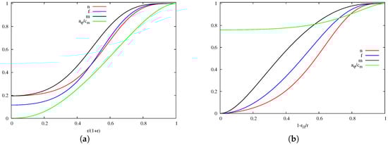
Figure 1. (a) the profiles of a typical soliton with $c_m=2$ and (b) a typical black hole with $r_H=1$ and $c_m=4$. Both profiles correspond to $D=5$ and $L=1$.

4.1. The Solitons

The solitons are fully characterized by the value of the parameter $c_m$, which enters the large$-r$ expansion of the magnetic potential.

The numerical results for $D=5,7,9$ indicate the existence of one single branch of solutions only. This branch starts at $c_m=0$ (which corresponds to vacuum $Ad{S}_D$) and extends continuously up to some limiting value, $c_m=c_m^{*}$. The limiting value $c_m^{*}$ depends on the dimension of the spacetime and L; for $D=5,7,9$, it satisfies with very good accuracy ($0.05\%$) the linear relation

$$c_m^{*}=(1.241+0.2055D)L.$$

(43)

The solutions with $0\le c_m<c_m^{*}$ are regular everywhere. However, the limit $c_m\to c_m^{*}$, is singular, with both the Ricci and the Kretschmann scalars diverging at the origin, $r=0$. In addition, we could not find regular solitons with $c_m>c_m^{*}$. Thus, we conclude that these EM-AdS solitons cannot exist for arbitrarily large values of the magnetic field on the boundary.

In Figure 2a, we show the mass M vs. the parameter $c_m$, the dots marking the position of the limit solutions at $c_m^{*}$. One can notice that the $M\left(c_m\right)$ curve depends on the value of the spacetime dimension. However, the mass remains finite as $c_m\to c_m^{*}$.

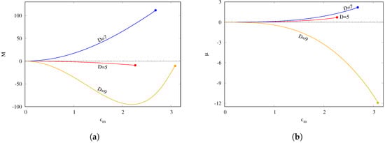
Figure 2. (a) Mass M vs. $c_m$ and (b) μ vs. $c_m$ for static solitons in $D=5$ (red), $D=7$ (blue) and $D=9$ (orange). In both figures, the dots mark the endpoints of the branch of solitons.

In Figure 2b, we show a similar plot for the magnetic moment μ, and again for $D=5$, 7, and 9. One can see that, as expected, the magnitude of the magnetic moment always increases with $c_m$ (note also that the sign of μ is negative in $D=9$).

4.2. The Black Holes

As expected, these solitons possess BH generalizations. In what follows, we will focus on the $D=5$ case, although the described generic properties are expected to hold for any $D=2k+1$.

The magnetized BHs are described by two independent parameters, a natural choice being $c_m$ and the mass M. Then, the solutions can be generated in two ways: (i) by adding a horizon inside the solitons described in the previous Section, or (ii) by introducing a magnetic field into the SAdS BH (which has $c_m=0$).

One important difference with respect to the solitonic case is that, for BHs, the parameter $c_m$ is no longer bounded. However, some basic properties of the solutions now depend on $c_m$ being smaller or larger than the critical value $c_m^{*}$ noticed above for solitons (for $D=5$, one finds $c_m^{*}\simeq 2.269$ for $L=1$).

Let us start by considering families of configurations with fixed values of $c_m$ and varying the temperature. In Figure 3a, we show the mass M vs. the temperature $T_H$ for magnetized BHs with several values of $c_m$. A similar plot is shown in Figure 3b for the horizon area $A_H$ vs. the temperature $T_H$. One can see that, for $0\le c_m<c_m^{*}$, the BHs possess two distinct branches, which we shall call $typeI$ and $typeII$. In the vacuum limit, these correspond to the large and the small branches, respectively, of SAdS BHs. For type I BHs (solid lines), the mass and the horizon area increase with the temperature. For type II BHs (dashed lines), the mass and the horizon area decrease as the temperature increases. This set of BHs is especially interesting, since they can be deformed continuously into solitons, as the horizon size tends to zero.

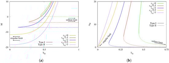
Figure 3. (a) the mass M is shown vs. temperature $T_H$ for static $D=5$ black holes with several different values of the magnetic parameter $c_m$. For $c_m<c_m^{*}$, one finds both type I solutions (continuous lines) and type II solutions (dashed lines). Type II black holes can be deformed into solitons in the limit $T_H\to \infty$. For $c_m>c_m^{*}$, only Type I black holes are present and the limit $T_H\to 0$ is singular; (b) the horizon area $A_H$ is shown vs. temperature $T_H$ for the same solutions. Note that for type II black holes ($c_m<c_m^{*}$), the horizon shrinks to zero as $T_H\to \infty$, a limit which corresponds to a soliton deformation of the AdS background. For $c_m>c_m^{*}$, only Type I solutions are found, while the limit $T_H\to 0$ has $A_H\to 0$, being singular.

Similar to the vacuum SAdS case, these solutions exist above a minimal value of temperature only. This minimal temperature decreases with increasing $c_m$, reaching zero as $c_m=c_m^{*}$. In fact, when $c_m\ge c_m^{*}$, the type II branch completely disappears. Consider for example, the curves for $c_m=2.5$ (orange solid line) and $c_m=3$ (purple solid line) in Figure 3a,b. One can see that only type I BHs are found in these cases, and their temperature can reach $T_H=0$. However, contrary to what happens for the electrically charged Reissner–Nordström-AdS BHs, the extremal limit does not correspond to a regular configuration. Although the mass approaches a finite value there, the horizon area vanishes. In fact, the configurations with $T_H=0$ possess divergent Ricci and Kretschmann scalars at the horizon.

The singular nature of these solutions can also be appreciated in Figure 4a, where we show the deformation parameter ϵ vs. the parameter $c_m$. First, one should notice that $ϵ<1$ for all solutions; thus, a magnetic field increases the relative size of the round $S^{D-3}$ part of the horizon as compared to that of the corresponding $S^1$ part. In addition, one can see that $ϵ\to 0$ as $T_H\to 0$, which likely indicates a change in the topology of the horizon, from spherical to planar.

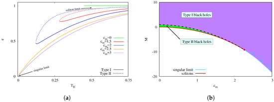
Figure 4. (a) Deformation parameter ϵ vs. $T_H$ for static black holes in $D=5$ for different values of $c_m$ in various colors. Type I solutions are plotted with continuous lines and type II with dashed lines. Note that, in type II BHs ($c_m<c_m^{*}$), the horizon becomes spherical as it shrinks when $T_H\to \infty$, forming a soliton. For $c_m>c_m^{*}$, only Type I is present, and in the limit $T_H\to 0$ the solution becomes singular; (b) mass vs. $c_m$ for static solitons and black holes in $D=5$. In red, we plot the solitons, and the red dot marks the endpoint. The blue line marks the singular limit of black holes. The black dashed line separates the two types of static BHs: Type I (purple area) and Type II (green area). Type II black holes can be contracted to form a soliton.

Finally, in Figure 4b, we show the full domain of existence of the $D=5$ magnetized BHs, in a mass M vs. $c_m$ diagram. This domain is bounded by three different sets of solutions. First, at $c_m=0$, one finds the standard SAdS BHs, with $0\le M<\infty$. For $0\le c_m<c_m^{*}$, the lower bound of the domain of existence is formed by the set of solitons, represented by a red line in Figure 4b. The red dot marks the endpoint of the soliton branch (note that the solitons always possess a lower mass than the BHs with the same $c_m$). However, the BHs exist also for $c_m\ge c_m^{*}$, in which case the lower bound of the domain of existence is no longer given by solitons. Instead, one finds that if one decreases the mass of the BHs, one reaches the singular limit described in the previous paragraphs. This set of singular solutions is plotted as a blue line in Figure 4b.

Then, the magnetized BHs are found in the shaded area, which represent regular configurations with different temperatures. The type I BHs fill the purple area and are always above the configurations with minimum temperatures (that set is marked in Figure 4b with a dashed black line). The type II BHs connect with the soliton limit and fill the green area between the solitons (red line) and the minimum temperature configurations (dashed black line).

5. Conclusions

Some recent results in the literature [16,17,18,19] indicate that, for $D=4$, the known solutions of the EM system in a globally ${\mathrm{AdS}}_4$ background represent only ‘the tip of the iceberg’. New solutions without Minkowski spacetime counterparts were shown to exist (this includes EM solitons), being supported by the confining box behaviour of the AdS spacetime.

The main purpose of this work was to inquire about the possible existence of similar configurations in more than four dimensions. The solutions reported here are likely to be the simplest one can consider in this context. For an odd number of spacetime dimensions, we use a suitable static metric ansatz and a purely $magnetic$ U(1) field, which factorized the angular dependence. As such, the problem reduced to solving a set of ODEs, which significantly simplifies the setup as compared to the $D=4$ case.

Our numerical results in this paper cover the cases $D=5$, 7, and $D=9$, although similar solutions should exist for an arbitrary dimension $D=2k+1$. Some basic results are similar to those known for $D=4$. For example, the existence of solutions can be traced back to the fact that, in contrast to the flat space, the Maxwell equations in an AdS background possess solutions that are finite everywhere. Moreover, these solutions possess self-gravitating generalizations, while a BH can be added at their center.

However, some new features occur as well. For example, for $D>4$, the mass of the solutions, as defined in the usual way, diverges, despite the spacetime being asymptotically AdS, and one has to supplement the boundary action with a matter counterterm. Moreover, for gravitating solitons, one notices the existence of a maximal value of the magnitude of the magnetic potential at infinity for $D>4$.

As avenues for future research, we mention first the issue of electrically charged generalizations, which can be constructed by supplementing the gauge field ansatz with an electric potential,

$$B=a_{\phi }\left(r\right)\left(d\psi +\mathcal{A}\right)+a_0\left(r\right)dt.$$

(44)

One should remark that, although the problem remains codimension-1, the presence of an electric field implies that the solutions necessarily rotate.

Purely electric, static and non-spherically symmetric solutions should exist as well, supported by nontrivial asymptotics of the electric potential. However, they would be less symmetric, with no cohomogeneity-1 ansatz as in this work, and would be found as solutions of partial differential equations. In fact, we have preliminary evidence for the existence of such configurations in $D=5$ dimensions. They share some basic properties of their magnetic counterparts discussed here (for example, their mass as defined in the usual way, diverges logarithmically at infinity).

On a more conceptual level, it would be interesting to consider the solutions in this work in an AdS/CFT context. The fact that, for $D>4$, the EM system (subject to the symmetries in this work) does not correspond to a consistent truncation of a gauged supergravity model makes it more difficult to obtain a CFT description. At the same time, Equation (14) is the basic part of a gauged supergravity action. Thus, we expect some basic properties of the solutions in this work to also hold for generalizations within a supergravity framework. If, for example, one supplements the $D=5$ action with a $U\left(1\right)$ Chern–Simons term, these static black holes are no longer solutions of the theory, unless one considers a planar horizon together with a special gauge field ansatz [39] (see also [40,41]). However, it will certainly be important to study in the future possible extensions of these solutions to Einstein–Maxwell–Chern–Simons theory.

References

- Coleman, S.R. There are no classical glueballs. Commun. Math. Phys. 1977, 55, 113–116. [Google Scholar] [CrossRef]
- Deser, S. Absence of static Einstein-Yang-Mills excitations in three-dimensions. Class. Quant. Grav. 1984, 1, L1. [Google Scholar] [CrossRef]
- Shiromizu, T.; Ohashi, S.; Suzuki, R. A no-go on strictly stationary spacetimes in four/higher dimensions. Phys. Rev. D 2012, 86, 064041. [Google Scholar] [CrossRef]
- Boutaleb-Joutei, H.; Chakrabarti, A.; Comtet, A. Gauge field configurations in curved space-times. Phys. Rev. D 1979, 20, 1884. [Google Scholar] [CrossRef]
- Van der Bij, J.J.; Radu, E. Gravitating sphalerons and sphaleron black holes in asymptotically anti-de Sitter space-time. Phys. Rev. D 2001, 64, 064020. [Google Scholar] [CrossRef]
- Hooft, G. Magnetic monopoles in unified gauge theories. Nucl. Phys. B 1974, 79, 276–284. [Google Scholar] [CrossRef]
- Polyakov, A.M. Particle spectrum in the quantum field theory. JETP Lett. 1974, 20, 430–433. [Google Scholar]
- Hosotani, Y. Scaling behavior in the Einstein-Yang-Mills monopoles and dyons. J. Math. Phys. 2002, 43, 597. [Google Scholar] [CrossRef]
- Bjoraker, J.; Hosotani, Y. Monopoles, dyons and black holes in the four-dimensional Einstein-Yang-Mills theory. Phys. Rev. D 2000, 62, 043513. [Google Scholar] [CrossRef]
- Winstanley, E. Existence of stable hairy black holes in SU(2) Einstein-Yang-Mills theory with a negative cosmological constant. Class. Quant. Grav. 1999, 16, 1963. [Google Scholar] [CrossRef]
- Volkov, M.S.; Gal’tsov, D.V. Non-Abelian Einstein-Yang-Mills black holes. JETP Lett. 1989, 50, 346–350. [Google Scholar]
- Kuenzle, H.P.; Masood-ul-Alam, A.K.M. Spherically symmetric static SU(2) Einstein Yang–Mills fields. J. Math. Phys. 1990, 31, 928. [Google Scholar] [CrossRef]
- Bizon, P. Colored black holes. Phys. Rev. Lett. 1990, 64, 2844. [Google Scholar] [CrossRef] [PubMed]
- Volkov, M.S.; Gal’tsov, D.V. Gravitating non-Abelian solitons and black holes with Yang-Mills fields. Phys. Rep. 1999, 319, 1–83. [Google Scholar] [CrossRef]
- Winstanley, E. Classical Yang-Mills black hole hair in anti-de Sitter space. Lect. Notes Phys. 2009, 769, 49–87. [Google Scholar]
- Herdeiro, C.; Radu, E. Anti-de-Sitter regular electric multipoles: Towards Einstein–Maxwell-AdS solitons. Phys. Lett. B 2015, 749, 393. [Google Scholar] [CrossRef]
- Costa, M.S.; Greenspan, L.; Oliveira, M.; Penedones, J.; Santos, J.E. Polarised Black Holes in AdS. Class. Quant. Grav. 2016, 33, 115011. [Google Scholar] [CrossRef]
- Herdeiro, C.; Radu, E. Einstein–Maxwell-Anti-de-Sitter spinning solitons. Phys. Lett. B 2016, 757, 268. [Google Scholar] [CrossRef]
- Herdeiro, C.A.R.; Radu, E. Static black holes with no spatial isometries in AdS-electrovacuum. Phys. Rev. Lett. 2016, 117, 221102. [Google Scholar] [CrossRef]
- Okuyama, N.; Maeda, K.I. Five-dimensional black hole and particle solution with non-Abelian gauge field. Phys. Rev. D 2003, 67, 104012. [Google Scholar] [CrossRef]
- Radu, E.; Tchrakian, D.H. No hair conjecture, nonAbelian hierarchies and Anti-de Sitter spacetime. Phys. Rev. D 2006, 73, 024006. [Google Scholar] [CrossRef]
- Stotyn, S.; Leonard, C.D.; Oltean, M.; Henderson, L.J.; Mann, R.B. Numerical Boson Stars with a Single Killing Vector I: The D ≥ 5 Case. Phys. Rev. D 2014, 89, 044017. [Google Scholar] [CrossRef]
- Kunz, J.; Navarro-Lérida, F.; Viebahn, J. Charged rotating black holes in odd dimensions. Phys. Lett. B 2006, 639, 362–367. [Google Scholar] [CrossRef]
- Kunz, J.; Navarro-Lérida, F.; Radu, E. Higher dimensional rotating black holes in Einstein–Maxwell theory with negative cosmological constant. Phys. Lett. B 2007, 649, 463–471. [Google Scholar] [CrossRef]
- Clement, G. Classical solutions in three-dimensional Einstein–Maxwell cosmological gravity. Class. Quant. Grav. 1993, 10, L49. [Google Scholar] [CrossRef]
- Hirschmann, E.W.; Welch, D.L. Magnetic solutions to 2+1 gravity. Phys. Rev. D 1996, 53, 5579–5582. [Google Scholar] [CrossRef]
- Cataldo, M.; Salgado, P. Static Einstein–Maxwell solutions in (2+1)-dimensions. Phys. Rev. D 1996, 54, 2971. [Google Scholar] [CrossRef]
- Dias, O.J.C.; Lemos, J.P.S. Rotating magnetic solution in three dimensional Einstein gravity. J. High Energy Phys. 2002. [Google Scholar] [CrossRef]
- Cataldo, M.; Crisostomo, J.; del Campo, S.; Salgado, P. On magnetic solution to 2+1 Einstein–Maxwell gravity. Phys. Lett. B 2004, 584, 123–126. [Google Scholar] [CrossRef]
- Balasubramanian, V.; Kraus, P. A stress tensor for anti-de Sitter gravity. Commun. Math. Phys. 1999, 208, 413–428. [Google Scholar] [CrossRef]
- Das, S.; Mann, R.B. Conserved quantities in Kerr-anti-de Sitter spacetimes in various dimensions. arXiv, 2000; arXiv:hep-th/0008028. [Google Scholar]
- Emparan, R.; Johnson, C.V.; Myers, R.C. Surface terms as counterterms in the AdS/CFT correspondence. Phys. Rev. D 1999, 60, 104001. [Google Scholar] [CrossRef]
- Skenderis, K. Asymptotically Anti-de Sitter space-times and their stress energy tensor. Int. J. Mod. Phys. A 2001, 16, 740–749. [Google Scholar] [CrossRef]
- Taylor, M. More on counterterms in the gravitational action and anomalies. arXiv, arXiv:hep-th/0002125.
- Blázquez-Salcedo, J.L.; Kunz, J.; Navarro-Lérida, F.; Radu, E. Radially excited rotating black holes in Einstein–Maxwell–Chern–Simons theory. Phys. Rev. D 2015, 92, 044025. [Google Scholar] [CrossRef]
- Blázquez-Salcedo, J.L.; Kunz, J.; Navarro-Lérida, F.; Radu, E. Charged rotating black holes in Einstein–Maxwell–Chern–Simons theory with negative cosmological constant. arXiv, 2016; arXiv:1610.05282. [Google Scholar]
- Ascher, U.; Christiansen, J.; Russell, R.D. A collocation solver for mixed order systems of boundary value problems. Math. Comput. 1979, 33, 659–679. [Google Scholar] [CrossRef]
- Ascher, U.; Christiansen, J.; Russell, R.D. Collocation software for boundary-value ODEs. ACM Trans. 1981, 7, 209–222. [Google Scholar] [CrossRef]
- D’Hoker, E.; Kraus, P. Magnetic Brane Solutions in AdS. arXiv, 2009; arXiv:0908.3875. [Google Scholar]
- D’Hoker, E.; Kraus, P. Charged Magnetic Brane Solutions in AdS5 and the fate of the third law of thermodynamics. arXiv, 2010; arXiv:0911.4518. [Google Scholar]
- Ammon, M.; Leiber, J.; Macedo, R.P. Phase diagram of 4D field theories with chiral anomaly from holography. J. High Energy Phys. 2016, 1603, 164. [Google Scholar] [CrossRef]
© 2016 by the authors; licensee MDPI, Basel, Switzerland. This article is an open access article distributed under the terms and conditions of the Creative Commons Attribution (CC-BY) license (http://creativecommons.org/licenses/by/4.0/).