A Bayesian Predictive Discriminant Analysis with Screened Data

Abstract

In the application of discriminant analysis, a situation sometimes arises where individual measurements are screened by a multidimensional screening scheme. For this situation, a discriminant analysis with screened populations is considered from a Bayesian viewpoint, and an optimal predictive rule for the analysis is proposed. In order to establish a flexible method to incorporate the prior information of the screening mechanism, we propose a hierarchical screened scale mixture of normal (HSSMN) model, which makes provision for flexible modeling of the screened observations. An Markov chain Monte Carlo (MCMC) method using the Gibbs sampler and the Metropolis–Hastings algorithm within the Gibbs sampler is used to perform a Bayesian inference on the HSSMN models and to approximate the optimal predictive rule. A simulation study is given to demonstrate the performance of the proposed predictive discrimination procedure.

1. Introduction

The topic of analyzing multivariate screened data has received a great deal of attention over the last few decades. In the standard multivariate problem, an analysis of data generated from a p-dimensional screened random vector $x\stackrel{d}{=}[v|v_0\in {\mathbf{C}}_q)]$ is our issue of interest, where the $p\times 1$ random vector v and the $q\times 1$ random vector $v_0$ (called the screening vector) are jointly distributed with the correlation matrix $Corr(v,v_0^{\top })\ne \mathbf{0}.$ Thus, we observe x only when the unobservable screening vector $v_0$ belongs to a known subset ${\mathbf{C}}_q$ of its space ${\mathbb{R}}^q$, such that $0\le P(v_0\in {\mathbf{C}}_q)\le 1.$ That is, x is subject to the screening scheme or hidden truncation (or simply truncation if $v=v_0$). Model parameters underlying the joint distribution of v and $v_0$ are then estimated from the screened data (i.e., observations of x) using the conditional density $f\left(x\right|v_0\in {\mathbf{C}}_q).$

The screening of sample (or sample selection) arises as open in practice as a result of controlling observability of the outcome of interest in the study. For example, the dataset consists of the Otis IQ test scores (the values of x) of freshmen of a college. These students had been screened in the college admission process, which examines whether their prior school grade point average (GPA) and the Scholastic Aptitude Test (SAT) scores (i.e., the screening values denoted by $v_0$) are satisfactory. What the true vale of screening vector variable $v_0$ of each student is may not be available due to a college regulation. The observations available are the IQ values of x, the screened data. For the application with real screened data, one can refer to that with the student aid grants data given by [1] and that with the U.S. labor market data given by [2], as well. A variety of methods have been suggested for analyzing such screened data. See, e.g., [3,4,5,6], for various distributions for modeling and analyzing screened data; see, [7,8] for the estimative classification analysis with screened data; and see, e.g., [1,2,9,10], for the regression analysis with screened response data.

The majority of existing methods rely on the fact that v and $v_0$ are jointly multivariate normal, and the screened observation vector x is subject to a univariate screening scheme defined by an open interval ${\mathbf{C}}_q$ with $q=1.$ In many practical situations, however, the screened data are generated from a non-normal joint distribution of v and $v_0$, having a multivariate screening scheme defined by a q-dimensional ($q>1$) rectangle region ${\mathbf{C}}_q$ of $v_0.$ In this case, a difficulty in applications with the screened data is that the empirical distribution of the screened data is skewed; its parametric model involves a complex density; and hence, standard methods of analysis cannot be used. See [4,6] for the conditional densities, $f\left(x\right|v_0\in {\mathbf{C}}_q)$, useful for fitting the rectangle screened data generated from a non-normal joint distribution of v and $v_0.$ In this article, we develop yet another multivariate technique applicable for analyzing the rectangle screened data: we are interested in constructing a Bayesian predictive discrimination procedure for the data. More precisely, we consider a Bayesian multivariate technique for sorting, grouping and prediction of multivariate data generated from K rectangle screened populations. In the standard problem, a training sample $\mathcal{D}=\{(z_i,x_i),i=1,\dots ,n\}$ is available, where, for each $i=1,\dots ,n$, $x_i$ is a $p\times 1$ rectangle screened observation vector coming from one of K populations and taking values in ${\mathbb{R}}^p$, and $z_i$ is a categorical response variable representing the population membership, so that $z_i=k$ implies that the predictor $x_i$ belongs to the k-th rectangle screened population (denoted by ${\pi }_k$), $k=1,\dots ,K.$ Using the training sample $\mathcal{D}$, the goal of the predictive discriminant analysis is to predict population membership of a new screened observation x based on the posterior probability of x belonging to ${\pi }_k.$ The posterior probability is given by:

$$\begin{array}{c}\hfill p(z=k|\mathcal{D},x)\propto p(x|\mathcal{D},z=k)p(z=k|\mathcal{D}),k=1,\dots ,K,\end{array}$$

(1)

where z is the the population membership of x, $p(z=k|\mathcal{D})$ is the prior probability of ${\pi }_k$ updated by the training sample $\mathcal{D}$ and:

$$\begin{array}{c}\hfill p\left(x\right|\mathcal{D},z=k)=\int p\left(x\right|{\Theta }_k)p\left({\Theta }_k\right|\mathcal{D},z=k)d{\Theta }_k,\end{array}$$

(2)

$p\left(x\right|{\Theta }_k)=p\left(x\right|v_0\in {\mathbf{C}}_q,z=k)$ and $p\left({\Theta }_k\right|\mathcal{D},z=k)$, respectively, denote the predictive density, the probability density of x and the posterior density of parameters ${\Theta }_k$ associated with ${\pi }_k.$ One of the first and most applied predictive approaches by [11] is the case of unscreened and normally-distributed populations ${\pi }_k$ with unknown parameters ${\Theta }_k=\{{\mathrm{\mu }}_k,{\Sigma }_k\}$, namely ${\pi }_k:N_p({\mu }_k,{\Sigma }_k)$ for $k=1,\dots ,K.$ This is called a Bayesian predictive discriminant analysis with normal populations ($BPD{A}_N$) in which a multivariate Student t distribution is obtained for Equation (2).

A practical example where the predictive discriminant analysis with the rectangle screened populations (${\pi }_k$’s) is applicable is in the discrimination between passed and failed pairs of applicants in a college admission process (the second screening process). Consider the case where college admission officers wish to set up an objective criterion (with a predictor vector x) for admitting students for matriculation; however, the admission officers must first ensure that a student with observation x has passed the first screening process. The first screening scheme may be defined by the q-dimensional region ${\mathbf{C}}_q$ of the random vector $v_0$ (consisting of SAT scores, high-school GPA, and so on), so that only the students who satisfy $v_0\in {\mathbf{C}}_q$ can proceed to the admission process. In this case, we encounter a crucial problem for applying the normal classification by [11]; given the screening scheme $v_0\in {\mathbf{C}}_q$, the assumption of the multivariate normal population distribution for $\left[x\right|z=k]\stackrel{d}{=}\left[x\right|{\pi }_k]$, $k=1,2,\dots ,K$ is not valid. The work in [7,12] found that the normal classification shows a lack of robustness to the departure from the normality of the population distribution, and hence, the performance of the normal classification can be very misleading, if used with the continuous, but non-normal or screened normal input vector x.

Thus, the predictive density in Equation (2) has two specific features to be considered for Bayesian predictive discrimination with the rectangle screened populations, one about the prior distribution of the parameters ${\Theta }_k$ and the other about the distributional assumption of the population model with density $p\left(x\right|{\Theta }_k).$ For the unscreened populations case, there have been a variety of studies that are concerned with the two considerations. See, for example, [11,13,14] for the choice of the prior distributions of ${\Theta }_k$, and see [15,16] for copious references to the literature on the predictive discriminant analysis with non-normal population models. Meanwhile, for deriving Equation (2) of the rectangle screened observation x, we need to develop a population model with density $p\left(x\right|{\Theta }_k)$ that uses the screened sample information in order to maintain consistency with the underlying theory associated with the populations ${\pi }_k$ generating the screened sample. Then, we propose a Bayesian hierarchical approach to flexibly incorporate the prior knowledge about ${\Theta }_k$ with the non-normal sample information, which is the main contribution of this paper to the literature on Bayesian predictive discriminant analysis.

The rest of this paper is organized as follows. Section 2 considers a class of screened scale mixture of normal (SSMN) population models, which well accounts for the screening scheme conducted through a q-dimensional rectangle region ${\mathbf{C}}_q$ of an external scale mixture of normal vector, $v_0.$ Section 3 proposes a hierarchical screened scale mixture of normal (HSSMN) model to derive the predictive density Equation (2) and proposes an optimal rule for Bayesian predictive discriminant analysis (BPDA) with the SSMN populations (abbreviated as $BPD{A}_{SSMN}$). Approximation of the rule is studied in Section 4 by using an MCMC method applied to the HSSMN model. In Section 5, a simulation study is done to check the convergence of the MCMC method and the performance of the $BPD{A}_{SSMN}$ by making a comparison between the $BPD{A}_{SSMN}$ and the $BPD{A}_N.$ Finally, concluding remarks are given in Section 6.

2. The SSMN Population Distributions

Assume that the joint distribution of respective $q\times 1$ and $p\times 1$ vector variables $v_0$ and v, associated with ${\pi }_k$, is $F\in \mathcal{F}$, where:

$$\begin{array}{c}\hfill \mathcal{F}=\left\{F:N_s\left({\mathrm{\mu }}_k^{*},\kappa \left(\mathrm{\eta }\right){\Sigma }_k^{*}\right),\mathrm{\eta }\sim g\left(\mathrm{\eta }\right)\mathrm{with}\kappa \left(\mathrm{\eta }\right)>0,\mathrm{and}\mathrm{\eta }>0\right\},\end{array}$$

(3)

$k=1,\dots ,K$, $s=(q+p)$, η is a mixing variable with the pdf $g\left(\mathrm{\eta }\right)$, $\kappa \left(\mathrm{\eta }\right)$ is a suitably-chosen weight function and ${\mathrm{\mu }}_k^{*}$ and ${\Sigma }_k^{*}$ are partitioned corresponding to the orders of $v_0$ and v:

$$\begin{array}{c}\hfill v^{*}=\left(\begin{array}{c}{v}_0\\ v\end{array}\right),{\mathrm{\mu }}_k^{*}=\left(\begin{array}{c}{\mathrm{\mu }}_{0k}\\ {\mathrm{\mu }}_k\end{array}\right),{\Sigma }_k^{*}=\left(\begin{array}{cc}{\Sigma }_{0k}& {\Delta }_k^{\top }\\ {\Delta }_k& {\Sigma }_k\end{array}\right).\end{array}$$

(4)

Notice that $\mathcal{F}$ defined by Equation (3) denotes a class of scale mixture of multivariate normal (SMN) distributions (see, e.g., [17,18] for details), equivalently denoted as $SM{N}_s({\mathrm{\mu }}_k^{*},{\Sigma }_k^{*},\kappa \left(\mathrm{\eta }\right),G)$ in the remainder of the paper, where $G=G\left(\mathrm{\eta }\right)$ denote the cdf of $\mathrm{\eta }.$

Given the joint distribution $\left[v^{*}\right|{\pi }_k]\sim SM{N}_s({\mathrm{\mu }}_k^{*},{\Sigma }_k^{*},\kappa \left(\mathrm{\eta }\right),G)$, the SSMN distribution is defined by the following screening scheme:

$$\left[x\right|{\pi }_k]\stackrel{d}{=}\left[v\right|v_0\in {\mathbf{C}}_q(\alpha ,\beta ),{\pi }_k]\sim SSM{N}_p({\mathbf{C}}_q(\alpha ,\beta );{\mathrm{\mu }}_k^{*},{\Sigma }_k^{*},\kappa \left(\mathrm{\eta }\right),G),$$

(5)

where ${\mathbf{C}}_q(\alpha ,\beta )=\{v_0\in {\mathbb{R}}^q|\alpha \le v_0\le \beta \}$ is a q-dimensional rectangle screening region in the space of $v_0\in {\mathbb{R}}^q.$ Here, $\alpha ={({\alpha }_1,\cdots ,{\alpha }_q)}^T$, $\beta ={({\beta }_1,\cdots ,{\beta }_q)}^T$, and ${\alpha }_j<{\beta }_j$ for $j=1,\cdots ,q$. This region contains the cases of ${\mathbf{C}}_q(\alpha ,\infty )$ and ${\mathbf{C}}_q(-\infty ,\beta )$ as special cases.

The pdf of x is given by:

$$f\left(x\right|{\mathrm{\mu }}_k^{*},{\Sigma }_k^{*},{\pi }_k)=\frac{{\int }_0^{\infty }{h}_p\left(x\right|{\mathrm{\mu }}_k^{*},{\Sigma }_k^{*},\kappa \left(\mathrm{\eta }\right),G)dG\left(\mathrm{\eta }\right)}{{\int }_0^{\infty }{\overline{\Phi }}_q({\mathbf{C}}_q(\alpha ,\beta );{\mathrm{\mu }}_{0k},\kappa \left(\mathrm{\eta }\right){\Sigma }_{0k})dG\left(\mathrm{\eta }\right)},x\in {\mathbb{R}}^p,$$

(6)

where:

$$h_p\left(x\right|{\mathrm{\mu }}_k^{*},{\Sigma }_k^{*},\kappa \left(\mathrm{\eta }\right))={\varphi }_p(x;{\mathrm{\mu }}_k,\kappa \left(\mathrm{\eta }\right){\Sigma }_k){\overline{\Phi }}_q\left({\mathbf{C}}_q(\alpha ,\beta );{\mathrm{\mu }}_{v_{0k}|x},\kappa \left(\mathrm{\eta }\right){\Sigma }_{v_{0k}|x}\right),$$

${\mathrm{\mu }}_{v_{0k}|x}={\mathrm{\mu }}_{0k}+{\Delta }_k^{\top }{\Sigma }_k^{-1}(x-{\mathrm{\mu }}_k)$ and ${\Sigma }_{v_{0k}|x}={\Sigma }_{0k}-{\Delta }_k^{\top }{\Sigma }_k^{-1}{\Delta }_k.$ Here, ${\varphi }_q(·\mathrm{\mu },\Sigma )$ and ${\overline{\Phi }}_q({\mathbf{C}}_q(\alpha ,\beta );\mathrm{\mu },\Sigma )$, respectively, denote the pdf and the probability of the rectangle region of a random vector $w\sim N_q(\mathrm{\mu },\Sigma )$. The latter is equivalent to $Pr(w\in {\mathbf{C}}_q(\alpha ,\beta )).$

One particular member of the class of SSMN distributions is the rectangle-screened normal (RSN) distribution defined by Equation (5) and Equation (6), for which $G\left(\mathrm{\eta }\right)$ is degenerate with $\kappa \left(\mathrm{\eta }\right)=1$. The work in [4,8] studied properties of the distribution and denoted it as the $RS{N}_p({\mathbf{C}}_q(\alpha ,\beta );{\mathrm{\mu }}_k^{*},{\Sigma }_k^{*})$ distribution. Another member of the class is the rectangle-screened p-variate Student t distributions ($RS{t}_p$) considered by [8]. Its pdf is given by:

$$f\left(x\right|{\mathrm{\mu }}_k^{*},{\Sigma }_k^{*},{\pi }_k)=t_p\left(x\right|{\mathrm{\mu }}_k,{\Sigma }_k,\mathrm{\nu })\frac{{\overline{T}}_q\left({\mathbf{C}}_q(\alpha ,\beta );{\mathrm{\mu }}_{v_{0k}|x},{\Gamma }_{v_{0k}|x},\mathrm{\nu }+p\right)}{{\overline{T}}_q({\mathbf{C}}_q(\alpha ,\beta );{\mathrm{\mu }}_{0k},{\Sigma }_{0k},\mathrm{\nu })},x\in {\mathbb{R}}^p,$$

(7)

where $t_p(·|\mathbf{a},B,c)$ and ${\overline{T}}_p({\mathbf{C}}_p;\mathbf{a},B,c)$ are the respective pdf and probability of a rectangle region ${\mathbf{C}}_p$ of the p-variate Student t distribution with the location vector $\mathbf{a}$, the scale matrix B, the degrees of freedom c and:

$${\Gamma }_{v_{0k}|x}={(\mathrm{\nu }+p)}^{-1}\left\{\mathrm{\nu }+{(x-{\mathrm{\mu }}_k)}^{\top }{\Sigma }_k^{-1}(x-{\mathrm{\mu }}_k)\right\}{\Sigma }_{v_{0k}|x}.$$

Similar to the RSN distributions, the density Equation (7) of $\left[x\right|{\pi }_k]\sim RS{t}_p({\mathbf{C}}_q(\alpha ,\beta );{\mathrm{\mu }}_k^{*},{\Sigma }_k^{*},\mathrm{\nu })$ is obtained by taking $\kappa \left(\mathrm{\eta }\right)=1/\mathrm{\eta }$ and $\mathrm{\eta }\sim Gamma(\mathrm{\nu }/2,\mathrm{\nu }/2)$, i.e.,

$$g\left(\mathrm{\eta }\right)=\frac{{(\mathrm{\nu }/2)}^{\mathrm{\nu }/2}}{\Gamma (\mathrm{\nu }/2)}{\mathrm{\eta }}^{\mathrm{\nu }/2-1}exp\left\{-\frac{\mathrm{\nu }}{2}\mathrm{\eta }\right\},\mathrm{\eta }>0.$$

The stochastic representations of the RSN and $RS{t}_p$ distributions are immediately obtained by applying the following lemma, for which detailed proof can be found in [4].

Lemma 1. Suppose $\left[x\right|{\pi }_k]\sim SSM{N}_p({\mathbf{C}}_q(\alpha ,\beta );{\mathrm{\mu }}_k^{*},{\Sigma }_k^{*},\kappa \left(\mathrm{\eta }\right),G)$. Then, it has the following stochastic representation in a hierarchical fashion,

$$\begin{array}{ccc}\hfill \left[x\right|\mathrm{\eta },{\pi }_k]& \stackrel{d}{=}& {\mathrm{\mu }}_k+{\Delta }_k{\Sigma }_{0k}^{-1}{\mathbf{Z}}_{{\mathbf{C}}_q(a_k,b_k)}+{({\Sigma }_k-{\Delta }_k{\Sigma }_{0k}^{-1}{\Delta }_k^{\top })}^{1/2}{\mathbf{Z}}_p,\hfill \end{array}$$

(8)

$$\begin{array}{ccc}\hfill \mathrm{\eta }& \sim & G\left(\mathrm{\eta }\right)with\kappa \left(\mathrm{\eta }\right)>0,\mathrm{\eta }>0,\hfill \end{array}$$

(9)

where ${\mathbf{Z}}_p\sim N_p(\mathbf{0},\kappa \left(\mathrm{\eta }\right)I_p)$ and ${\mathbf{Z}}_{{\mathbf{C}}_q-{\mathrm{\mu }}_{0k}}\stackrel{d}{=}\left[{\mathbf{Z}}_q\right|{\mathbf{Z}}_q\in {\mathbf{C}}_q(a_k,b_k)]$ are conditionally independent and ${\mathbf{Z}}_q\sim N_q(\mathbf{0},\kappa \left(\mathrm{\eta }\right){\Sigma }_{0k})$. Here, $a_k=\alpha -{\mathrm{\mu }}_{0k}$ and $b_k=\beta -{\mathrm{\mu }}_{0k}.$

Lemma 1 provides the following: (i) an intrinsic structure of the SSMN population distributions, which reveals a type of departure from the SMN law because the distribution of $\left[x\right|{\pi }_k]$ reduces to the SMN distribution if ${\Delta }_k=\mathbf{0}$ (i.e., $Cov(v_0,v|{\pi }_k)=\mathbf{0}$); (ii) the representation provides a convenient device for random number generation; (iii) it leads to a simple and direct construction of a HSSMN model for the BPDA with the SSMN populations, i.e., $\left[x\right|{\pi }_k]\sim SSM{N}_p({\mathbf{C}}_q(\alpha ,\beta );{\mathrm{\mu }}_k^{*},{\Sigma }_k^{*},\kappa \left(\mathrm{\eta }\right),G)$.

3. The HSSMN Model

3.1. The Hierarchical Model

For a Bayesian predictive discriminant analysis, suppose we have K rectangle screened populations ${\pi }_k(k=1,\dots ,K)$, each specified by the $SSM{N}_p({\mathbf{C}}_q(\alpha ,\beta );{\mathrm{\mu }}_k^{*},{\Sigma }_k^{*},\kappa \left(\mathrm{\eta }\right),G)$ distribution. Let ${\mathcal{D}}_k=\{x_{k1},\dots ,x_{k{n}_k}\}$ be a training sample obtained from the rectangle screened population ${\pi }_k$ with the $SSM{N}_p({\mathbf{C}}_q(\alpha ,\beta );{\mathrm{\mu }}_k^{*},{\Sigma }_k^{*},\kappa \left(\mathrm{\eta }\right),G)$ distribution, where the parameters (${\mathrm{\mu }}_k^{*},{\Sigma }_k^{*})$ are unknown. The predictive discrimination analysis is to assess the relative predictive odds ratio or posterior probability that a screened multivariate observation x belongs to one of K populations, ${\pi }_k.$ As noted by Equation (6), however, a complex likelihood function of ${\mathcal{D}}_k$ prevents us from choosing reasonable priors of the model parameters and obtaining the predictive density of x given by Equation (2). These problems are solved if we use the following hierarchical representation of the population models.

According to Lemma 1, we may rewrite the SSMN model for Equations (8) and (9) by a three-level hierarchy given by:

$$\begin{array}{ccc}\hfill \left[x_{ki}\right|{\mathrm{\eta }}_{ki},f_{ki},{\pi }_k]& \stackrel{d}{=}& {\mathrm{\mu }}_k+{\Lambda }_k{f}_{ki}+{\epsilon }_{ki},{\epsilon }_{ki}\stackrel{ind}{\sim }{N}_p(\mathbf{0},\kappa \left({\mathrm{\eta }}_{ki}\right){\Psi }_k),i=1,\dots ,n_k,\hfill \end{array}$$

(10)

$$\begin{array}{ccc}\hfill f_{ki}& \stackrel{ind}{\sim }& N_q(\mathbf{0},\kappa \left({\mathrm{\eta }}_{ki}\right){\Sigma }_{0k})I\left(f_{ki}\in {\mathbf{C}}_q(a_k,b_k)\right),\kappa \left({\mathrm{\eta }}_{ki}\right)>0,\hfill \end{array}$$

$$\begin{array}{ccc}\hfill {\mathrm{\eta }}_{ki}& \stackrel{i.i.d.}{\sim }& G\left(\mathrm{\eta }\right)with{\mathrm{\eta }}_{ki}>0,\hfill \end{array}$$

where ${\Lambda }_k={\Delta }_k{\Sigma }_{0k}^{-1}$, ${\Psi }_k={\Sigma }_k-{\Delta }_k{\Sigma }_{0k}^{-1}{\Delta }_k^{\top }$, G is the scale mixing distribution of the independent ${\mathrm{\eta }}_{ki}$’s, $f_{ki}$ and ${\epsilon }_{ki}$ are independent conditional on ${\mathrm{\eta }}_{ki}$ and $N_q(\mathbf{0},\kappa \left({\mathrm{\eta }}_{ki}\right){\Sigma }_{0k})I\left(f_{ki}\in {\mathbf{C}}_q(a_k,b_k)\right)$ denotes a truncated $N_q(\mathbf{0},\kappa \left({\mathrm{\eta }}_{ki}\right){\Sigma }_{0k})$ distribution having the truncated space $f_{ki}\in {\mathbf{C}}_q(a_k,b_k).$

The first stage model in Equation (10) may be written in a compact form by defining the following vector and matrix notations,

$$\begin{array}{cc}& {\mathbf{X}}_k=(x_{k1}-{\mathrm{\mu }}_k,\dots ,x_{k{n}_k}-{\mathrm{\mu }}_k),{\mathbf{F}}_k=(f_{k1},\dots ,f_{k{n}_k}),\\ & {\mathbf{E}}_k=({\epsilon }_{k1},\dots ,{\epsilon }_{k{n}_k}),{\mathrm{\eta }}_k={({\mathrm{\eta }}_{k1},\dots ,{\mathrm{\eta }}_{k{n}_k})}^{\top }.\end{array}$$

Then, the three-level hierarchy of the model Equation (10) can be expressed as:

$$\begin{array}{ccc}\hfill {\mathbf{X}}_k& =& {\Lambda }_k{\mathbf{F}}_k+{\mathbf{E}}_k,vec\left({\mathbf{E}}_k\right)\sim N_{p{n}_k}(\mathbf{0},D(\kappa \left({\mathrm{\eta }}_k\right))\otimes \Psi ),\hfill \end{array}$$

(11)

$$\begin{array}{ccc}\hfill vec\left({\mathbf{F}}_k\right)& \sim & N_{q{n}_k}(\mathbf{0},D(\kappa \left({\mathrm{\eta }}_k\right))\otimes {\Sigma }_{0k})I(f_{ki}\in {\mathbf{C}}_q\left(a_k,b_k)\right),\mathrm{Cov}(vec\left({\mathbf{F}}_k\right),vec{\left({\mathbf{E}}_k\right)}^{\top }|{\mathrm{\eta }}_k)=\mathbf{O},\hfill \end{array}$$

$$\begin{array}{ccc}\hfill {\mathrm{\eta }}_{ki}& \stackrel{i.i.d.}{\sim }& g\left(\mathrm{\eta }\right),i=1,\dots ,n_k,\hfill \end{array}$$

where $\mathbf{A}\otimes \mathbf{B}$ denotes the Kronecker product of two matrices $\mathbf{A}$ and $\mathbf{B}$, $vec\left({\mathbf{F}}_k\right)={(f_{k1}^{\top },\dots ,f_{k{n}_k}^{\top })}^{\top }$, $vec\left({\mathbf{E}}_k\right)={({\epsilon }_{k1}^{\top },\dots ,{\epsilon }_{k{n}_k}^{\top })}^{\top }$, and $D(\kappa \left({\mathrm{\eta }}_k\right))=diag\{\kappa \left({\mathrm{\eta }}_{k1}\right),\dots ,\kappa \left({\mathrm{\eta }}_{k{n}_k}\right)\}$ is an $n_k\times n_k$ diagonal matrix of the scale mixing functions. Note that the hierarchical population model Equation (11) adopts a robust discriminant modeling by the use of the scale mixture of normal, such as the SMN and the truncated SMN, and thus, it enables us to avoid the anomaly generated from the non-normal sample information.

The Bayesian analysis of the model in Equation (11) begins with the specification of the prior distributions of the unknown parameters. When the prior information is not available, a convenient strategy of avoiding improper posterior distribution is to use proper priors with their hyperparameters being fixed as appropriate quantities to reflect the flatness (or diffuseness) of priors (i.e., limiting non-informative priors). For convenience, but not always optimal, we suppose that ${\mathrm{\mu }}_k$, ${\mathrm{\mu }}_{0k}$, $({\Lambda }_k,{\Psi }_k)$ and ${\Sigma }_{0k}$ of the model in Equation (11) are independent a priori; prior distributions for ${\mathrm{\mu }}_k$ and ${\mathrm{\mu }}_{0k}$ are normal; an inverse Wishart prior distribution for ${\Sigma }_{0k}$; and a generalized natural conjugate family (see [19]) of prior distributions for $({\Lambda }_k,{\Psi }_k)$, so that we adopt the normal prior density for the ${\Lambda }_k$ conditional on the matrix ${\Psi }_k$,

$$\begin{array}{ccc}\hfill P\left({\Lambda }_k\right|{\Psi }_k)& \sim & |{\Psi }_k{|}^{-q/2}exp\left\{-\frac{1}{2}tr[{\Psi }_k^{-1}({\Lambda }_k-{\Lambda }_{0k})H_k{({\Lambda }_k-{\Lambda }_{0k})}^{\top }]\right\},\hfill \\ \hfill {\Psi }_k& \sim & I{W}_p(R_k,{\tau }_k),\hfill \end{array}$$

where $W\sim I{W}_m(V,\mathrm{\nu })$ denotes the inverse Wishart distribution whose pdf $I{W}_m(W;V,\mathrm{\nu })$ is:

$$I{W}_m(W;V,\mathrm{\nu })\propto {\left|W\right|}^{-\mathrm{\nu }/2}exp\left\{-\frac{1}{2}tr\left(W^{-1}V\right)\right\},V>0.$$

Note that if ${\Lambda }_k=({\lambda }_{k1},\dots ,{\lambda }_{kq})$, ${\lambda }_k\equiv vec\left({\Lambda }_k\right)={({\lambda }_{k1}^{\top },\dots ,{\lambda }_{kq}^{\top })}^{\top }$ and ${\lambda }_{0k}\equiv vec\left({\Lambda }_{0k}\right)$, then:

$$tr[{\Psi }_k^{-1}({\Lambda }_k-{\Lambda }_{0k})H_k{({\Lambda }_k-{\Lambda }_{0k})}^{\top }]={({\lambda }_k-{\lambda }_{0k})}^{\top }{(H_k^{-1}\otimes {\Psi }_k)}^{-1}({\lambda }_k-{\lambda }_{0k}).$$

This prior elicitation of the parameters, along with the three-level hierarchical model Equation (11), produces a hierarchical screened scale mixture of normal population model, which is referred to as HSSMN($\Theta \left(k\right)$) in the rest of this paper, where $\Theta \left(k\right)=\{{\mathrm{\mu }}_k,{\mathrm{\mu }}_{0k},{\Lambda }_k,{\Psi }_k,{\mathbf{F}}_k,{\Sigma }_{0k},{\mathrm{\eta }}_k\}.$ The HSSMN($\Theta \left(k\right)$) model is defined as follows.

$$\begin{array}{ccc}\hfill \left[x_{ki}|{\mathbf{F}}_k,{\mathrm{\mu }}_k,{\Psi }_k,{\mathrm{\eta }}_k\right]& \stackrel{ind}{\sim }& N_p({\mathrm{\mu }}_k+{\Lambda }_k{f}_{ki},\kappa \left({\mathrm{\eta }}_{ki}\right){\Psi }_k),i=1,\dots ,n_k,\hfill \end{array}$$

(12)

$$\begin{array}{ccc}\hfill \left[f_{ki}|{\Psi }_k,{\Sigma }_{0k},{\mathrm{\mu }}_{0k},{\mathrm{\eta }}_k\right]& \stackrel{ind}{\sim }& N_q\left(\mathbf{0},\kappa \left({\mathrm{\eta }}_{ki}\right){\Sigma }_{0k}\right)I\left(f_{ki}\in {\mathbf{C}}_q(a_k,b_k)\right),i=1,\dots ,n_k,\hfill \end{array}$$

$$\begin{array}{ccc}\hfill {\mathrm{\mu }}_k& \sim & N_p({\theta }_k,{\Omega }_k),\hfill \end{array}$$

$$\begin{array}{ccc}\hfill {\mathrm{\mu }}_{0k}& \sim & N_q({\theta }_{0k},{\Omega }_{0k}),\hfill \end{array}$$

$$\begin{array}{ccc}\hfill \left[{\lambda }_k|{\Psi }_k\right]& \sim & N_{pq}({\lambda }_{0k},H_k^{-1}\otimes {\Psi }_k),\hfill \end{array}$$

$$\begin{array}{ccc}\hfill {\Psi }_k& \sim & I{W}_p(R_k,{\tau }_k),{\tau }_k>2p,\hfill \end{array}$$

$$\begin{array}{ccc}\hfill {\Sigma }_{0k}& \sim & I{W}_q(Q_k,{\gamma }_k),{\gamma }_k>2q,\hfill \end{array}$$

$$\begin{array}{ccc}\hfill {\mathrm{\eta }}_{ki}& \stackrel{ind}{\sim }& g\left(\mathrm{\eta }\right),i=1,\dots ,n_k,\hfill \end{array}$$

where ${\lambda }_k\equiv vec\left({\Lambda }_k\right)$, ${\lambda }_{0k}\equiv vec\left({\Lambda }_{0k}\right)$ and hyperparameters $({\theta }_k,{\theta }_{0k},{\Omega }_k,{\Omega }_{0k},{\Lambda }_{0k},H_k,R_k,{\tau }_k,Q_k,{\gamma }_k)$ are fixed as appropriate quantities to reflect the flatness of priors.

The last distributional specification is omitted in the RSN distribution case. For the HSSMN($\Theta \left(k\right)$) model for the $RS{t}_{\mathrm{\nu }}$ distribution, we may set ${\mathrm{\eta }}_{ki}\stackrel{ind}{\sim }Gamma(\mathrm{\nu }/2,\mathrm{\nu }/2)$, $\mathrm{\nu }\sim Gamma(1,0.1)I(\mathrm{\nu }>2)$, a truncated Gamma distribution (see, e.g., [20]). See, for example, [21,22] and the references therein for other choices of the prior distribution of $\mathrm{\nu }.$

3.2. Posterior Distributions

Based on the HSSMN($\Theta \left(k\right)$) model structure with the likelihood and the prior distributions in Equation (12), the joint posterior distribution of $\Theta \left(k\right)$ is given by:

$$\begin{array}{ccc}\hfill p(\Theta \left(k\right)|{\mathcal{D}}_k)& \propto & \left(\prod _{i=1}^{n_k}{|\kappa \left({\mathrm{\eta }}_{ki}\right){\Psi }_k|}^{-1/2}\right)exp\left\{-\frac{1}{2}tr\left[{\Psi }_k^{-1}({\mathbf{X}}_k-{\Lambda }_k{\mathbf{F}}_k)\mathbf{D}{(\kappa \left({\mathrm{\eta }}_k\right))}^{-1}{({\mathbf{X}}_k-{\Lambda }_k{\mathbf{F}}_k)}^{\top }\right]\right\}\hfill \end{array}$$

$$\begin{array}{ccc}& \times & |{\Psi }_k{|}^{-(q+{\tau }_k)/2}exp\left\{-\frac{1}{2}tr\left[{\Psi }_k^{-1}{G}_k\right]\right\}\prod _{i=1}^{n_k}\frac{{\varphi }_q(f_{ki};\mathbf{0},\kappa \left({\mathrm{\eta }}_{ki}\right){\Sigma }_{0k})}{{\overline{\Phi }}_q\left({\mathbf{C}}_q(a_k,b_k);\mathbf{0},\kappa \left({\mathrm{\eta }}_{ki}\right){\Sigma }_{0k}\right)}\left(\prod _{i=1}^{n_k}g\left({\mathrm{\eta }}_{ki}\right)\right)\hfill \end{array}$$

$$\begin{array}{ccc}& \times & I{W}_q({\Sigma }_{0k};Q_k,{\gamma }_k){\varphi }_p({\mathrm{\mu }}_k;{\theta }_k,{\Omega }_k){\varphi }_q({\mathrm{\mu }}_{0k};{\theta }_{0k},{\Omega }_{0k}),\hfill \end{array}$$

(13)

where:

$$\begin{array}{ccc}& & \left(\prod _{i=1}^{n_k}{|\kappa \left({\mathrm{\eta }}_{ki}\right){\Psi }_k|}^{-1/2}\right)exp\left\{-\frac{1}{2}tr\left[{\Psi }_k^{-1}({\mathbf{X}}_k-{\Lambda }_k{\mathbf{F}}_k)\mathbf{D}{(\kappa \left({\mathrm{\eta }}_k\right))}^{-1}{({\mathbf{X}}_k-{\Lambda }_k{\mathbf{F}}_k)}^{\top }\right]\right\}\hfill \\ & \propto & \prod _{i=1}^{n_k}{\varphi }_p(x_{ki};{\mathrm{\mu }}_k+{\Lambda }_k{f}_{ki},\kappa \left({\mathrm{\eta }}_{ki}\right){\Psi }_k),\hfill \end{array}$$

$G_k=({\Lambda }_k-{\Lambda }_{0k})H_k{({\Lambda }_k-{\Lambda }_{0k})}^{\top }+R_k$ and $g\left({\mathrm{\eta }}_{ki}\right)$’s denote the densities of the mixing variables ${\mathrm{\eta }}_{ki}$’s. Note that the joint posterior of Equation (13) is not simplified in an analytic form of the known density and, thus, intractable for the posterior inference. Instead, we derived each of conditional posterior distribution of ${\mathrm{\mu }}_k$, ${\mathrm{\mu }}_{0k}$, ${\lambda }_k\equiv vec\left({\Lambda }_k\right)$, ${\Sigma }_{0k}$, ${\mathbf{F}}_k$, ${\Psi }_k$ and ${\mathrm{\eta }}_{ki}$’s, which will be useful for posterior inference based on Markov chain Monte Carlo methods (MCMC). All of the full conditional posterior distributions are as follows (see the Appendix for their derivations):

(1) The full conditional distribution of ${\mathrm{\mu }}_k$ is a p-variate normal given by:

$$\left[{\mathrm{\mu }}_k{|\Theta \left(k\right)}_{\backslash {\mathrm{\mu }}_k},{\mathcal{D}}_k\right]\sim N_p\left({\mathrm{\mu }}_{{\mathrm{\mu }}_k},{\Sigma }_{{\mathrm{\mu }}_k}\right),$$

(14)

where ${\mathrm{\mu }}_{{\mathrm{\mu }}_k}={\Sigma }_{{\mathrm{\mu }}_k}\left({\Omega }_k^{-1}{\theta }_k+{\sum }_{i=1}^{n_k}{\Psi }_k^{-1}(x_{ki}-{\Lambda }_k{f}_{ki})/\kappa \left({\mathrm{\eta }}_{ki}\right)\right)$ and ${\Sigma }_{{\mathrm{\mu }}_k}={\left({\sum }_{i=1}^{n_k}\frac{1}{\kappa \left({\mathrm{\eta }}_{ki}\right)}{\Psi }_k^{-1}+{\Omega }_k^{-1}\right)}^{-1}.$

(2) The full conditional density of ${\mathrm{\mu }}_{0k}$ is given by:

$$\begin{array}{c}\hfill p({\mathrm{\mu }}_{0k}|\Theta {\left(k\right)}_{\backslash {\mathrm{\mu }}_{0k}},{\mathcal{D}}_k)\propto \frac{{\varphi }_q({\mathrm{\mu }}_{0k};{\theta }_{0k},{\Omega }_{0k})}{{\prod }_{i=1}^{n_k}{\overline{\Phi }}_q\left({\mathbf{C}}_q(\alpha ,\beta );{\mathrm{\mu }}_{0k},\kappa \left({\mathrm{\eta }}_{ki}\right){\Sigma }_{0k}\right)}.\end{array}$$

(15)

(3) The full conditional posterior distribution of ${\lambda }_k$ is given by:

$$\left[{\lambda }_k{|\Theta \left(k\right)}_{\backslash {\lambda }_k},{\mathcal{D}}_k\right]\sim N_{pq}\left({\mathrm{\mu }}_{{\lambda }_k},{\Sigma }_{{\lambda }_k}\right),$$

(16)

where:

$$\begin{array}{ccc}\hfill {\mathrm{\mu }}_{{\lambda }_k}& =& vec\left({\Lambda }_k^{*}\right),{\Lambda }_k^{*}=({\mathbf{X}}_k\mathbf{D}{(\kappa \left({\mathrm{\eta }}_k\right))}^{-1}{\mathbf{F}}_k^{\top }+{\Lambda }_{0k}{H}_k)Q_k^{-1}\hfill \\ \hfill {\Sigma }_{{\lambda }_k}& =& Q_k^{-1}\otimes {\Psi }_k,and{Q}_k={\mathbf{F}}_k\mathbf{D}{(\kappa \left({\mathrm{\eta }}_k\right))}^{-1}{\mathbf{F}}_k^{\top }+H_k.\hfill \end{array}$$

(4) The full conditional posterior distribution of ${\Psi }_k$ is an inverse-Wishart distribution:

$$\left[{\Psi }_k{|\Theta \left(k\right)}_{\backslash {\Psi }_k},{\mathcal{D}}_k\right]\sim I{W}_p\left(V_k,{\mathrm{\nu }}_k\right){\mathrm{\nu }}_k>2p,$$

(17)

where $V_k=({\mathbf{X}}_k-{\Lambda }_k{\mathbf{F}}_k)\mathbf{D}{(\kappa \left({\mathrm{\eta }}_k\right))}^{-1}{({\mathbf{X}}_k-{\Lambda }_k{\mathbf{F}}_k)}^{\top }+({\Lambda }_k-{\Lambda }_{0k})H_k{({\Lambda }_k-{\Lambda }_{0k})}^{\top }+R_k$ and ${\mathrm{\nu }}_k=n_k+q+{\tau }_k.$

(5) The full conditional posterior distribution of $f_{ki}$ is the q-variate truncated normal given by:

$$\left[f_{ki}{|\Theta \left(k\right)}_{\backslash f_{ki}},{\mathcal{D}}_k\right]\stackrel{ind}{\sim }{N}_q\left({\mathrm{\mu }}_{f_{ki}},\kappa \left({\mathrm{\eta }}_{ki}\right){\Sigma }_{f_{ki}}\right)I\left(f_{ki}\in {\mathbf{C}}_q(a_k,b_k)\right),i=1,\dots ,n_k,$$

(18)

where ${\mathrm{\mu }}_{f_{ki}}={\Sigma }_{f_{ki}}{\Lambda }_k^{\top }{\Psi }_k^{-1}(x_{ki}-{\mathrm{\mu }}_k)$ and ${\Sigma }_{f_{ki}}={\left({\Sigma }_{0k}^{-1}+{\Lambda }_k^{\top }{\Psi }_k^{-1}{\Lambda }_k\right)}^{-1}.$

(6) The full conditional posterior density of ${\Sigma }_{0k}$ is given by:

$$p({\Sigma }_{0k}|\Theta {\left(k\right)}_{\backslash {\Sigma }_{0k}},{\mathbf{y}}_k)\propto I{W}_q({\Sigma }_{0k};Q_k,{\gamma }_k)\prod _{i=1}^{n_k}\frac{{\varphi }_q(f_{ki};\mathbf{0},\kappa \left({\mathrm{\eta }}_{ki}\right){\Sigma }_{0k})}{{\overline{\Phi }}_q\left({\mathbf{C}}_q(a_k,b_k);\mathbf{0},\kappa \left({\mathrm{\eta }}_{ki}\right){\Sigma }_{0k}\right)}.$$

(19)

(7) The full conditional posterior densities of ${\mathrm{\eta }}_{ki}$’s are given by:

$$\begin{array}{ccc}\hfill p({\mathrm{\eta }}_{ki}|\Theta {\left(k\right)}_{\backslash {\mathrm{\eta }}_{ki}},{\mathbf{y}}_k)& \propto & \kappa {\left({\mathrm{\eta }}_{ki}\right)}^{-\frac{p}{2}}exp\left\{-\frac{z_{ki}^{\top }{\Psi }_k^{-1}{z}_{ki}}{2\kappa \left({\mathrm{\eta }}_{ki}\right)}\right\}\hfill \end{array}$$

(20)

$$\begin{array}{ccc}& \times & \frac{{\varphi }_q(f_{ki};\mathbf{0},\kappa \left({\mathrm{\eta }}_{ki}\right){\Sigma }_{0k})}{{\overline{\Phi }}_q\left({\mathbf{C}}_q(a_k,b_k);\mathbf{0},\kappa \left({\mathrm{\eta }}_{ki}\right){\Sigma }_{0k}\right)}g\left({\mathrm{\eta }}_{ki}\right),i=1,\dots ,n_k,\hfill \end{array}$$

where $z_{ki}=x_{ki}-{\mathrm{\mu }}_k-{\Lambda }_k{f}_{ki}$ and ${\mathrm{\eta }}_{ki}$’s are independent.

Based on the above full conditional posterior distributions and the stochastic representations of the SSMN in Lemma 1, one can easily obtain Bayes estimates of the k-th SSMN population mean ${\mathrm{\mu }}_{{\pi }_k}=E\left[x\right|{\pi }_k]$ and covariance matrix ${\Sigma }_{{\pi }_k}=Cov\left(x\right|{\pi }_k)$, $k=1,\dots ,K.$ Specifically, the mean and covariance matrix of an observation x belonging to ${\pi }_k:SSM{N}_p({\mathbf{C}}_q(\alpha ,\beta );{\mathrm{\mu }}_k^{*},{\Sigma }_k^{*},\kappa \left(\mathrm{\eta }\right),G)$, which are used for calculating their Bayes estimates via Rao–Blackwellization, are given by:

$$\begin{array}{ccc}\hfill {\mathrm{\mu }}_{{\pi }_k}& =& {\mathrm{\mu }}_k+{\Omega }_{21k}{\Omega }_{22k}^{-1}{\xi }_k\hfill \end{array}$$

(21)

$$\begin{array}{ccc}\hfill {\Sigma }_{{\pi }_k}& =& {\Omega }_{22k}-{\Omega }_{21k}({\Omega }_{11k}^{-1}-{\Omega }_{11k}^{-1}{\mathbf{T}}_k{\Omega }_{11k}^{-1}){\Omega }_{21k}^{\top },\hfill \end{array}$$

where ${\Omega }_{21k}=\kappa \left(\mathrm{\eta }\right){\Delta }_k$, ${\Omega }_{11k}=\kappa \left(\mathrm{\eta }\right){\Sigma }_{0k}$, ${\Omega }_{22k}=\kappa \left(\mathrm{\eta }\right){\Sigma }_k$,

$${\xi }_k={\int }_{{\mathbf{C}}_q(a_k,b_k)}\frac{\mathbf{z}}{{\zeta }_k{(2\pi )}^{q/2}{\left|{\Omega }_{11k}\right|}^{1/2}}exp\{-\frac{{\mathbf{z}}^{\top }{\Omega }_{11k}^{-1}\mathbf{z}}{2}\}d\mathbf{z},$$

${\zeta }_k={\overline{\Phi }}_q({\mathbf{C}}_q(\alpha ,\beta );{\mathrm{\mu }}_{0k},{\Omega }_{11k})$, ${\mathbf{T}}_k={\mathbf{P}}_k-{\xi }_k{\xi }_k^{\top }$ and:

$${\mathbf{P}}_k={\int }_{{\mathbf{C}}_q(a_k,b_k)}\frac{\mathbf{z}{\mathbf{z}}^{\top }}{{\zeta }_k{(2\pi )}^{q/2}{\left|{\Omega }_{11k}\right|}^{1/2}}exp\{-\frac{{\mathbf{z}}^{\top }{\Omega }_{11k}^{-1}\mathbf{z}}{2}\}d\mathbf{z}.$$

We see that these moments of Equation (21) agree with the formula for the mean and covariance matrix of the untruncated marginal distribution of a general multivariate truncated distribution given by [23]. Readers are referred to [24] with the R package tmvtnorm and [25] with the R package mvtnorm for implementing calculations of ${\xi }_k$ and ${\mathbf{P}}_k$ involved in the first and second moments.

When the sampling information, i.e., the observed training samples, is augmented by the proper information of prior knowledge, the anomalies of the maximum likelihood estimate of the SSMN model, investigated by [16], would disappear in the HSSMN $(\Theta (k\left)\right)$ model. Furthermore, note that the conditional distribution of ${\lambda }_k$ in Equation (16) is a $pq$-dimensional one; and hence, its Gibbs sampling needs to be performed by using the inverse of the matrix of order $pq$, which may cause computational costs in implementing the MCMC method. For large q, a more computationally-convenient Gibbs sampler can be considered based on the full conditional posterior distributions of ${\lambda }_{kj}$, $j=1,\dots ,p$, than the Gibbs sampler with ${\lambda }_k$ in Equation (16), where ${\lambda }_k\equiv Vec\left({\Lambda }_k\right)$ and ${\Lambda }_k\equiv ({\lambda }_{k1},\dots ,{\lambda }_{kq}).$

For this purpose, we defined the following notations: for $j=1,\dots ,p$,

$${\tilde{\lambda }}_k\left(j\right)=(E_j\otimes I_p){\lambda }_k,{\tilde{\theta }}_k\left(j\right)=(E_j\otimes I_p){\mathrm{\mu }}_{{\lambda }_k},$$

$${\tilde{\Omega }}_k\left(j\right)=(E_j\otimes I_p){\Sigma }_{{\lambda }_k}{(E_j\otimes I_p)}^{\top },E_i={({\mathbf{e}}_j,{\mathbf{e}}_1,\dots ,{\mathbf{e}}_{j-1},{\mathbf{e}}_{j+1},\dots ,{\mathbf{e}}_q)}^{\top },$$

where ${\mathbf{e}}_j$ denotes the j-th column of $I_q$, namely an elementary vector with unity for its j-th element and zeros elsewhere. Furthermore, we consider the following partitions:

$${\tilde{\lambda }}_k\left(j\right)=\left(\begin{array}{c}{\lambda }_{kj}\\ {\lambda }_{kj}^{*}\end{array}\right),{\tilde{\theta }}_k\left(j\right)=\left(\begin{array}{c}{\tilde{\theta }}_k\left(1j\right)\\ {\tilde{\theta }}_k\left(2j\right)\end{array}\right),and{\tilde{\Omega }}_k\left(j\right)=\left(\begin{array}{cc}{\tilde{\Omega }}_{k11}\left(j\right)& {\tilde{\Omega }}_{k12}\left(j\right)\\ {\tilde{\Omega }}_{k21}\left(j\right)& {\tilde{\Omega }}_{k22}\left(j\right)\end{array}\right),$$

where the orders of ${\lambda }_{kj}^{*}$, ${\tilde{\theta }}_k\left(1j\right)$, ${\tilde{\Omega }}_{k11}\left(j\right)$ and ${\tilde{\Omega }}_{k21}\left(j\right)$ are $(p-1)q\times 1$, $q\times 1$, $q\times q$ and $(p-1)q\times q$, respectively. Under these partitions, the conditional property of a multivariate normal distribution leads to the full conditional posterior distributions of ${\lambda }_{kj}$ given by:

$$\begin{array}{c}\hfill \left[{\lambda }_{kj}{|\Theta \left(k\right)}_{\backslash {\lambda }_{kj}},{\mathbf{y}}_k\right]\sim N_q\left({\mathrm{\mu }}_{{\lambda }_{kj}},{\Sigma }_{{\lambda }_{kj}}\right),\end{array}$$

(22)

for $j=1,\dots ,q$, where:

$${\mathrm{\mu }}_{{\lambda }_{kj}}={\tilde{\theta }}_k\left(1j\right)+{\tilde{\Omega }}_{k12}{\tilde{\Omega }}_{k22}^{-1}({\lambda }_{kj}^{*}-{\tilde{\theta }}_k\left(2j\right))and{\Sigma }_{{\lambda }_{kj}}={\tilde{\Omega }}_{k11}\left(j\right)-{\tilde{\Omega }}_{k12}\left(j\right){\tilde{\Omega }}_{k22}{\left(j\right)}^{-1}{\tilde{\Omega }}_{k21}\left(j\right).$$

When p is large, we may partition ${\lambda }_{kj}$ into two vectors with smaller dimensions, say ${\lambda }_k={({\lambda }_{kj}{\left(1\right)}^{\top },{\lambda }_{kj}\left(2\right){,}^{\top })}^{\top }$, then use their full conditional normal distributions for the Gibbs sampler.

Now, the posterior sampling can be implemented by using all of the conditional posterior Equations (14)–(20). The Gibbs sampler and Metropolis–Hastings algorithm within the Gibbs sampler may be used to obtain posterior samples of all of the unknown parameters $\Theta \left(k\right)$. Note that in the case where the $pq$-dimensional matrix is too large to manipulate for computation, the Gibbs sampler can be modified by replacing the full conditional posterior Equation (16) with Equation (22). That is, as indicated by Equation (22), the modified Gibbs sampler based on Equation (22) would be more convenient for numerical computation than the first one using Equation (16). The detailed Markov chain Monte Carlo algorithm with Gibbs sampling is discussed in the next subsection.

3.3. Markov Chain Monte Carlo Sampling Scheme

It is not complicated to construct an MCMC sampling scheme working with $\Theta \left(k\right)=\{{\mathrm{\mu }}_k,{\mathrm{\mu }}_{0k},{\Lambda }_k,{\Psi }_k,{\mathbf{F}}_k,{\Sigma }_{0k},{\mathrm{\eta }}_k\}$, since a routine Gibbs sampler would work to generate posterior samples of $({\mathrm{\mu }}_k,{\Lambda }_k,{\Psi }_k,{\mathbf{F}}_k)$ based on each of their full conditional posterior distributions obtained in Section 3.2. In the posterior sampling of ${\mathrm{\mu }}_{0k}$, ${\Sigma }_{0k}$ and ${\mathrm{\eta }}_k$, Metropolis–Hastings within the Gibbs algorithm would be used, since their conditional posterior densities do not have explicit forms of known distributions as in Equation (15), Equation (19) and Equation (20).

Here, for simplicity, we considered the MCMC algorithm based on the HSSMN$(\Theta (k\left)\right)$ model with a known screening scheme, in which ${\mathrm{\mu }}_{0k}$ and ${\Sigma }_{0k}$ are assumed to be known. The extension to the general HSSMN$(\Theta (k\left)\right)$ model with unknown ${\mathrm{\mu }}_{0k}$ and ${\Sigma }_{0k}$ can be made without difficulty.

The MCMC algorithm starts with some initial values ${\mathrm{\mu }}_k^{\left[0\right]}$, ${\lambda }_k^{\left[0\right]}$, ${\Psi }_k^{\left[0\right]}$, ${\mathbf{F}}_k^{\left[0\right]}$ and ${\mathrm{\eta }}_k^{\left[0\right]}.$ The detailed posterior sampling steps are as follows:

• Step 1: generate ${\mathrm{\mu }}_k$ by using the full conditional posterior distribution in Equation (14).
• Step 2: generate ${\lambda }_k$ by using the full conditional posterior distribution in Equation (16).
• Step 3: generate inverse-Wishart random matrix ${\psi }_k$ by using the full conditional posterior distribution in Equation (17).
• Step 4: generate independent q-variate truncated normal random variables $f_{ki}$ by using the full conditional posterior distribution in Equation (18).
• Step 5: given the current values $\{{\mathrm{\mu }}_k,{\Lambda }_k,{\Psi }_k,{\mathbf{F}}_k\}$, we independently generate a candidate ${\mathrm{\eta }}_{ki}$ from a proposal density $q\left({\mathrm{\eta }}_{ki}^{*}\right|{\mathrm{\eta }}_{ki})=g\left({\mathrm{\eta }}_{ki}^{*}\right)$, as suggested by [26], which is used for a Metropolis–Hastings algorithm. Then, accept the candidate value with the acceptance rate:

  $$\alpha ({\mathrm{\eta }}_{ki},{\mathrm{\eta }}_{ki}^{*})=min\left\{\frac{p(\Theta \left(k\right)|{\mathrm{\eta }}_{ki}^{*})}{p(\Theta \left(k\right)|{\mathrm{\eta }}_{ki}\left)\right)},1\right\}$$

  $i=1,\dots ,n_k.$ Because the target density is proportional to $p(\Theta \left(k\right)|{\mathrm{\eta }}_{ki})g\left({\mathrm{\eta }}_{ki}\right)$ and $p(\Theta \left(k\right)|{\mathrm{\eta }}_{ki})$ is uniformly bounded for ${\mathrm{\eta }}_{ik}>0$ where:

  $$\begin{array}{ccc}\hfill p(\Theta \left(k\right)|{\mathrm{\eta }}_{ki})& =& {\varphi }_p(x_{ki};{\mathrm{\mu }}_k+{\Lambda }_k{f}_{ki},\kappa \left({\mathrm{\eta }}_{ki}\right){\Psi }_k)\frac{{\varphi }_q(f_{ki};\mathbf{0},\kappa \left({\mathrm{\eta }}_{ki}\right){\Sigma }_{0k})}{{\overline{\Phi }}_q\left({\mathbf{C}}_q(a_k,b_k);\mathbf{0},\kappa \left({\mathrm{\eta }}_{ki}\right){\Sigma }_{0k}\right)}\hfill \end{array}$$

  and $g(·)$ is the density of mixing variable ${\mathrm{\eta }}_{ik}$. Note that ${\mathrm{\eta }}_k={({\mathrm{\eta }}_{k1},\dots ,{\mathrm{\eta }}_{k{n}_k})}^{\top }.$

When one conducts a posterior inference of the HSSMN ($\Theta \left(k\right)$) model using the samples obtained from the MCMC sampling algorithm, the following points should be noted.

(i)

See, e.g., [18], for the sampling method for ${\mathrm{\eta }}_{ki}$ from various mixing distributions $g\left({\mathrm{\eta }}_{ki}\right)$ of the SMN distributions, such as the multivariate t, multivariate $logit$ , multivariate $stable$ and multivariate $exponential$ $power$ models.

(ii)

Suppose the HSSMN($\Theta \left(k\right)$) model involves unknown ${\mathrm{\mu }}_{0k}.$ Then, as indicated by the full conditional posterior of ${\mathrm{\mu }}_{0k}$ in Equation (15), the complexity of the conditional distribution prevents us from using straightforward Gibbs sampling. Instead, we may use a simple random walk Metropolis algorithm that uses a normal proposal density $q\left({\mathrm{\mu }}_{0k}^{*}\right|{\mathrm{\mu }}_{0k})=q\left(\right|{\mathrm{\mu }}_{0k}^{*}-{\mathrm{\mu }}_{0k}\left|\right)$ to sample from the conditional distribution of ${\mathrm{\mu }}_{0k}^{*}$; that is, given the current point is ${\mathrm{\mu }}_{0k}$, the candidate point is ${\mathrm{\mu }}_{0k}^{*}\sim N_q({\mathrm{\mu }}_{0k},D)$, where a diagonal matrix D should be turned, so that the acceptance rate of the candidate point is around 0.25 (see, e.g., [26]).

(iii)

When the HSSMN($\Theta \left(k\right)$) model involves unknown ${\Sigma }_{0k}$: The MCMC sampling algorithm, using the full conditional posterior Equation (19) is not straightforward, because the conditional posterior density is unknown and complex. Instead, we may apply a Metropolized hit-and-run algorithm, described by [27], to sample from the conditional posterior of ${\Sigma }_{0k}.$

(iv)

One can easily calculate the posterior estimate of ${\Theta }_k=({\mathrm{\mu }}_k^{*},{\Sigma }_k^{*})$ by using that of $\Theta \left(k\right)$, because the re-parameterizing relations are $\Psi ={\Sigma }_k-{\Delta }_k{\Sigma }_{0k}^{-1}{\Delta }_k^{\top }$ and ${\Lambda }_k={\Delta }_k{\Sigma }_{0k}^{-1}.$

4. The Predictive Classification Rule

Suppose we have K populations ${\pi }_k$, $k=1,\dots ,K$, each specified by the HSSMN$(\Theta (k\left)\right)$ model. For each of the populations, we have the screened training sample ${\mathcal{D}}_k$ comprised of a set of independent observations $\{x_{ki},i=1,\dots ,n_k\}$ whose population level is $z_{ki}=k.$ Let x be assigned to one of the K populations, with prior probability $p_k$ of belonging to ${\pi }_k$, ${\sum }_{k=1}^K{p}_k=1.$ Then, the predictive density of x given $\mathcal{D}$ under the HSSMN$(\Theta (k\left)\right)$ model with the space $\Theta \left(k\right)\in \Theta \left(k\right)$ is:

$$\begin{array}{c}\hfill p\left(x\right|\mathcal{D},z=k)={\int }_{\Theta \left(k\right)}^{}p\left(x\right|\Theta \left(k\right))p(\Theta \left(k\right)|\mathcal{D})d\Theta \left(k\right),k=1,\dots ,K,\end{array}$$

(23)

and the posterior probability that x belongs to ${\pi }_k$, i.e., $p(z=k|\mathcal{D},x)=p(x\in {\pi }_k|\mathcal{D},x)$, is:

$$\begin{array}{c}\hfill p(x\in {\pi }_k|\mathcal{D},x)=\frac{p\left(x\right|\mathcal{D},z=k\left)p\right(z=k\left|\mathcal{D}\right)}{{\sum }_{j=1}^{K}p\left(x\right|\mathcal{D},z=j)p(z=j|\mathcal{D})},k=1,\dots ,K,\end{array}$$

(24)

where $\mathcal{D}={\bigcup }_{k=1}^K{\mathcal{D}}_k$, $p\left(x\right|\Theta \left(k\right))$ is equal to Equation (6) and $p(\Theta (k\left)\right|\mathcal{D})$ is the joint posterior density given in Equation (13). We see from Equation (24) that the total posterior probability of misclassifying x from ${\pi }_i$ to ${\pi }_j$, $i\ne j$ is defined by:

$$\begin{array}{c}\hfill TPM\left(j\right)=\sum _{i\ne j;i=1}^K\frac{p\left(x\right|\mathcal{D},z=i\left)p\right(z=i\left|\mathcal{D}\right)}{{\sum }_{\ell =1}^{K}p\left(x\right|\mathcal{D},z=\ell )p(z=\ell |\mathcal{D})}.\end{array}$$

(25)

We minimize the misclassification error at this point if we choose j, so as to minimize Equation (25); that is, we select k that gives the maximum posterior probability $p(x\in {\pi }_k|\mathcal{D},x)$ (see, e.g., Theorem 6.7.1 of [28] (p. 234). Thus, an optimal Bayesian predictive discrimination rule that minimizes the classification error is to classify x into ${\pi }_k$, if $x\in R_k$, where the optimal classification region is given by:

$$\begin{array}{c}\hfill R_k:p\left(x\right|\mathcal{D},z=k)p(z=k|\mathcal{D})>p\left(x\right|\mathcal{D},z=j)p(z=j|\mathcal{D}),\mathrm{for} \mathrm{all}j\ne k;k=1,\dots ,K,\end{array}$$

(26)

$p(z=k|\mathcal{D})$ is the posterior probability of population ${\pi }_k$ given the dataset $\mathcal{D}.$ If we assume the values of $p_k$’s are a priori known, then $p(z=k|\mathcal{D})=p_k.$

Since we are unable to obtain an analytic solution of Equation (26), a numerical approach is required. Thus, we used the MCMC method of the previous section to draw samples from the posterior density of the parameters, $p(\Theta (k\left)\right|\mathcal{D})$, to approximate the predictive density, Equation (23), by:

$$\begin{array}{c}\hfill p\left(x\right|\mathcal{D},z=k)\approx \frac{1}{N_k-M}\sum _{t=M+1}^{N_k}p\left(x\right|{\Theta }_k^t),k=1,\dots ,K,\end{array}$$

(27)

where ${\Theta }_k^t$’s are posterior samples generated from the MCMC process under the HSSMN$(\Theta (k\left)\right)$ model and M and $N_k$ are the burn-in period and run length, respectively.

If we assume Dirichlet priors for $p_k$, that is:

$$[p_1,\dots ,p_{K-1}]\sim Dirichlet(d_1,\dots ,d_{K-1};d_K)$$

(see, e.g., [19] (p. 143) for the distributional properties), then:

$$\begin{array}{c}\hfill p(z=k|\mathcal{D})=E\left[p_k\right|\mathcal{D}]=\frac{d_k+n_k}{{\sum }_j^K{d}_j+n_j},k=1,\dots ,K-1\end{array}$$

(28)

and $p(z=K|\mathcal{D})=1-{\sum }_{j=k}^{K-1}p(z=k|\mathcal{D}).$

Thus, the posterior probabilities in Equation (24) and the minimum error classification region $R_k$ in Equation (26) can be generated within the MCMC scheme, which uses Equation (27) to approximate the predictive densities involved in Equation (24) and Equation (26).

5. Simulation Study

This section presents results of a simulation study to show the convergence of the MCMC algorithm and the performance of the $BPD{A}_{SSMN}$. Simulation of the training sample observations, model estimation by the MCMC algorithm and a comparison of classification results among three BPDA methods were implemented by coding the R package program. The three methods consist of two proposed $BPD{A}_{SSMN}$ methods (i.e., $BPD{A}_{RSN}$ and $BPD{A}_{RSt}$ for classifying RSN and RSt populations) and $BPD{A}_N$ by [11] (for classifying unscreened normal populations).

5.1. A Simulation Study: Convergence of the MCMC Algorithm

This simulation study considers inference of the HSSMN$(\Theta (k\left)\right)$ model with a two-dimensional case by generating a training sample of one thousand observations, $n_k=1000$, from each population ${\pi }_k$, $k=1,2,3.$ We considered the following specific choice of parameters, i.e., ${\mathrm{\mu }}_k={({\mathrm{\mu }}_{k1},{\mathrm{\mu }}_{k2})}^{\top }$, ${\Sigma }_{0k}$, ${\mathrm{\mu }}_{0k}$, ${\mathbf{C}}_q(\alpha ,\beta )$, ${\lambda }_k=Vec\left({\Lambda }_k^{\top }\right)={({\lambda }_{k1},\dots ,{\lambda }_{k4})}^{\top }$ and ${\Psi }_k={\Sigma }_k-{\Delta }_k{\Sigma }_{0k}^{-1}{\Delta }_k=\left\{{\psi }_{kij}\right\}$ matrices, for generating a synthetic data from ${\pi }_k$,

$$\begin{array}{ccc}\hfill {\mathrm{\mu }}_k& =& \left(\begin{array}{c}1+k\\ -2+k\end{array}\right),{\Sigma }_{0k}=\left(\begin{array}{cc}7+{\epsilon }_k& -2\\ -2& 4+{\epsilon }_k\end{array}\right),\alpha =\left(\begin{array}{c}-0.5\\ -0.5\end{array}\right),\beta =\left(\begin{array}{c}4\\ 4\end{array}\right),\hfill \\ \hfill {\mathrm{\mu }}_{0k}& =& {(0,0)}^{\top },{\Delta }_k=\left(\begin{array}{cc}2& 1\\ 2& 0\end{array}\right),{\Sigma }_k=\left(\begin{array}{cc}3+{\epsilon }_k& 0\\ 0& 1+{\epsilon }_k\end{array}\right),and{\epsilon }_k=0.1\times k.\hfill \end{array}$$

Based on the above parameter values with $p=q=2$, we simulated 200 sets of three training samples of each size $n_k=1000$ from three populations ${\pi }_k$, $k=1,2,3.$ Two cases of screened populations were assumed, that is ${\pi }_k:RS{N}_p({\mathbf{C}}_q(\alpha ,\beta );{\mathrm{\mu }}_k^{*},{\Sigma }_k^{*})$ and ${\pi }_k:RS{t}_p({\mathbf{C}}_q(\alpha ,\beta );{\mathrm{\mu }}_k^{*},{\Sigma }_k^{*},\mathrm{\nu }=5).$ The respective datasets were generated by using the stochastic representation of each population (see Lemma 1 for the representation). Given a generated training sample, corresponding population parameters were estimated by using the MCMC algorithm based on the HSSMN$(\Theta (k\left)\right)$ model, Equation (12), for each screened population, ${\pi }_k$, distribution. We used ${\mathrm{\mu }}_k=\mathbf{0}$, ${\Delta }_k=I_2$ and ${\Psi }_k=I_2$ as the initial values of the MCMC algorithm. To satisfy an objective Bayesian perspective considered by [29], we need to specify the hyper-parameters $({\theta }_k,{\delta }_k,{\Omega }_k,{\Omega }_{0k},H_k,R_k,Q_k,{\tau }_k,{\gamma }_k)$ of the HSSMN$(\Theta (k\left)\right)$ model, so as to be insensitive to changes of the priors. Thus, we assumed that we have no information about the parameters. To specify this, we adopted ${\theta }_k=\mathbf{0}$, ${\delta }_k=\mathbf{0}$, ${\Omega }_k={10}^3{I}_p$, ${\Omega }_{0k}={10}^3{I}_q$, $H_k={10}^{-3}{I}_q$, $R_k={10}^{-3}{I}_p$, $Q_k={10}^{-3}{I}_q$, ${\tau }_k={10}^{-3}+p+1$ and ${\gamma }_k={10}^{-3}+q+1$ (see, e.g., [18]).

The MCMC samplers were based on 20,000 iterations as burn-in, followed by a further 20,000 iterations with a thinning size of 10. Thus, the final MCMC samples with a size of 2000 were obtained for each HSSMN$(\Theta (k\left)\right)$ model. Table 1 only provides posterior summaries for the parameters of the ${\pi }_1$ distribution for the sake of saving space. From Column 4–Column 9 of the table list, the mean and three quantiles of 200 sets of posterior samples, which were obtained from the MCMC method, were repeatedly applied to the 200 sets of training sample of size $n_1=1000.$ Then, the remaining two columns of the table list formal convergence test results of the MCMC algorithm. In estimating the Monte Carlo error (MC error) in Column 5, we used the batch mean method with 50 batches, see e.g., [30] (pp. 39–40). The low values of the MC errors indicate that the variability of each estimate due to the simulation is well controlled. The table also compares the MCMC results with the true parameter values (listed in Column 3): (i) each parameter value in Column 3 is located in the credible interval (2.5% quantile, 97.5% quantile); (ii) for each parameter, we see that the difference between its true value and corresponding posterior mean is less than 2 × the standard error (s.e.). Thus, the posterior summaries, obtained by using the weakly informative priors, indicate that the MCMC method based on the HSSMN$(\Theta (1\left)\right)$ model performs well in estimating the population parameters, regardless of the SSMN models (RSN and RSt) considered.

Table 1. Posterior summaries of 200 Markov chain Monte Carlo (MCMC) results for the ${\pi }_1$ models.

Model (${\pi }_1$)	Parameter	True	Mean	MC Error	s.e.	2.5%	Median	97.5%	$R_c$	p-Value
RSN	${\mathrm{\mu }}_{11}$	2.000	1.966	0.003	0.064	1.882	1.964	2.149	1.014	0.492
	${\mathrm{\mu }}_{12}$	−1.000	−0.974	0.002	0.033	−1.023	−0.974	−0.903	1.011	0.164
	${\lambda }_{11}$	0.312	0.320	0.008	0.159	0.046	0.322	0.819	1.021	0.944
	${\lambda }_{12}$	0.406	0.407	0.007	0.164	0.030	0.417	0.872	1.018	0.107
	${\lambda }_{13}$	0.250	0.253	0.004	0.083	0.082	0.256	0.439	1.019	0.629
	${\lambda }_{14}$	0.125	0.133	0.004	0.067	0.003	0.133	0.408	1.017	0.761
	${\psi }_{111}$	1.968	2.032	0.005	0.130	1.743	2.008	2.265	1.034	0.634
	${\psi }_{112}$	−0.625	−0.627	0.002	0.098	−0.821	−0.617	−0.405	1.022	0.778
	${\psi }_{122}$	0.500	0.566	0.001	0.039	0.465	0.557	0.638	1.018	0.445
RSt	${\mathrm{\mu }}_{11}$	2.000	2.036	0.004	0.069	1.867	2.050	2.166	1.015	0.251
	${\mathrm{\mu }}_{12}$	−1.000	−1.042	0.003	0.036	−1.137	−1.054	−0.974	1.012	0.365
	${\lambda }_{11}$	0.312	0.318	0.008	0.072	0.186	0.320	0.601	1.017	0.654
	${\lambda }_{12}$	0.406	0.405	0.006	0.074	0.262	0.414	0.562	1.019	0.712
	${\lambda }_{13}$	0.250	0.255	0.005	0.051	0.113	0.257	0.387	1.023	0.661
	${\lambda }_{14}$	0.125	0.136	0.005	0.055	0.027	0.133	0.301	1.019	0.598
	${\psi }_{111}$	1.968	1.906	0.006	0.108	1.781	1.996	2.211	1.023	0.481
	${\psi }_{112}$	−0.625	−0.620	0.003	0.101	−0.818	−0.615	−0.422	1.021	0.541
	${\psi }_{122}$	0.500	0.459	0.002	0.044	0.366	0.457	0.578	1.016	0.412

Table 1. Posterior summaries of 200 Markov chain Monte Carlo (MCMC) results for the ${\pi }_1$ models.

Model (${\pi }_1$)	Parameter	True	Mean	MC Error	s.e.	2.5%	Median	97.5%	$R_c$	p-Value
RSN	${\mathrm{\mu }}_{11}$	2.000	1.966	0.003	0.064	1.882	1.964	2.149	1.014	0.492
	${\mathrm{\mu }}_{12}$	−1.000	−0.974	0.002	0.033	−1.023	−0.974	−0.903	1.011	0.164
	${\lambda }_{11}$	0.312	0.320	0.008	0.159	0.046	0.322	0.819	1.021	0.944
	${\lambda }_{12}$	0.406	0.407	0.007	0.164	0.030	0.417	0.872	1.018	0.107
	${\lambda }_{13}$	0.250	0.253	0.004	0.083	0.082	0.256	0.439	1.019	0.629
	${\lambda }_{14}$	0.125	0.133	0.004	0.067	0.003	0.133	0.408	1.017	0.761
	${\psi }_{111}$	1.968	2.032	0.005	0.130	1.743	2.008	2.265	1.034	0.634
	${\psi }_{112}$	−0.625	−0.627	0.002	0.098	−0.821	−0.617	−0.405	1.022	0.778
	${\psi }_{122}$	0.500	0.566	0.001	0.039	0.465	0.557	0.638	1.018	0.445
RSt	${\mathrm{\mu }}_{11}$	2.000	2.036	0.004	0.069	1.867	2.050	2.166	1.015	0.251
	${\mathrm{\mu }}_{12}$	−1.000	−1.042	0.003	0.036	−1.137	−1.054	−0.974	1.012	0.365
	${\lambda }_{11}$	0.312	0.318	0.008	0.072	0.186	0.320	0.601	1.017	0.654
	${\lambda }_{12}$	0.406	0.405	0.006	0.074	0.262	0.414	0.562	1.019	0.712
	${\lambda }_{13}$	0.250	0.255	0.005	0.051	0.113	0.257	0.387	1.023	0.661
	${\lambda }_{14}$	0.125	0.136	0.005	0.055	0.027	0.133	0.301	1.019	0.598
	${\psi }_{111}$	1.968	1.906	0.006	0.108	1.781	1.996	2.211	1.023	0.481
	${\psi }_{112}$	−0.625	−0.620	0.003	0.101	−0.818	−0.615	−0.422	1.021	0.541
	${\psi }_{122}$	0.500	0.459	0.002	0.044	0.366	0.457	0.578	1.016	0.412

Some of the trace plots from an MCMC run are provided in Figure 1. Each plot demonstrates a parallel zone centered near the true parameter value of interest with no obvious tendency or periodicity. These plots and the small MC error values listed in Table 1 convince us of the convergence of the MCMC algorithm. For a formal diagnostic check, we calculated the Brooks and Gelman diagnostic statistic $R_c$ (adjusted shrinkage factor introduced by [31]) using a MCMC runs with three chains in parallel, each one starting from different initial values. The calculated $R_c$ value for each parameter is listed in the 10th column of Table 1. Table 1 shows that all of the $R_c$ values are close to one, indicating the convergence of the MCMC algorithm. For another formal diagnostic check, we applied the Heidelberger–Welch diagnostic tests of [32] to single-chain MCMC runs, which were used to plot Figure 1. They consist of the stationarity test and the half-width test for the MCMC runs of each parameter. The 11th column of Table 1 lists the p-value of the test for the stationarity of the single Markov chain, where all of the p-values are larger than 0.1. Furthermore, all of the the half-width tests, testing the convergence of the Markov chain of a single parameter, were passed. Thus, all of the diagnostic checking methods (formal and informal methods) advocate the convergence of the proposed MCMC algorithm, and hence, we can say that it generates an MCMC sample that comes from the marginal posterior distributions of interest (i.e., the SSMN population parameters). It is seen that the similar estimation results in Table 1 apply to the posterior summaries of the other parameters in ${\pi }_2$ and ${\pi }_3$ distributions. According to these simulation results, we can say that the MCMC algorithm constructed in Section 3.3 provides an efficient method for estimating the SSMN distributions. To achieve this quality of MCMC algorithm for the higher dimensional case (with large p and/or q values), the diagnostic tests, considered in this section, should be used to monitor the convergence of the algorithm; for more details, see [30].

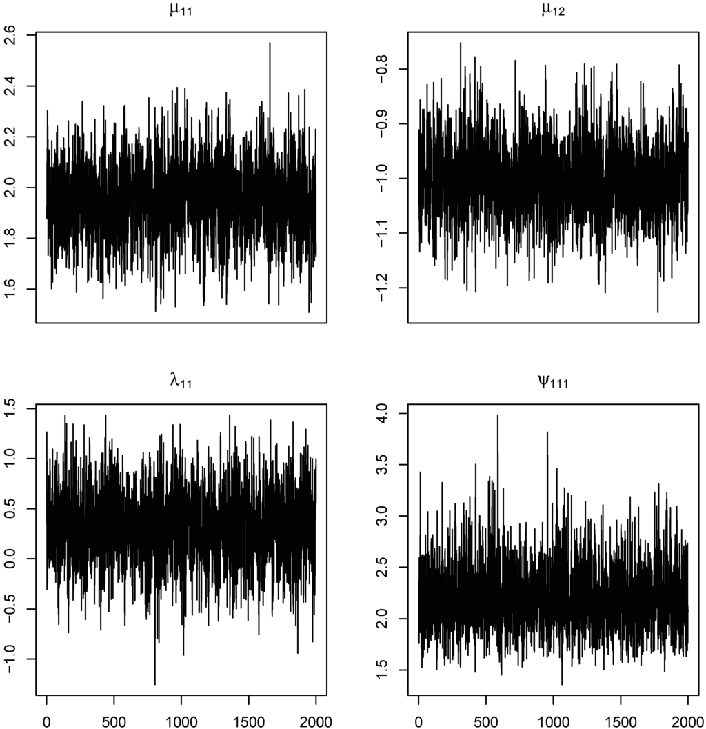
Figure 1. Trace plots of ${\mathrm{\mu }}_{11}$, ${\mathrm{\mu }}_{12}$, ${\lambda }_{11}$ and ${\psi }_{111}$ generated from HSSMN$(\Theta (1\left)\right)$ of the RSt with $\mathrm{\nu }=5$ model.

5.2. A Simulation Study: Performance of the Predictive Methods

This simulation study compares the performance of three BPDA methods using training samples generated from three rectangle screened populations, ${\pi }_k$ ($k=1,2,3$). The three methods compared are $BPD{A}_{RSN}$, $BPD{A}_{RSt}$ with degrees of freedom $\mathrm{\nu }=5$, and $BPD{A}_N$ (a standard predictive method with no screening). Two different cases of rectangle screened population distributions were used to generate the training samples. One case is the rectangle screened population ${\pi }_k$ with the $RS{N}_p({\mathbf{C}}_q(\alpha ,\beta );{\mathrm{\mu }}_k^{*},{\Sigma }_k^{*})$ distribution. The other case is ${\pi }_k$ with the $RS{t}_p({\mathbf{C}}_q(\alpha ,\beta );{\mathrm{\mu }}_k^{*},{\Sigma }_k^{*},\mathrm{\nu }=5)$ distribution in order to examine the robustness of $BPD{A}_{RSt}$ in discriminating observations from heavily-tailed empirical distributions. For each case, we obtained 200 sets of training and validation (or testing) samples of each size $n_k=20,50,100$ generated from the rectangle screened distribution of ${\pi }_k.$ They are denoted by ${\mathcal{D}}_k\left(i\right)$ and ${\mathcal{V}}_k\left(i\right)(i=1,\dots ,200).$ The i-th validation sample ${\mathcal{V}}_k\left(i\right)$ that corresponds to the training ${\mathcal{D}}_k\left(i\right)$ sample was simply obtained by setting ${\mathcal{V}}_k\left(i\right)={\mathcal{D}}_k(i-1)(i=1,\dots ,200)$, where ${\mathcal{D}}_k\left(0\right)={\mathcal{D}}_k\left(200\right).$

The parameter values of the screened population distributions of the three populations ${\pi }_k$ were given by:

$$\begin{array}{ccc}\hfill {\mathrm{\mu }}_k^{*}& =& \left(\begin{array}{c}{\mathbf{0}}_q\\ \epsilon (-2+k)*{\mathbf{1}}_p\end{array}\right),{\Sigma }_k^{*}=\left(\begin{array}{cc}{I}_q& {\Delta }^{\top }\\ \Delta & \sqrt{k}*I_p\end{array}\right),\Delta =\rho J_{p\times q}^{{}^{\prime }},\alpha =a{\mathbf{1}}_q,\beta ={\mathbf{1}}_q\hfill \end{array}$$

for $p=2,5$, $q=2$ and $k=1,2,3.$ Further, we assumed that the parameters ${\mathrm{\mu }}_{0k}$ and ${\Sigma }_{0k}$ of the underlying q-dimensional screening vector $v_0$ and the rectangle screening region $C_q(\alpha ,\beta )$ were known as given above. Thus, we may investigate the performance of the BPDA methods by varying the values of correlation ρ, dimension p of the predictor vector, rectangle screened region and differences among the three population means and covariance matrices whose expressions can be found in [4]. Here, ${\mathbf{1}}_r$ is a $r\times 1$ summing vector whose every element is unity, and $J_{p\times q}^{{}^{\prime }}$ denote a $p\times 2$ matrix whose every odd row is equal to (1, 0) and every even row is (0, 1).

Using the training samples, we calculated the approximate predictive densities Equation (27) by the MCMC algorithm proposed in Section 3.3. In this calculation, we assumed that $p_k=1/3$, because $n_1=n_2=n_3=n.$ Thus, the posterior probabilities in Equation (24) and the minimum error classification region $R_k$ in Equation (26) can be estimated within the MCMC scheme, which uses Equation (27) to approximate the predictive densities involved in both Equation (24) and Equation (26). Then, we estimated the classification error rates of the three BPDA methods by using the validation samples, ${\mathcal{V}}_k\left(i\right)(i=1,\dots ,200).$ To apply the $BPD{A}_{RSN}$ and $BPD{A}_{RSt}$ methods for classifying the simulated training samples, we used the optimal classification rule, which uses Equation (26), while we used the posterior odds ratio given in [11] to implement the $BPD{A}_N$ method. Then, we compare the classification results in terms of error rates. The error rate of each population ($E{R}_{{\pi }_k}$) and the total error rate (Total$ER$) were estimated by:

$$\mathrm{Total}ER=\sum _{k=1}^3{p}_{k}E{R}_{{\pi }_k}\mathrm{and}E{R}_{{\pi }_k}=\frac{n_k^{*}}{n_k},k=1,2,3,$$

where $n_k^{*}$ is the number of misclassified observations out of $n_k$ validation sample observations from ${\pi }_k.$

For each case of ${\pi }_k$ distributions, the above procedure was implemented on each set of 200 validation samples to evaluate the error rates of the BPDA methods. Here, [Case 1]denotes that the training (and validation) samples were generated from ${\pi }_k:RS{N}_p({\mathbf{C}}_q(\alpha ,\beta );{\mathrm{\mu }}_k^{*},{\Sigma }_k^{*})$, and [Case 2] indicates that they were generated from ${\pi }_k:RS{t}_p({\mathbf{C}}_q(\alpha ,\beta );{\mathrm{\mu }}_k^{*},{\Sigma }_k^{*},\mathrm{\nu }=5)$, $k=1,2,3.$ For each case, Table 2 compares the mean of classification error rates obtained from the 200 replicated classifications by using the BPDA methods. The error rates and their standard errors in Table 2 are indicated as follows. (i) Both the $BPD{A}_{RSN}$ and $BPD{A}_{RSt}$ methods work reasonably well in classifying screened observations, compared to the $BPD{A}_N$ method. This implies that, in BPDA, they provide better classification results than the $BPD{A}_N$, provided that ${\pi }_k$’s are screened by a rectangle screening scheme. (ii) The performance of the $BPD{A}_{SSMN}$ methods becomes better as the correlation (ρ) between the screening variables and predictor variables becomes larger. (iii) For a comparison of the error rates with respect to the values of a, we see that the $BPD{A}_{SSMN}$ methods tends to yield better performance in the discrimination of a screened by a small rectangle screened region. (iv) The performance of the three BPDA methods improves when the differences of the mean increases. (v) An increase in the sizes of dimension p and training sample n also tends to yield a better performance of the BPDA methods. (vi) As expected, the performance of the $BPD{A}_{RSN}$ in [Case 1] is better than the other two methods, because the estimates of error rates are not covered by the corresponding two standard errors. Further, a considerable gain in the error rates over the $BPD{A}_N$ manifests the utility of the $BPD{A}_{RSN}$ in the discriminant analysis. (vii) As for [Case 2], the table indicates that the performance of the $BPD{A}_{RSt}$ is better than the two other methods. This demonstrates the robustness of the $BPD{A}_{RSt}$ method in the discrimination with screened and heavy tailed data.

Table 2. Classification error rates: the respective standard errors are in parenthesis.

p	n	a	Method	$\rho =0.5$		$\rho =0.9$
				$\epsilon =0.1$	$\epsilon =0.4$	$\epsilon =0.1$	$\epsilon =0.4$
					[Case 1]
2	20	0.5	$BPD{A}_{RSN}$	0.322(0.0025)	0.174(0.0022)	0.281(0.0024)	0.106(0.0020)
			$BPD{A}_{RSt}$	0.335(0.0025)	0.185(0.0023)	0.306(0.0025)	0.115(0.0021)
			$BPD{A}_N$	0.350(0.0025)	0.206(0.0023)	0.356(0.0025)	0.205(0.0021)
		$-0.5$	$BPD{A}_{RSN}$	0.329(0.0027)	0.182(0.0023)	0.301(0.0025)	0.134(0.0021)
			$BPD{A}_{RSt}$	0.348(0.0024)	0.193(0.0022)	0.319(0.0024)	0.142(0.0021)
			$BPD{A}_N$	0.349(0.0025)	0.201(0.0023)	.349(0.0025)	0.192(0.0020)
	100	0.5	$BPD{A}_{RSN}$	0.303(0.0016)	0.161(0.0014)	0.266(0.0015)	0.097(0.0013)
			$BPD{A}_{RSt}$	0.316(0.0017)	0.165(0.0013)	0.275(0.0015)	0.101(0.0013)
			$BPD{A}_N$	0.351(0.0025)	0.186(0.0023)	0.356(0.0025)	0.186(0.0021)
		$-0.5$	$BPD{A}_{RSN}$	0.306(0.0015)	0.163(0.0014)	0.282(0.0014)	0.116(0.0013)
			$BPD{A}_{RSt}$	0.318(0.0017)	0.168(0.0015)	0.291(0.0015)	0.121(0.0013)
			$BPD{A}_N$	0.338(0.0024)	0.172(0.0023)	0.337(0.0026)	0.170(0.0021)
5	20	0.5	$BPD{A}_{RSN}$	0.318(0.0025)	0.158(0.0022)	0.240(0.0024)	0.101(0.0020)
			$BPD{A}_{RSt}$	0.327(0.0026)	0.175(0.0023)	0.276(0.0025)	0.114(0.0021)
			$BPD{A}_N$	0.337(0.0026)	0.183(0.0023)	0.332(0.0025)	0.184(0.0020)
		$-0.5$	$BPD{A}_{RSN}$	0.321(0.0025)	0.165(0.0023)	0.231(0.0025)	0.109(0.0021)
			$BPD{A}_{RSt}$	0.330(0.0026)	0.207(0.0023)	0.318(0.0025)	0.141(0.0021)
			$BPD{A}_N$	0.345(0.0026)	0.216(0.0024)	0.346(0.0025)	0.218(0.0021)
	100	0.5	$BPD{A}_{RSN}$	0.280(0.0015)	0.150(0.0014)	0.233(0.0015)	0.084(0.0012)
			$BPD{A}_{RSt}$	0.291(0.0016)	0.153(0.0015)	0.249(0.0015)	0.092(0.0013)
			$BPD{A}_N$	0.307(0.0025)	0.186(0.0023)	0.308(0.0025)	0.189(0.0021)
		$-0.5$	$BPD{A}_{RSN}$	0.291(0.0016)	0.163(0.0014)	0.239(0.0015)	0.103(0.0013)
			$BPD{A}_{RSt}$	0.294(0.0016)	0.169(0.0015)	0.253(0.0015)	0.117(0.0013)
			$BPD{A}_N$	0.305(0.0024)	0.175(0.0022)	0.301(0.0025)	0.176(0.0021)
					[Case 2]
2	20	0.5	$BPD{A}_{RSN}$	0.351(0.0025)	0.189(0.0022)	0.310(0.0025)	0.114(0.0021)
			$BPD{A}_{RSt}$	0.320(0.0024)	0.175(0.0023)	0.293(0.0024)	0.105(0.0020)
			$BPD{A}_N$	0.367(0.0026)	0.185(0.0023)	0.365(0.0024)	0.191(0.0020)
		$-0.5$	$BPD{A}_{RSN}$	0.349(0.0026)	0.192(0.0022)	0.317(0.0024)	0.149(0.0022)
			$BPD{A}_{RSt}$	0.321(0.0023)	0.183(0.0021)	0.304(0.0023)	0.132(0.0021)
			$BPD{A}_N$	0.356(0.0025)	0.210(0.0023)	0.357(0.0025)	0.199(0.0020)
	100	0.5	$BPD{A}_{RSN}$	0.313(0.0016)	0.164(0.0015)	0.273(0.0015)	0.098(0.0014)
			$BPD{A}_{RSt}$	0.306(0.0015)	0.158(0.0013)	0.265(0.0014)	0.091(0.0012)
			$BPD{A}_N$	0.346(0.0023)	0.179(0.0022)	0.341(0.0024)	0.175(0.0022)
		$-0.5$	$BPD{A}_{RSN}$	0.321(0.0015)	0.170(0.0014)	0.287(0.0015)	0.119(0.0015)
			$BPD{A}_{RSt}$	0.310(0.0014)	0.164(0.0013)	0.281(0.0013)	0.112(0.0013)
			$BPD{A}_N$	0.329(0.0025)	0.181(0.0025)	0.327(0.0027)	0.176(0.0022)
5	20	0.5	$BPD{A}_{RSN}$	0.329(0.0024)	0.181(0.0024)	0.281(0.0023)	0.119(0.0021)
			$BPD{A}_{RSt}$	0.317(0.0023)	0.164(0.0020)	0.265(0.0021)	0.094(0.0020)
			$BPD{A}_N$	0.340(0.0027)	0.196(0.0024)	0.314(0.0026)	0.152(0.0022)
		$-0.5$	$BPD{A}_{RSN}$	0.342(0.0025)	0.205(0.0024)	0.332(0.0024)	0.194(0.0024)
			$BPD{A}_{RSt}$	0.328(0.0022)	0.171(0.0022)	0.275(0.0022)	0.118(0.0021)
			$BPD{A}_N$	0.351(0.0026)	0.224(0.0025)	0.329(0.0025)	0.175(0.0025)
	100	0.5	$BPD{A}_{RSN}$	0.284(0.0016)	0.155(0.0018)	0.283(0.0016)	0.154(0.0013)
			$BPD{A}_{RSt}$	0.271(0.0014)	0.149(0.0014)	0.238(0.0014)	0.086(0.0011)
			$BPD{A}_N$	0.294(0.0026)	0.192(0.0024)	0.274(0.0026)	0.161(0.0024)
		$-0.5$	$BPD{A}_{RSN}$	0.289(0.0016)	0.177(0.0015)	0.288(0.0016)	0.175(0.0013)
			$BPD{A}_{RSt}$	0.278(0.0013)	0.162(0.0013)	0.231(0.0014)	0.107(0.0011)
			$BPD{A}_N$	0.312(0.0025)	0.178(0.0025)	0.270(0.0026)	0.141(0.0022)

Table 2. Classification error rates: the respective standard errors are in parenthesis.

p	n	a	Method	$\rho =0.5$		$\rho =0.9$
				$\epsilon =0.1$	$\epsilon =0.4$	$\epsilon =0.1$	$\epsilon =0.4$
					[Case 1]
2	20	0.5	$BPD{A}_{RSN}$	0.322(0.0025)	0.174(0.0022)	0.281(0.0024)	0.106(0.0020)
			$BPD{A}_{RSt}$	0.335(0.0025)	0.185(0.0023)	0.306(0.0025)	0.115(0.0021)
			$BPD{A}_N$	0.350(0.0025)	0.206(0.0023)	0.356(0.0025)	0.205(0.0021)
		$-0.5$	$BPD{A}_{RSN}$	0.329(0.0027)	0.182(0.0023)	0.301(0.0025)	0.134(0.0021)
			$BPD{A}_{RSt}$	0.348(0.0024)	0.193(0.0022)	0.319(0.0024)	0.142(0.0021)
			$BPD{A}_N$	0.349(0.0025)	0.201(0.0023)	.349(0.0025)	0.192(0.0020)
	100	0.5	$BPD{A}_{RSN}$	0.303(0.0016)	0.161(0.0014)	0.266(0.0015)	0.097(0.0013)
			$BPD{A}_{RSt}$	0.316(0.0017)	0.165(0.0013)	0.275(0.0015)	0.101(0.0013)
			$BPD{A}_N$	0.351(0.0025)	0.186(0.0023)	0.356(0.0025)	0.186(0.0021)
		$-0.5$	$BPD{A}_{RSN}$	0.306(0.0015)	0.163(0.0014)	0.282(0.0014)	0.116(0.0013)
			$BPD{A}_{RSt}$	0.318(0.0017)	0.168(0.0015)	0.291(0.0015)	0.121(0.0013)
			$BPD{A}_N$	0.338(0.0024)	0.172(0.0023)	0.337(0.0026)	0.170(0.0021)
5	20	0.5	$BPD{A}_{RSN}$	0.318(0.0025)	0.158(0.0022)	0.240(0.0024)	0.101(0.0020)
			$BPD{A}_{RSt}$	0.327(0.0026)	0.175(0.0023)	0.276(0.0025)	0.114(0.0021)
			$BPD{A}_N$	0.337(0.0026)	0.183(0.0023)	0.332(0.0025)	0.184(0.0020)
		$-0.5$	$BPD{A}_{RSN}$	0.321(0.0025)	0.165(0.0023)	0.231(0.0025)	0.109(0.0021)
			$BPD{A}_{RSt}$	0.330(0.0026)	0.207(0.0023)	0.318(0.0025)	0.141(0.0021)
			$BPD{A}_N$	0.345(0.0026)	0.216(0.0024)	0.346(0.0025)	0.218(0.0021)
	100	0.5	$BPD{A}_{RSN}$	0.280(0.0015)	0.150(0.0014)	0.233(0.0015)	0.084(0.0012)
			$BPD{A}_{RSt}$	0.291(0.0016)	0.153(0.0015)	0.249(0.0015)	0.092(0.0013)
			$BPD{A}_N$	0.307(0.0025)	0.186(0.0023)	0.308(0.0025)	0.189(0.0021)
		$-0.5$	$BPD{A}_{RSN}$	0.291(0.0016)	0.163(0.0014)	0.239(0.0015)	0.103(0.0013)
			$BPD{A}_{RSt}$	0.294(0.0016)	0.169(0.0015)	0.253(0.0015)	0.117(0.0013)
			$BPD{A}_N$	0.305(0.0024)	0.175(0.0022)	0.301(0.0025)	0.176(0.0021)
					[Case 2]
2	20	0.5	$BPD{A}_{RSN}$	0.351(0.0025)	0.189(0.0022)	0.310(0.0025)	0.114(0.0021)
			$BPD{A}_{RSt}$	0.320(0.0024)	0.175(0.0023)	0.293(0.0024)	0.105(0.0020)
			$BPD{A}_N$	0.367(0.0026)	0.185(0.0023)	0.365(0.0024)	0.191(0.0020)
		$-0.5$	$BPD{A}_{RSN}$	0.349(0.0026)	0.192(0.0022)	0.317(0.0024)	0.149(0.0022)
			$BPD{A}_{RSt}$	0.321(0.0023)	0.183(0.0021)	0.304(0.0023)	0.132(0.0021)
			$BPD{A}_N$	0.356(0.0025)	0.210(0.0023)	0.357(0.0025)	0.199(0.0020)
	100	0.5	$BPD{A}_{RSN}$	0.313(0.0016)	0.164(0.0015)	0.273(0.0015)	0.098(0.0014)
			$BPD{A}_{RSt}$	0.306(0.0015)	0.158(0.0013)	0.265(0.0014)	0.091(0.0012)
			$BPD{A}_N$	0.346(0.0023)	0.179(0.0022)	0.341(0.0024)	0.175(0.0022)
		$-0.5$	$BPD{A}_{RSN}$	0.321(0.0015)	0.170(0.0014)	0.287(0.0015)	0.119(0.0015)
			$BPD{A}_{RSt}$	0.310(0.0014)	0.164(0.0013)	0.281(0.0013)	0.112(0.0013)
			$BPD{A}_N$	0.329(0.0025)	0.181(0.0025)	0.327(0.0027)	0.176(0.0022)
5	20	0.5	$BPD{A}_{RSN}$	0.329(0.0024)	0.181(0.0024)	0.281(0.0023)	0.119(0.0021)
			$BPD{A}_{RSt}$	0.317(0.0023)	0.164(0.0020)	0.265(0.0021)	0.094(0.0020)
			$BPD{A}_N$	0.340(0.0027)	0.196(0.0024)	0.314(0.0026)	0.152(0.0022)
		$-0.5$	$BPD{A}_{RSN}$	0.342(0.0025)	0.205(0.0024)	0.332(0.0024)	0.194(0.0024)
			$BPD{A}_{RSt}$	0.328(0.0022)	0.171(0.0022)	0.275(0.0022)	0.118(0.0021)
			$BPD{A}_N$	0.351(0.0026)	0.224(0.0025)	0.329(0.0025)	0.175(0.0025)
	100	0.5	$BPD{A}_{RSN}$	0.284(0.0016)	0.155(0.0018)	0.283(0.0016)	0.154(0.0013)
			$BPD{A}_{RSt}$	0.271(0.0014)	0.149(0.0014)	0.238(0.0014)	0.086(0.0011)
			$BPD{A}_N$	0.294(0.0026)	0.192(0.0024)	0.274(0.0026)	0.161(0.0024)
		$-0.5$	$BPD{A}_{RSN}$	0.289(0.0016)	0.177(0.0015)	0.288(0.0016)	0.175(0.0013)
			$BPD{A}_{RSt}$	0.278(0.0013)	0.162(0.0013)	0.231(0.0014)	0.107(0.0011)
			$BPD{A}_N$	0.312(0.0025)	0.178(0.0025)	0.270(0.0026)	0.141(0.0022)

6. Conclusions

In this paper, we proposed an optimal predictive method (BPDA) for the discriminant analysis of multidimensional screened data. In order to incorporate the prior information about a screening mechanism flexibly in the analysis, we introduced the SSMN models. Then, we provided the HSSMN$(\Theta (k\left)\right)$ model for Bayesian inference of the SSMN populations, where the screened data were generated. Based on the HSSMN$(\Theta (k\left)\right)$ model, posterior distributions of $\Theta \left(k\right)$ were derived, and the calculation of the optimal predictive classification rule was discussed by using an efficient MCMC method. Numerical studies with simulated screened observations were given to illustrate the convergence of the MCMC method and the usefulness of the BPDA.

The methodological results of the Bayesian estimation procedure proposed in the paper can be extended to other multivariate linear models that incorporate non-normal errors, a general covariance matrix and truncated random covariates. For example, the seemingly unrelated regression (SUR) model and the factor analysis model (see, e.g., [19]) can be explained in the same framework of the proposed HSSMN$(\Theta (k\left)\right)$ in Equation (12). The former is a special case of the HSSMN$(\Theta (k\left)\right)$ model in which ${\mathbf{Z}}_k$’s are observable as predictors. Therefore, when the regression errors are non-normal, it would be plausible to apply the proposed approach by using the HSSMN$(\Theta (k\left)\right)$ model to work with a robust SUR model, whereas the latter is a natural extension of the oblique factor analysis model to the case of that with non-normal measurement errors. The HSSMN$(\Theta (k\left)\right)$ model can also be extended to accommodate missing, values as done in the other models by [33,34]. We are hopeful to address these issues, as well, in the near future.

References

- Catsiapis, G.; Robinson, C. Sample selection bias with multiple selection rules: An application to student aid grants. J. Econom. 1982, 18, 351–368. [Google Scholar] [CrossRef]
- Mohanty, M.S. Determination of participation decision, hiring decision, and wages in a double selection framework: Male-female wage differentials in the U.S. labor market revisited. Contemp. Econ. Policy 2001, 19, 197–212. [Google Scholar] [CrossRef]
- Kim, H.J. A class of weighted multivariate normal distributions and its properties. J. Multivar. Anal. 2008, 99, 1758–1771. [Google Scholar] [CrossRef]
- Kim, H.J.; Kim, H.-M. A class of rectangle-screened multivariate normal distributions and its applications. Statisitcs 2015, 49, 878–899. [Google Scholar] [CrossRef]
- Lin, T.I.; Ho, H.J.; Chen, C.L. Analysis of multivariate skew normal models with incomplete data. J. Multivar. Anal. 2009, 100, 2337–2351. [Google Scholar] [CrossRef]
- Arellano-Valle, R.B.; Branco, M.D.; Genton, M.G. A unified view of skewed distributions arising from selections. J. Can. Stat. 2006, 34, 581–601. [Google Scholar]
- Kim, H.J. Classification of a screened data into one of two normal populations perturbed by a screening scheme. J. Multivar. Anal. 2011, 102, 1361–1373. [Google Scholar] [CrossRef]
- Kim, H.J. A best linear threshold classification with scale mixture of skew normal populations. Comput. Stat. 2015, 30, 1–28. [Google Scholar] [CrossRef]
- Marchenko, Y.V.; Genton, M.G. A Heckman selection-t model. J. Am. Stat. Assoc. 2012, 107, 304–315. [Google Scholar] [CrossRef]
- Sahu, S.K.; Dey, D.K.; Branco, M.D. A new class of multivariate skew distributions with applications to Bayesian regession models. Can. J. Stat. 2003, 31, 129–150. [Google Scholar] [CrossRef]
- Geisser, S. Posterior odds for multivariate normal classifications. J. R. Stat. Soc. B 1964, 26, 69–76. [Google Scholar]
- Lachenbruch, P.A.; Sneeringer, C.; Revo, L.T. Robustness of the linear and quadratic discriminant function to certain types of non-normality. Commun. Stat. 1973, 1, 39–57. [Google Scholar] [CrossRef]
- Wang, Y.; Chen, H.; Zeng, D.; Mauro, C.; Duan, N.; Shear, M.K. Auxiliary marke-assited classification in the absence of class identifiers. J. Am. Stat. Assoc. 2013, 108, 553–565. [Google Scholar] [CrossRef] [PubMed]
- Webb, A. Statistical Pattern Recognition; Wiley: New York, NY, USA, 2002. [Google Scholar]
- Aitchison, J.; Habbema, J.D.F.; Key, J.W. A critical comparison of two methods of statistical discrimination. Appl. Stat. 1977, 26, 15–25. [Google Scholar] [CrossRef]
- Azzalini, A.; Capitanio, A. Statistical application of the multivariate skew-normal distribution. J. R. Stat. Soc. B 1999, 65, 367–389. [Google Scholar] [CrossRef]
- Branco, M.D. A general class of multivariate skew-elliptical distributions. J. Multivar. Anal. 2001, 79, 99–113. [Google Scholar]
- Chen, M-H.; Dey, D.K. Bayesian modeling of correlated binary responses via scale mixture of multivariate normal link functions. Indian J. Stat. 1998, 60, 322–343. [Google Scholar]
- Press, S.J. Applied Multivariate Analysis, 2nd ed.; Dover: New York, NY, USA, 2005. [Google Scholar]
- Reza-Zadkarami, M.; Rowhani, M. Application of skew-normal in classification of satellite image. J. Data Sci. 2010, 8, 597–606. [Google Scholar]
- Wang, W.L.; Fan, T.H. Bayesian analysis of multivariate t linear mixed models using a combination of IBF and Gibbs samplers. J. Multivar. Anal. 2012, 105, 300–310. [Google Scholar] [CrossRef]
- Wang, W.L.; Lin, T.I. Bayesian analysis of multivariate t linear mixed models with missing responses at random. J. Stat. Comput. Simul. 2015, 85. [Google Scholar] [CrossRef]
- Johnson, N.L.; Kotz, S. Distribution in Statistics: Continuous Multivariate Distributions; Wiley: New York, NY, USA, 1972. [Google Scholar]
- Wilhelm, S.; Manjunath, B.G. tmvtnorm: Truncated multivariate normal distribution and student t distribution. R J. 2010, 1, 25–29. [Google Scholar]
- Genz, A.; Bretz, F. Computation of Multivariate Normal and t Probabilities; Springer: New York, NY, USA, 2009. [Google Scholar]
- Chib, S.; Greenberg, E. Understanding the Metropolis-Hastings algorithm. Am. Stat. 1995, 49, 327–335. [Google Scholar]
- Chen, H.-M.; Schmeiser, R.W. Performance of the Gibbs, hit-and-run, and metropolis samplers. J. Comput. Gr. Stat. 1993, 2, 251–272. [Google Scholar] [CrossRef]
- Anderson, T.W. Introduction to Multivariate Statistical Analysis, 3rd ed.; Wiley: Hoboken, NJ, USA, 2003. [Google Scholar]
- Adwards, W.H.; Lindman, H.; Savage, L.J. Bayesian statistical inference for psychological research. Psycol. Rev. 1963, 70, 192–242. [Google Scholar] [CrossRef]
- Ntzoufras, I. Bayesian Modeling Using WinBUGS; Wiley: New York, NY, USA, 2009. [Google Scholar]
- Brooks, S.; Gelman, A. Alternative methods for monitoring convergence of iterative simulations. J. Comput. Gr. Stat. 1998, 7, 434–455. [Google Scholar]
- Heidelberger, P.; Welch, P. Simulation run length control in the presence of an initial transient. Oper. Res. 1992, 31, 1109–1144. [Google Scholar] [CrossRef]
- Lin, T.I. Learning from incomplete data via parameterized t mixture models through eigenvalue decomposition. Comput. Stat. Data Anal. 2014, 71, 183–195. [Google Scholar] [CrossRef]
© 2015 by the author; licensee MDPI, Basel, Switzerland. This article is an open access article distributed under the terms and conditions of the Creative Commons Attribution license (http://creativecommons.org/licenses/by/4.0/).