Faster Together: Collective Quantum Search

Demosthenes Ellinas; Christos Konstandakis

doi:10.3390/e17074838

and

Department of Electronic & Computer Engineering, QLab, Technical University of Crete, GR 731 00 Chania Crete, Greece

^*

Author to whom correspondence should be addressed.

Entropy2015, 17(7), 4838-4862;https://doi.org/10.3390/e17074838

This article belongs to the Special Issue Quantum Computation and Information: Multi-Particle Aspects

Version Notes

Order Reprints

Abstract

Joining independent quantum searches provides novel collective modes of quantum search (merging) by utilizing the algorithm’s underlying algebraic structure. If n quantum searches, each targeting a single item, join the domains of their classical oracle functions and sum their Hilbert spaces (merging), instead of acting independently (concatenation), then they achieve a reduction of the search complexity by factor

O (\sqrt{n})

.

Keywords:

quantum search algorithm; search complexity; Young diagram; completely positive trace preserving maps; quantum channels.

1. Introduction

The quantum search algorithm, from its initial conception [1–3], to the subsequent manifold of ongoing developments, see e.g., the various open research projects addressing the association of quantum search with e.g., quantum entanglement [4], quantum programming [5], error faultiness [6], fixed-point quantum search [7], and quantum walks [8], constitutes one of the pillars of the research area of quantum computing. Despite its simplicity and the manifested versatility in applications the algorithm remains a challenge to meet, especially when it is considered as a computational primitive that could be synthesized in non trivial ways with itself.

This point of view is put forward in this work, where utilizing the underlying algebraic structure of the search algorithm and its matrix representation theory [9], the algorithm is treated as a computational unit composed in two different ways, to be called merging and concatenation. Merging of two algorithms creates a computational advantage that reduces search complexity in contradistinction to non joint searches of simple concatenation. More accurately, it is shown that the merging of n single searches with database dimensions N_k = 2^k, k = 1, …, n, causes a complexity reduction proportional of square root of n. This main result of collective search is scrutinized in all intermediated joining schemes, where among n searches k are merged and the rest are left concatenated, via partitioning databases into distinct groups of merged algorithms and then concatenating the resulting groups. The logistics of joining schemes is carried out via Young diagrams and tableaux of partitions, as well as majorization theory [10]. (Proofs and examples are placed in the second part of the paper).

1.1. Single Quantum Search

Find 1 ≤ k < N marked elements from the set Δ = {1, 2, …N}, by improving the classical complexity

O (N)

of the search.

The ν binary strings (a₁, a₂, …, a_ν) from the elements of classical database with size N = 2^ν, which are assigned via (a₁, a₂, …, a_ν) → |a₁, a₂, …, a_ν⟩ ≡ |i⟩, i = 1,…, N, to N basis vectors of Hilbert space H = (span{|0⟩, |1⟩})^⊗^ν. Via the assignment |i⟩ → |i⟩ ⟨i|, this leads to the database

Π = {| i ⟩ ⟨ i |}_{i = 1}^{N} = {ρ_{i}}_{i = 1}^{N} \approx l_{2} (Δ) / U (1)

consisting of a collection of N pure density matrices. Let the oracle function f, introduced as the characteristic function of subset I ⊂ Δ of marked items, namely f(i) = 1 for i ∈ I and f(i) = 0 for i ∉ I. The density matrices ρ_x, ρ_s, for the marked and initial vectors are expressed in terms of vectors |x⟩, |x^⊥⟩, and

| s ⟩ = \frac{1}{\sqrt{N}} \sum_{i = 1}^{N} | i ⟩

, where |x⟩ and |s⟩, are the the solution state and the equiprobable superposition of all database states, respectively. Define the reflection operators J_x = 1 – 2 |s⟩ ⟨s|, and the unitary search operator U_G = −J_sJ_x, that implements a search via the action

ρ \to U_{G} ρ U_{G}^{†}

Next, introduce the Σ₀, Σ₁, Σ₂ and Σ₃ as the Hermitian generators of oracle algebra A_f [9],

\begin{array}{l} Σ_{1} = | x ⟩ ⟨ x^{⊥} | + | x^{⊥} ⟩ ⟨ x |, Σ_{2} = - i | x ⟩ ⟨ x^{⊥} | + i | x^{⊥} ⟩ ⟨ x |, \\ Σ_{3} = | x ⟩ ⟨ x^{⊥} | - | x^{⊥} ⟩ ⟨ x |, Σ_{0} = | x ⟩ ⟨ x^{⊥} | + | x^{⊥} ⟩ ⟨ x |, \end{array}

with commutation relations [Σ_α, Σ_b] = 2iΣ_c (cyclically), a, b, c ∈ {0, 1, 2, 3}, and Σ₀ central, i.e., A_f ≈ u(2) (see Appendix for the representation theory).

In terms of oracle algebra generators the search operator reads U_G = exp(iθΣ₂), with

θ = \arcsin (- 2 \sqrt{k (N - k)} / N

. It holds that

U_{G}^{m} = \exp (i m θ Σ_{2})

, m ∈ N, and then

ρ^{(m)} : = U_{G}^{m} ρ_{s} U_{G}^{m †}

, and p_m = Tr(ρ⁽^m⁾ |x⟩ ⟨x|) = cos² (mθ – α) p_m = 1 iff cos²(mθ – α) = 1, for N ≫ 1, k < N, i.e., the complexity of the algorithm is

O (\sqrt{N / k})

.

2. Collective Quantum Search: Merging and Concatenation

Considering joining of two searches in Hilbert spaces

H_{r} = s p a n {| i ⟩}_{i = 1}^{N_{r}}

, r = 1, 2, with dimensions N₁, N₂ in the form of concatenation, we first need to embed their database vectors into a larger space H₁ ⊕ H₂ of dimension N₁ + N₂, by padding in zeros into their components, on their top or on their tail, until their number becomes N₁ + N₂. By convention, concatenating searches of dim N₁ with one of dim N₂, would mean to form new basis vectors

{{| θ ⟩}_{N_{1}} \oplus {| i ⟩}_{N_{2}}; i = 1, \dots, N_{2}}

, and

{{| i ⟩}_{N_{1}} \oplus {| θ ⟩}_{N_{2}}, i = 1, \dots, N_{1}}

, where we denote by

{| θ ⟩}_{N_{1}}

,

{| θ ⟩}_{N_{2}}

, the respective null vector with all their components being zero. These two new sets of basis vectors constitute the database of the jointed algorithms of dim N₁ + N₂. The marked vector to be called |x_conc⟩ will read

| x_{c o n c} ⟩ = {| x_{1} ⟩}_{N_{1}} \oplus {| θ ⟩}_{N_{2}} + {| θ ⟩}_{N_{1}} \oplus {| x_{2} ⟩}_{N_{2}} = (\begin{matrix} | x_{1} ⟩ \\ | x_{2} ⟩ \end{matrix}) .

Definition 1. l-merging and l-concatenation. Let l quantum search algorithms [1] U_r(f_r) : H_r → H_r, r = 1, 2, …, l with

H_{r} = s p a n {| i ⟩}_{i = 1}^{N_{r}}

their database Hilbert spaces,

U_{r} (f_{r}) = - J_{s_{r}} J_{x_{r}}

, where the reflection operators

J_{s_{r}} = 1 - 2 | s_{r} ⟩ ⟨ s_{r} |

, and

J_{x_{r}} = 1 - 2 | x_{r} ⟩ ⟨ x_{r} |

, are defined wrt some vectors |x_r⟩ and |s_r⟩, with

| s_{r} ⟩ = \frac{1}{\sqrt{N_{r}}} \sum_{i = 1}^{N_{r}} | i ⟩

, and

| x_{r} ⟩ = \sum_{i = 1}^{N_{r}} f_{r} (i) | i ⟩ \in H_{r}

the target vectors; here :

f_{r} : Z_{N_{r}} \to Z_{2}

their respective oracle functions. We further denote the merged space by

H_{m e r g} = \oplus_{r = 1}^{l} H_{r}

with N_merg = N₁ + N₂ + ⋯·+ N_l, let also a quantum search algorithm U_merg(f_merg) : H_merg → H_merg, with

H_{m e r g} = s p a n {| i ⟩}_{i = 1}^{N_{m e r g}}

its space,

U_{m e r g} (f_{m e r g}) = - J_{| s_{m e r g} ⟩} J_{| x_{m e r g} ⟩}

,its search unitary, and

f_{m e r g} : Z_{N_{m e r g}} \to Z_{2}

its l-target oracle function, and also denoted by

| x_{m e r g} ⟩ = \sum_{i = 1}^{N_{m e r g}} f_{m e r g} (i) | i ⟩

, the l-target vector.

Lemma 1. Let a 2-concatenation with search operator

U_{c o n c} = - J_{| s_{m e r g} ⟩} J_{| x_{m e r g} ⟩}

. Then the following decomposition is valid U_conc = U₁ ⊕ U₂, where U₁, U₂ are the search operators in Hilbert spaces with dimensions N₁, N₂, respectively.

2.1. Collective Quantum Search: Joining Schemes and Young Diagrams

By convention we take the horizontal direction in a Young diagram (for notation c.f. [11]) to denote merging (the number of row boxes equals the number of merged searches), and in the vertical direction the number of rows denotes concatenated sets, i.e.,

Recall the partial order of majorization between partitions [10]. Let partitions π = (π₁, …, π_s) and ρ = (ρ₁, …, ρ_t); if s ≥ t then π weakly majorizes ρ, written as π^w≻ρ, if the following inequalities are satisfied,

\sum_{i = 1}^{k} π_{i} \geq \sum_{i = 1}^{k} ρ_{i}, 1 \leq k \leq t, \sum_{i = 1}^{s} π_{i} \geq \sum_{i = 1}^{t} ρ_{i} .

If the last relation above is only an equality, then π majorizes ρ, written as π ≻ ρ. Associating partitions to Young diagrams, i.e., π → Y (π), an equivalent definition of majorization of partitions is induced via

Lemma 2. (Muirhead’s Lemma) If π, ρ ⊢ m, then π ≻ ρ iff Y (π) can be obtained from Y (ρ) by moving boxes up to lower numbered rows.

In this way all, Young diagrams of given m are partially ordered in the poset {π ⊢ m, ≻}, via their associated Young diagrams as shown schematically below,

\overset{m o v e b o x e s u p}{\begin{matrix} Y (π) & \leftarrow & Y (ρ) \\ ↓ & ↑ \\ π & ≻ & ρ \end{matrix}}

In the context of collective search, we say equivalently that if diagram Y (π) of a partition π describing a joining scheme for a set of searches, has been obtained from some other Y (ρ) by merging some searches among them, i.e.,

\begin{matrix} Y (π) & \overset{m o v e b o x e s u p, m e r g i n g a s e a r c h}{\leftarrow} & Y (ρ), \end{matrix}

then π ≻ ρ.

2.2. Collective Quantum Search: Complexity

For the corresponding search complexities T_π, T_ρ we have the following lemma.

Lemma 3. The search complexity function T_π(N₁, …, N_n), for a given joining scheme of n searches with dimensions N₁, …, N_n, described by partition π, is a Schur concave function, for which it is valid that for any two weakly majorized partitions π^w≻ρ of n, the corresponding complexities are anti-isotonic, i.e., T_π ≤ T_ρ.

For simplicity’s sake, hereafter and unless otherwise stated we consider that a single search algorithm has only one marked element, i,e., k = 1. Symbolism:

⟨ N_{k}; N_{l} ⟩ \equiv \frac{N_{k} + \dots + N_{l}}{l - k + 1} .

We state the following lemma.

Lemma 4. Let l searches with database Hilbert space dimensions {N₁, …, N_l}, arranged in a Young tableau either as an l -box row, in case of merging, or as an l-box column, in case of concatenation. Denoting the corresponding complexities as

T_{m e r g}^{(N_{1}, \dots, N_{l})} = ⌊ \frac{π}{4} \sqrt{⟨ N_{1}; N_{l} ⟩} ⌋

and

T_{c o n c}^{(N_{1}, \dots, N_{l})} = ⌊ \frac{π}{4} \sqrt{N_{1}} ⌋ + \dots + ⌊ \frac{π}{4} \sqrt{N_{l}} ⌋

respectively, it is valid that

T_{m e r g}^{(N_{1}, \dots N_{l})} \leq T_{c o n c}^{(N_{1}, \dots N_{l})}

.

Having introduced themain concepts andmathematical tools of collective quantumsearch we proceed to state and show the main result.

Consider the ratio of the extreme values of complexities T_conc/T_merg, “all concatenated” over “all merged”. The sequence

{N_{i}}_{i = 1}^{n}

of dimensions, can be of two distinct kinds : (i)

{N_{i}}_{i = 1}^{n}

an unbounded sequence, e.g., N_i’s are consecutive terms of sequence 2ⁱ (a natural choice for database sizes), in this case we show that

T_{c o n c} / T_{m e r g} = O (\sqrt{n})

; if the sequence

{N_{i}}_{i = 1}^{n}

is bounded (e.g.,

N_{i} = 2^{b_{i}}

,where

{b_{i}}_{i = 1}^{n}

is bounded), then the ratio

\frac{T_{c o n c}}{T_{m e r g}} \in Θ (n)

, i.e., it is asymptotically linear in n, the number of databases (for “Big Theta” notation c.f. [12]). Next lemma and proposition provides an estimation for the search complexity for arbitrary database dimensions.

Lemma 5. If

T_{c o n c}^{(c)} = \sum_{i = 1}^{n} \frac{^{π}}{4} \sqrt{N_{i}}

and

T_{m e r g}^{(c)} = \frac{^{π}}{4} \sqrt{\frac{1}{n} \sum_{i = 1}^{n} N_{i}}

, are the continuous analogues (continuous functions) for complexities T_conc, T_merg, then, i)

T_{m e r g} = ⌊ T_{m e r g}^{(c)} ⌋

ii)

\frac{T_{c o n c}^{(c)}}{T_{m e r g}^{(c)}} - \frac{n}{T_{m e r g}^{(c)}} < \frac{T_{c o n c}}{T_{m e r g}} < \frac{T_{c o n c}^{(c)}}{T_{m e r g}^{(c)} - 1}

.

Proposition 1. For arbitrary positive integers (database sizes) N_i, i = 1, 2, …, n it holds that

\sqrt{n} T_{m e r g}^{(c)} < T_{c o n c}^{(c)} \leq n T_{m e r g}^{(c)}

Moreover, if N_i are:

consecutive terms of the unbounded sequence ${N_{i}}_{i = 1}^{n}$ with N_i = 2ⁱ, then $T_{c o n c} = O (\sqrt{n}) T_{m e r g}$ .
terms of a bounded sequence of positive integers with $p = \sup {N_{i}}_{i = 1}^{n}$ , $q = \inf {N_{i}}_{i = 1}^{n}$ , then :

Remark 1.

If $N_{i} = 2^{b_{i}}$ , for all i = 1, …, n, and ${b_{i}}_{i = 1}^{n}$ is an increasing and bounded above sequence of positive integers, the statement of lemma remains valid.
Since lim_n_→∞ N_n = 2⁶, database sizes N_n are asymptotically equal to a constant number, and this is true since (R, |·|) is a complete metric space. Observe that the curve in Figure 1 is close to line y = x (i.e., the ratio T_conc/T_merg is close to n). In the special case of constant sequence {N_j}, for the continuous versions $T_{c o n c}^{(c)}$ , $T_{m e r g}^{(c)}$

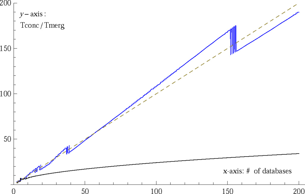Figure 1. Plots for T_con_c/T_merg, for non decreasing and bounded above sequence of database sizes (blue curve), and an unbounded one (black curve). Here the bounded sequence $N_{j} = 2^{b_{j}}$ , $b_{j} = ⌊ \frac{6 j^{2} + j - 1}{j^{2} + 4} ⌋$ ,N₁ = 2, $λ = ⌊ \frac{\frac{π}{4} \sqrt{p}}{\frac{π}{4} \sqrt{q}} ⌋$ ,p = 2⁶, q = N₁ = 2, and the unbounded one N_j = 2^j, N₁ =2 are used. Dashed line: y = x.
of the complexities, we have that $T_{c o n c}^{(c)} / T_{m e r g}^{(c)} = n$ , for all n.
Since every sequence in R has a monotone subsequence, it follows that, given a bounded above sequence {N_j}, we can always extract a monotone subsequence ${N_{c_{j}}}$ necessarily bounded, and therefore convergent. (c.f. Bolzano-Weirstrass theorem, stating that each bounded sequence in R^m has a convergent subsequence). Hence, even if {N_j} is bounded above but not convergent, if using only ${N_{c_{j}}}$ as database sizes, the ratio T_conc/T_merg will be close to database number.
A geometric interpretation of inequalities of the proposition, providing bounds for the complexity, is that asymptotically, the ratio $\frac{T_{c o n c}}{T_{m e r g}}$ lies in the interior of an angle δ = arctan(λ) − arctan(λ⁻¹) with vertex at point (0, 0) and sides along directions nλ⁻¹ and nλ, symmetric wrt bisector y = x; it lies on the bisector if N_i = N, i.e., all distances are equal, (in this case the search operator is $U_{G; c o n c} (n N) = \oplus_{i = 1}^{n} U_{G} (N) = 1_{n} \otimes U_{G} (N))$ .

A special case of minimum complexity is stated in the following lemma.

Lemma 6. The complexity of an l merging is minimum and independent of l if and only if all involved database dimensions are equal.

2.3. Collective Quantum Search: Threshold Cases

Summarizing the study so far by referring to sequences (1ⁿ) ≺ π₂ ≺ … ≺ π_k−1 ≺ (n) and

T_{(1^{n})} \geq T_{π}_{_{2}} \geq \dots \geq T_{π_{k - 1}} \geq T_{(n)}

, we note that: the first sequence concerns the weak ordering of partitions ranging from total concatenation to total merging of n searches. The second one concerns the associated numerical ordering of these schemes via comparison between their corresponding complexities. We seek to clarify which are the generic threshold cases in the sequences according to some criteria, i.e., the cases in which merging gives no computational advantage in search, due to some circumstantial reasons to be determined. Two such criteria are, the conjugate partition criterion (CPC), and the threshold partition criterion (TPC). In case of CPC the ∗ conjugation for partitions is used to single out as threshold cases the self-conjugate partitions π = π^∗ for which T_π = T_π∗, [13], under some specified database dimensions. In case of TPC the threshold cases are the so called threshold partition π, which hold a balanced number of boxes (searches) in the upper and lower parts of its Young diagram.

2.3.1. Conjugate Partition Criterion

The complexity of any joining scheme is determined both by the partition shaping its Young diagram and by filling of partition’s boxes by the respective Hilbert space dimensions N_i of quantum databases. A simplification is the standard tableau and particularly the physically motivated choice N_i = 2ⁱ. Consider n jointed searches interpolating between full concatenation with partition (1ⁿ) and full merging with partition (n). Consider the conjugation of partition π → π^∗, which produces partition π^∗ by turning rows into column and vice versa and then assign dimensions N_ij to each box (search), i.e., (π_i, j) → N_ij, and seeks values for N_ij, so that the ensuing complexities are equal, i.e., T_π = T_π∗. This equality is achieved by any intermediate joining scheme (1ⁿ) ≺ π ≺ (n), which is self conjugate, i.e., π = π^∗. E.g. in π ⊢ 6, partition π = (3, 2, 1) is self-conjugate and the next choice of dimensions gives equal complexity

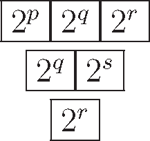
The indicated filling with dimensions p, q, r, s fulfils condition, i.e., T_(3,2,1) = T_(3,2,1)∗.

2.3.2. Threshold Partition Criterion

Proceeding from full concatenation to full merging of n searches by moving up one box at a time (merging one more search), creates diagrams that majorize all preceding ones, as explained. Explicitly, let of division of a Y (π) into two disjoint pieces, Y_u(π) with boxes lying on and to the right of the diagonal, and Y_d(π) be the rest piece, i.e., Y(π) = Y_u(π)∪Y_d(π). E.g. for partition π = (6, 5, 3, 3, 2, 2, 1) the diagrams Y (π), Y_u(π) and Y_d(π) are

Let next y_u(π) be a partition whose parts are the lengths of the rows of the shifted shape Y_u(π), and y_d(π) be the partition whose parts are the lengths of the columns of Y_d(π). If n is even and π ⊢ n, then partition π is called graphic partition iff y (π)^w≺y_d(π) and it is called threshold partition π_th iff y_u(π_th) = y_d(π_th) [13]. In the case of threshold partition it follows that T_yu₍_π₎ = T_yd₍_π₎ and that half of the number of merging responsible for crossing the diagonal have already happened (i.e.,

| y_{u} | = | y_{d} | = \frac{N}{2}

). This threshold relation landmarks the midway situation before the onset of total merging. For the example above the pairs y_u(π) = (6, 4, 1), y_d(π) = (6, 4, 1), and y_u(π) = (7, 3, 1), y_d(π) = (6, 3, 2) satisfy the TPC.

2.4. Oracle Algebra for Collective Quantum Search

Let database Hilbert spaces

H_{N_{1}}

,

H_{N_{2}}

,

H_{N_{3}}

, where

H_{N_{i}} = l_{2} (Δ_{N_{i}})

with N₁ = N₂ = N₃ = 4, and let the marked items be the first, the third, and the second elements in

H_{N_{1}}

,

H_{N_{2}}

,

H_{N_{3}}

, respectively. To the partitions (111), (21), (3), of 3, correspond the joining (i) a 3−merging in database

H_{N_{1} + N_{2} + N_{3}} = \oplus_{i = 1}^{3} H_{N_{i}}

, (ii) a 2-merging in

H_{N_{1} + N_{2}} = \oplus_{i = 1}^{2} H_{N_{i}}

, a single in

H_{N_{3}}

, and concatenation between them, and finally (iii) concatenation of searches in

H_{N_{1}}

,

H_{N_{2}}

,

H_{N_{3}}

. Using notation

| x_{N}^{π} ⟩

and

π_{N} (Σ_{a}^{π})

, a = 1, 2, 3, 0 we have:

3-merging in $H_{N_{1} + N_{2} + N_{3}}$ ;
The marked items are |1⟩, |7⟩, |10⟩, so $| x_{12}^{(3)} ⟩ = \frac{1}{\sqrt{3}} (| 1 ⟩ + | 7 ⟩ + | 10 ⟩)$ , $| x_{12}^{(3)}^{⊥} ⟩ = \frac{1}{\sqrt{9}} (| 2 ⟩ + | 3 ⟩ + | 4 ⟩ + | 5 ⟩ + | 6 ⟩ + | 8 ⟩ + | 9 ⟩ + | 11 ⟩ + | 12 ⟩)$ ,and the 12-dim representation of oracle Ealgebra generators are

$\begin{matrix} π_{12} (Σ_{1}^{(3)}) = π_{12} (| x_{12}^{(3)} ⟩ ⟨ x_{12}^{(3) ⊥} |) + H . c ., π_{12} (Σ_{2}^{(3)}) = π_{12} (- i | x_{12}^{(3)} ⟩ ⟨ x_{12}^{(3) ⊥} |) + H . c ., \\ π_{12} (Σ_{3}^{(3)}) = π_{12} (| x_{12}^{(3)} ⟩ ⟨ x_{12}^{(3)} |) - H . c ., π_{12} (Σ_{0}^{(3)}) = π_{12} (| x_{12}^{(3)} ⟩ ⟨ x_{12}^{(3)} |) + H . c . \end{matrix}$
2-merging in $H_{N_{1} + N_{2}}$ , single search in $H_{N_{3}}$ , and concatenation between them; The marked items are |1⟩, |7⟩ in $H_{N_{1} + N_{2}}$ , and |2⟩ in $H_{N_{3}}$ , so $| x_{8}^{(2, 1)} ⟩ = \frac{1}{\sqrt{2}} (| 1 ⟩ + | 7 ⟩)$ , $| x_{8}^{(2, 1)}^{⊥} ⟩ = \frac{1}{\sqrt{6}} (| 2 ⟩ + | 3 ⟩ + | 4 ⟩ + | 5 ⟩ + | 6 ⟩ + | 8 ⟩)$ , $| x_{4}^{(2, 1)} ⟩ = | 2 ⟩$ , $| x_{4}^{(2, 1) ⊥} ⟩ = \frac{1}{\sqrt{3}} (| 1 ⟩ + | 3 ⟩ + | 4 ⟩)$ . Since e.g., $| x_{12}^{(2, 1)} ⟩ = | x_{8}^{(2, 1)} ⟩ \oplus | x_{4}^{(2, 1)} ⟩$ , the generators decompose

$π_{12} (Σ_{a}^{(2, 1)}) = π_{8} (Σ_{a}^{(2, 1)}) \oplus π_{4} (Σ_{a}^{(2, 1)}) .$
Single searches in $H_{N_{1}}$ , $H_{N_{2}}$ and $H_{N_{3}}$ and concatenation between them;
The marked items are |1⟩, ∈ $H_{N_{1}}$ ,|3⟩ ∈ $H_{N_{2}}$ , and |2⟩ ∈ $H_{N_{3}}$ and |2⟩ ∈. E.g. for $H_{N_{1}}$ , $| x_{4}^{(1, 1, 1)} ⟩ = | 1 ⟩$ , $| x_{4}^{(1, 1, 1) ⊥} ⟩ = \frac{1}{\sqrt{3}} (| 2 ⟩ + | 3 ⟩ + | 4 ⟩)$ , etc, so for a = 1, 2, 3, 0, the following decomposition is obtained,

$π_{12} (Σ_{a}^{(1, 1, 1)}) = \underset{H_{1, 2, 3}}{\oplus} π_{4} (Σ_{a}^{(1, 1, 1)}) .$

Having the oracle algebra matrix generators we compute the unitary search operators for the three corresponding partitions,

\begin{matrix} U_{G}^{(3)} = \exp (i θ_{12} π_{12} (Σ_{2}^{(3)})), \\ U_{G}^{(2, 1)} = \exp (i θ_{8} π_{8} (Σ_{2}^{(2, 1)})) \oplus \exp (i θ_{4} π_{4} (Σ_{2}^{(2, 1)})), \\ U_{G}^{(1, 1, 1)} = \underset{H_{1, 2, 3}}{\oplus} \exp (i θ_{4} π_{4} (Σ_{2}^{(1, 1, 1)})), \end{matrix}

where

θ_{N} = \arcsin (- 2 \sqrt{k (N - k)} / N)

with k = 1. By means of a similar search unitary, the collective quantum search complexity measures can be computed.

2.4.1. Generalized Azimuthal Symmetry

Let the partition τ = (N₁, N₂, ⋯, N_l) of N of length l = l(τ), and let the one parameter subgroup

U_{a} (1) = e^{i ϕ_{a} π_{a} (Σ_{3})}

, generated by π_a(Σ₃) ∈ End(H_a). Let the group G = U(N) and the subgroup

K = \oplus_{a = N_{1}}^{N_{l}} U_{a} (1)

. Consider a concatenation of l searches for a given partition τ ⊢ N, with search operator

U_{G}^{(τ)} : = \oplus_{a = N_{1}}^{N_{l}} U_{G}^{(a)}

and search step implemented by the transformation

ρ \to U_{G}^{(τ)} ρ U_{G}^{(τ) †}

. Let further the unitary operator

V_{3} (ϕ) = \oplus_{a = N_{1}}^{N_{l}} e^{i ϕ_{a} π_{a} (Σ_{3})} \in K

,

ϕ = {(ϕ_{a})}_{a = N_{1}}^{N_{l}} \in {[0, 2 π)}^{l}

then the transformation

ρ \to ρ^{'} = V_{3} (ϕ) U_{G}^{(τ)} ρ U_{G}^{(τ) †} V_{3} {(ϕ)}^{†},

preserves the projection of density matrix ρ along the collective marked vector

| x ⟩ ⟨ x | : = \oplus_{a = N_{1}}^{N_{l}} | x_{a} ⟩ ⟨ x_{a} |

, or equivalently preserves the

\oplus_{a = N_{1}}^{N_{l}} π_{a} (Σ_{3})

component of the collective density matrix [9]. This implies the search complexity remains invariant under the action of V₃.

This equality of complexities is expressed in terms of the minimization of the projection of time-evolved collective density matrix on the collective marked item, i.e.,

\begin{array}{l} 1 = \min_{α} ⟨ x | U_{G}^{(τ) α} ρ_{s s} U_{G}^{(τ) † α} | x ⟩ \\ = \min_{α} ⟨ x | (U_{G}^{(τ) α_{1}} V_{3} (ϕ) U_{G}^{(τ) α_{2}} \dots V_{3} (ϕ) U_{G}^{(τ) α_{r}}) ρ_{s s} \\ \times {(U_{G}^{(τ) α_{1}} V_{3} (ϕ) U_{G}^{(τ) α_{2}} \dots V_{3} (ϕ) U_{G}^{(τ) α_{r}})}^{†} | x ⟩, \end{array}

where α = α₁ + ⋯ + α_r, which is a generalization of an analogues formula for l = 1, describing the azimuthal symmetry of single search algorithm [9]. To any partition τ ⊢ N there corresponds a symmetry group M_τ = G/K for the collective quantum search.

3. Proofs, Examples, and Discussion

In this second part of the paper we have put together a number of items:

“Collective quantum search: Merging and Concatenation”, with proofs of lemmas and numerical examples; in the following section.
“Collective quantum search: Joining Schemes and Young diagrams” we have placed the proof of the main proposition and of the auxiliary lemmas, together with numerical examples that demonstrate the workings of collective quantum search; in the final section.
“Oracle algebra and representations” we introduce the mathematical details of the oracle algebra and some examples from its matrix representations.

3.1. Collective Quantum Search

3.1.1. Merging and Concatenation

Proof. (Lemma 1) The target vector decomposes in

| x_{c o n c} ⟩ = | x_{1} ⟩ \oplus {| \emptyset ⟩}_{N_{2}} + {| \emptyset ⟩}_{N_{1}} \oplus | x_{2} ⟩ \in H_{1} \oplus H_{2}

. Let the initial vectors |x_conc⟩, |s_conc⟩ and the corresponding projection operators |x_conc⟩⟨x_conc|, |s_conc⟩ ⟨s_conc|. Then

\begin{matrix} | s_{c o n c} ⟩ = | s_{1} ⟩ \oplus {| \emptyset ⟩}_{N_{2}} + {| \emptyset ⟩}_{N_{1}} \oplus | s_{2} ⟩ = (\begin{array}{l} | s_{1} ⟩ \\ | s_{2} ⟩ \end{array}) \\ | s_{c o n c} ⟩ ⟨ s_{c o n c} | = (\begin{matrix} | s_{1} ⟩ ⟨ s_{1} | \\ | s_{2} ⟩ ⟨ s_{2} | \end{matrix}) = | s_{1} ⟩ ⟨ s_{1} | \oplus | s_{2} ⟩ ⟨ s_{2} | \\ J_{s_{c o n c}} = 1_{N_{1} + N_{2}} - 2 | s_{c o n c} ⟩ ⟨ s_{c o n c} | = (\begin{matrix} J_{s_{1}} \\ J_{s_{2}} \end{matrix}) = J_{s_{1}} \oplus J_{s_{2}} . \end{matrix}

Similarly

| x_{c o n c} ⟩ ⟨ x_{c o n c} | = | x_{1} ⟩ ⟨ x_{1} | \otimes | x_{2} ⟩ ⟨ x_{2} |

and

J_{x_{c o n c}} = 1_{N_{1} + N_{2}} - 2 | x_{c o n c} ⟩ ⟨ x_{c o n c} | = (\begin{matrix} J_{x_{1}} \\ J_{x_{2}} \end{matrix}) = J_{x_{1}} \oplus J_{x_{2}}

So the search operator by means of the previous decomposition splits into a direct sum, i.e.

U_{c o n c} (f_{c o n c}) = - (J_{s_{1}} \oplus J_{s_{2}}) (J_{x_{1}} \oplus J_{x_{2}}) = U_{1} \oplus U_{2} .

Similarly, for an l-concatenation it is valid that

U_{c o n c} = \oplus_{j = 1}^{l} U_{j} .

□

Symmetries of U_conc and U_merg. For concatenation, the search operator is determined up to a V₁ ⊕ V₂ unitary, i.e.

U_{c o n c} = - (V (N_{1}) \oplus V (N_{2})) (J_{s_{1}} \oplus J_{s_{2}}) {(V (N_{1}) \oplus V (N_{2}))}^{†} (J_{x_{1}} \oplus J_{x_{2}}) .

Note that V(N₁) ⊕ V(N₂) is the diagonal subgroup of group V(N₁ + N₂). By induction on l, a l-concatenation algorithm, has

\oplus_{i = 1}^{l} V

(Nl)-symmetry, which is the diagonal subgroup of U(N_merg).

Grover [2] showed that for a single search algorithm with one target vector, the unitary search operator U_G = −J_sJ_x can be replaced by a more general operator which is also unitary and it can be in one of the two following equivalent forms

\begin{array}{l} U_{G} = - J_{s} V^{†} J_{x} V \\ U_{G} = - V^{†} J_{s} V J_{x}, \end{array}

with V ∈ U(N). These symmetries survive in the case of joined searches as follows. For merged algorithms the unitary symmetry is U(N_merg), i.e.,

U_{m e r g} = - J_{s_{m e r g}} V {(N_{m e r g})}^{†} J_{x_{m e r g}} V (N_{m e r g}) .

3.1.2. Joining Schemes and Young diagrams

Partitions are specified by lower case Greek letters. If λ is a partition of a non negative integer k, we write λ ⊢ k and call k the weight of the partition, and λ = (λ₁, …, λ_k) is a sequence of non negative integers λ_i for i = 1, 2, …, k, such that λ₁ ≥ λ₂ ≥ … ≥ λ ≥ 0 with

\sum_{i = 1}^{k} λ_{i} = k

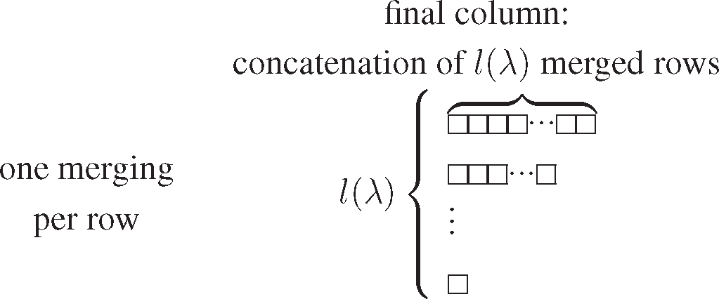
. The non zero λ_i are called the parts of λ and their number l(λ) is the length of λ. In specifying λ, the trailing zeros, that is those λ_i = 0, are often omitted. By way of illustration, if k = 10, we regard (4, 2, 2, 1, 1, 0, 0, 0, 0, 0) and (4, 2, 2, 1, 1) as the same partition λ, for which it holds that |λ| = 10 and l(λ) = 5. Each partition λ of weight |λ| = k, and length l(λ) defines a (Ferrers) Young diagram Y (λ) consisting of |λ| boxes arranged in l(λ) left-adjusted rows of lengths from top to bottom λ₁, …, λ_l_(λ), while zeros in λ do not appear in Y (λ) (in the English convention). The notation follows in large part that of [11].

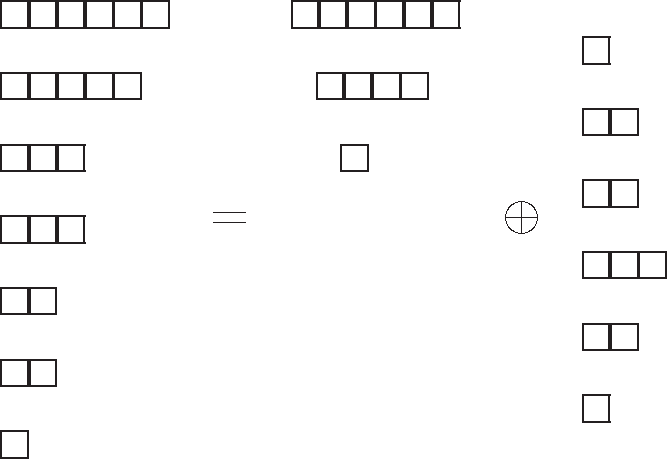
The notion of number partition is associated to the joining of quantum searches as follows: given a number of search algorithms m with database dimensions N₁, N₂, …, N_m, we can join them either by merging or by concatenating in various ways therefore number m is partitioned as λ ⊢ m, where every part λ_i of λ denotes the number of algorithms joined in a similar way, i.e., either by merging or by concatenation. Thus every possible joining scheme corresponds to a Ferrers diagram and vice versa, i.e., π → T_π, ρ → T_ρ, we find by way of example that T_π ≤ T_ρ.

The latter implies that the sequence of majorized partitions is mapped to the multi-set of complexities, i.e., the example of partitions of 6 worked out below yields

\begin{array}{l} π ⊢ 6 : 6 ≻ 51 ≻ 42 ≻ \frac{3^{2}}{41^{2}} ≻ 321 ≻ \frac{2^{3}}{31^{3}} ≻ 2^{2} 1^{2} ≻ 21^{4} ≻ 1^{6} \\ T_{π} : 3 < 4 < 6 \leq \frac{6}{7} < 9 \leq \frac{9}{10} < 12 < 14 < 17 \end{array}

The multi-set of complexities {3, 4, 6, 6, 7, 9, 9, 10, 12, 14, 17} form a piecewise ordered set where the numerical ordering is anti-isotonic wrt the majorization order i.e., in general π ≻ ρ corresponds to T_π ≤ T_ρ. See Figure 2 below.

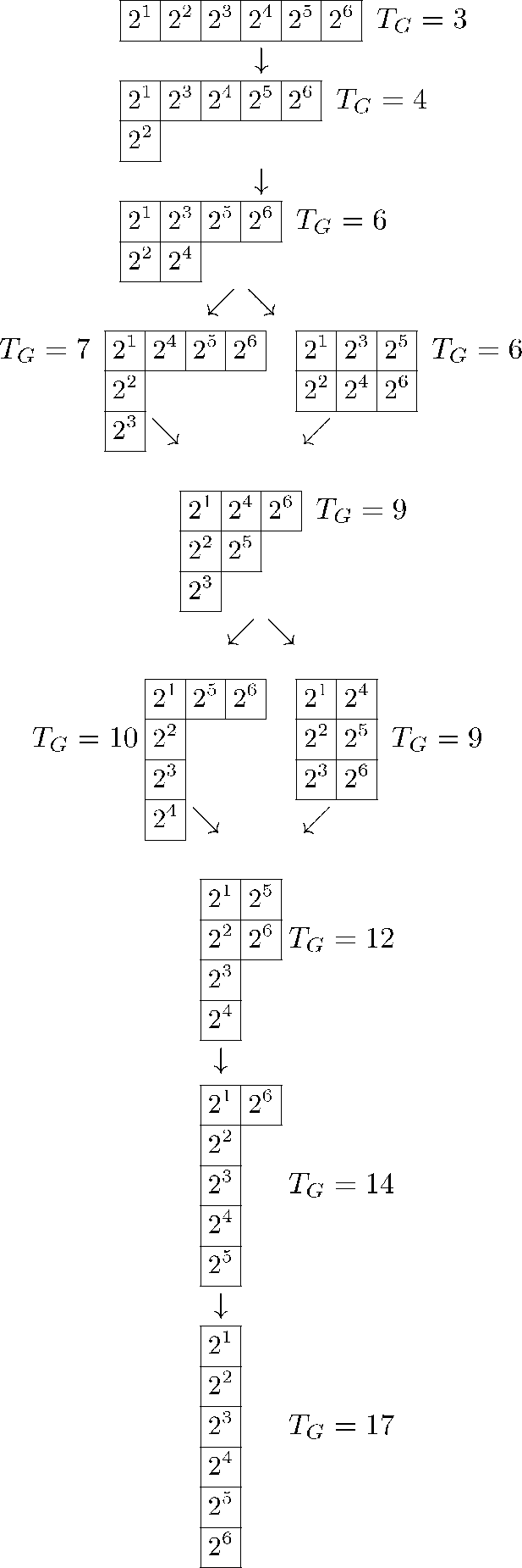
Figure 2. Young tableaux for m = 6 and the corresponding complexities T_G.

3.1.3. Complexity

Proof. (Lemma 3) Let an integer partition π = (π₁, …, π_j, …, π_l₍_π₎) ⊢ n, and the multi-variable functions

ϕ_{μ} (x) : R_{+}^{n} \to R

, µ = 1, 2, …, l(π), where

ϕ_{μ} (x) = ⌊ \frac{π}{4} \frac{1}{\sqrt{π_{μ}}} \sqrt{\sum_{j = 1}^{π_{μ}} x_{j}} ⌋,

with x = (x₁, …, x_n), and π_i the part i of partition π, which enumerates the number of databases involved in a merging scheme. Each of these functions ϕ_µ is a multi-variable Schur-concave function: indeed since

(x, y) \to \sqrt{x + y}

is Schur-concave function and also x → ⌊ϕ(x)⌋ is a Schur-concave function if ϕ(x) is one (Chapter 3 in [10]), we conclude that ϕ_µ as well as their linear combination is a Schur-concave function.

The linear combination of ϕ_µ’s functions is also a Schur-concave function, and this in particular is valid for the search complexity T_π associated with a partition π, i.e., π → T_π, or explicitly

T_{π} (x) = \sum_{μ = 1}^{l_{(π)}} ϕ_{μ} (x) .

is Schur-concave.

So, if π, ρ ⊢ t s.t. π ≻ ρ, then T_π(N) ≤ T_ρ(N), where N = (N₁, …, N_t) □

Diagrammatically

\begin{matrix} π ≻ ρ \\ ↓ ↓ \\ T_{π} \leq T_{ρ} \end{matrix}

Example 1. For n = 16 and the partition π = (6, 4, 4, 2), there are four functions of variables x = (x₁, …, x₁₆),

\begin{array}{l} ϕ_{1} (x_{1}, \dots, x_{16}) = ⌊ \frac{π}{4 \sqrt{6}} \sqrt{x_{1} + x_{2} + x_{3} + x_{4} + x_{5} + x_{6}} ⌋, \\ ϕ_{2} (x_{1}, \dots, x_{16}) = ⌊ \frac{π}{4 \sqrt{4}} \sqrt{x_{7} + x_{8} + x_{9} + x_{10}} ⌋, \\ ϕ_{3} (x_{1}, \dots, x_{16}) = ⌊ \frac{π}{4 \sqrt{4}} \sqrt{x_{11} + x_{12} + x_{13} + x_{14}} ⌋, \\ ϕ_{4} (x_{1}, \dots, x_{16}) = ⌊ \frac{π}{4 \sqrt{2}} \sqrt{x_{15} + x_{16}} ⌋ . \end{array}

each one of them and their linear combination is a Schur-concave function.

Proof. (Lemma 4) Applying Jensen inequality [14] for the convex function

x \to \sqrt{x}

yields

\frac{π}{4} \sqrt{\frac{N_{1} + \dots + N_{l}}{l}} \leq \frac{1}{l} (\frac{π}{4} \sqrt{N_{1}} + \dots + \frac{π}{4} \sqrt{N_{l}})

which implies

⌊ \frac{π}{4} \sqrt{\frac{N_{1} + \dots + N_{l}}{l}} ⌋ \leq ⌊ \frac{π}{4} \sqrt{N_{1}} ⌋ + \dots + ⌊ \frac{π}{4} \sqrt{N_{l}} ⌋ .

In the relation above the equality is reached iff

0 \leq \sum_{i = 1}^{l} {\frac{π}{4} \sqrt{N_{i}}} < \frac{1}{2}

, where {x} denotes the fractional part of the real number x. Notice that the special case where all the numbers appearing in the integral part are all integers, never occurs due to the involvement of π. □

Proof. (Lemma 6) Let N₁, …, N_l be the sizes of databases, then the complexity equals

T_{m e r g}^{(N_{1}, \dots, N_{l})} = ⌊ \frac{π}{4} \sqrt{\frac{N_{1} + \dots + N_{l}}{l}} ⌋ .

Due to AM-GM inequality, we take that

T_{m e r g}^{(N_{1}, \dots, N_{l})} \geq ⌊ \frac{π}{4} \sqrt{\sqrt[l]{N_{1} \dots N_{l}}} ⌋ = ⌊ \frac{π}{4} \sqrt[2 l]{N_{1} \dots N_{l}} ⌋

The equality holds iff N₁ = … = N_l ≡ N, and therefore the minimum is

T_{m e r g, \min}^{(N, \dots, N)} = ⌊ \frac{π}{4} \sqrt{N} ⌋ .

Remark 2.

For comparison reasons we find that the complexity of l-concatenation algorithm is

$T_{c o n c}^{(N_{1}, \dots, N_{l})} = \sum_{j = 1}^{l} ⌊ \frac{π}{4} \sqrt{N_{j}} ⌋$

since $U_{c o n c} = \oplus U_{j} (f_{j})$ . Moreover, if N₁ = … = N_l ≡ N, then

$T_{c o n c}^{(N, \dots, N)} = l ⌊ \frac{π}{4} \sqrt{N_{j}} ⌋ = l T_{m e r g, \min}^{(N, \dots, N)},$
The total tableau complexity for a joining scheme described by its corresponding Young diagram λ is computed as follows: let a Young diagram λ = (i₁, i₂, …, i_r) then the total search algorithm consists of r groups of concatenated sub-algorithms where each group contains i₁, i₂, …, i_r merged algorithms. Via previous lemma and remark, the tableau complexity equals $T_{λ}^{(N_{1}, \dots, N_{k})} = ⌊ \frac{π}{4} \sqrt{\frac{N_{1} + \dots + N_{i_{1}}}{i_{1}}} ⌋ + ⌊ \frac{π}{4} \sqrt{\frac{N_{i_{1} + 1} + \dots + N_{i_{1} + i_{2}}}{i_{2}}} ⌋ + \dots + ⌊ \frac{π}{4} \sqrt{\frac{N_{i_{1} + \dots + i_{r - 1} + 1} + \dots + N_{k}}{i_{r}}} ⌋$ , where i₀ = 0 and i₁ +⋯+ i_r = k. If all databases are of equal size N, then for any diagram λ the tableau complexity equals $T_{λ}^{(N, \dots, N)} = r ⌊ \frac{π}{4} \sqrt{N} ⌋$ .

3.1.4. Main Proposition

Next, we consider the ratio of the extreme values of complexities T_conc/T_merg (“all concatenated” over “all merged”), and regarding the sequence of the dimensions

{N_{i}}_{i = 1}^{n}

, two cases are arising for its asymptotic behaviour. Moreover, for arbitrary positive integers (database sizes) N_i, i = 1, 2, …, n we prove that for the continuous analogues (continuous functions) for the complexities T_conc, T_merg, it holds that

\sqrt{n} < \frac{T_{c o n c}^{(c)}}{T_{m e r g}^{(c)}} \leq n

.

In more details, if

{N_{i}}_{i = 1}^{n}

is an unbounded sequence, specifically N_i’s are consecutive terms of the geometric sequence 2ⁱ (which is the most natural and reasonable choice for database sizes), we conclude that

T_{c o n c} / T_{m e r g} = O (\sqrt{n})

. Otherwise, namely if the sequence

{N_{i}}_{i = 1}^{n}

is bounded (e.g.,

N_{i} = 2^{b_{i}}

, where

{b_{i}}_{i = 1}^{n}

is bounded), it results that the ratio T_conc/T_merg is asymptotically linear with respect to the number n of the databases. This fact leads to an interesting observation: although the qualitative difference between a bounded and an unbounded sequence of database sizes is essential (notice that N_i = 2ⁱ increases exponentially fast), however, the quantitative change that entails to the ratio of complexities, is only quadratic (quadratic reduction) with respect to the database population.

Proof. (Lemma 5) Straightforward calculations. □

Proposition 2. For arbitrary positive integers (database sizes) N_i, i = 1, 2, …, n it holds that

\sqrt{n} T_{m e r g}^{(c)} < T_{c o n c}^{(c)} \leq n T_{m e r g}^{(c)}

Moreover, if N_i are:

consecutive terms of the unbounded sequence ${N_{i}}_{i = 1}^{n}$ with N_i = 2ⁱ, then $T_{c o n c} = O (\sqrt{n}) T_{m e r g}$
terms of a bounded sequence of positive integers with $p = \sup {N_{i}}_{i = 1}^{n}$ , $q = \inf {N_{i}}_{i = 1}^{n}$ , $t h e n : \frac{T_{c o n c}}{T_{m e r g}} \in Θ (n)$ , i.e., nλ⁻¹T_merg ≤ T_conc ≤ nλT_merg, with $λ = ⌊ \frac{π}{4} \sqrt{p} ⌋ {⌊ \frac{π}{4} \sqrt{q} ⌋}^{- 1}$ .

Proof. Applying the Cauchy-Schwarz inequality we obtain that:

T_{c o n c}^{(c) 2} \leq n^{2} T_{m e r g}^{(c) 2}

. Moreover

T_{c o n c}^{(c)} = \sum_{i = 1}^{n} \frac{π}{4} \sqrt{N_{i}} > \frac{π}{4} \sqrt{\sum_{i = 1}^{n} N_{i}} = T_{m e r g}^{(c)} \sqrt{n}

, so

\sqrt{n} < \frac{T_{c o n c}^{(c)}}{T_{c o n c}^{(c)}}

.

Carrying out trivial calculations, we take :

$\frac{1}{n} {(\frac{T_{c o n c}^{(c)}}{T_{m e r g}^{(c)}})}^{2} = 1 + \frac{2 \sum_{i \neq j} \sqrt{N_{i} N_{j}}}{T_{m e r g}^{(c) 2}} \frac{π^{2}}{16 n} .$

In this first case, we have that N_i = 2ⁱ, so

$2 \sum_{i \neq j} \sqrt{N_{i} N_{j}} = 2 {(\sqrt{2 n} - 1)}^{2} {(\sqrt{2} + 1)}^{2} - 2 (2^{n} - 1)$

and $T_{m e r g}^{(c) 2} = \frac{π^{2}}{16 n} 2 (2^{n} - 1)$ . Therefore:

$\frac{1}{n} {(\frac{T_{c o n c}^{(c)}}{T_{m e r g}^{(c)}})}^{2} = \frac{{(1 - \frac{1}{\sqrt{2^{n}}})}^{2} {(\sqrt{2} + 1)}^{2}}{1 - \frac{1}{2^{n}}} .$

The RHS of the above asymptotically equals to ${(\sqrt{2} + 1)}^{2}$ , so $\frac{T_{c o n c}^{(c)}}{T_{m e r g}^{(c)}} \approx (\sqrt{2} + 1) \sqrt{n}$ , i.e. $\frac{T_{c o n c}^{(c)}}{T_{m e r g}^{(c)}} = O (\sqrt{n})$ and $\frac{T_{c o n c}}{T_{m e r g}} = O (\sqrt{n})$ because due to previous Lemma and

$\lim_{n \to \infty} \frac{n}{T_{m e r g}^{(c)}} = 0, T_{m e r g}^{(c)} ≫ 1$

asymptotically, it holds that

$\frac{T_{c o n c}}{T_{m e r g}} \approx \frac{T_{c o n c}^{(c)}}{T_{m e r g}^{(c)}} .$
Since $p = \sup {N_{i}}_{i = 1}^{n}$ , $q = \inf {N_{i}}_{i = 1}^{n}$ , then for all i = 1, 2, …, n, is valid that 2 ≤ q ≤ N_i ≤ p, so

$n ⌊ \frac{π}{4} \sqrt{q} ⌋ \leq T_{c o n c} = \sum_{i = 1}^{n} ⌊ \frac{π}{4} \sqrt{N_{i}} ⌋ \leq n ⌊ \frac{π}{4} \sqrt{p} ⌋ .$

Moreover $⌊ \frac{π}{4} \sqrt{q} ⌋ \leq T_{m e r g} \leq ⌊ \frac{π}{4} \sqrt{p} ⌋$ . Therefore $n λ^{- 1} \leq \frac{T_{c o n c}}{T_{m e r g}} \leq n λ$ and $\frac{T_{c o n c}}{T_{m e r g}} \in Θ (n)$ . □

3.1.5. Geometry of Complexity Reduction

All concave functions fulfil a very intuitive geometric condition with their graph, namely that the center of mass of a set of points lying on the graph is lying not above the graph itself. Quantifying this geometric property leads to the Jensen inequality [14], which in fact is the reason for achieving complexity reduction in various forms of joining schemes. This is demonstrated below by means of a numerical example.

Example 2. Numerical example (see Figure 3). Let the Young diagram of shape (5, 4, 1) and let the following Young tableau (strictly increasing row and column-wise, no repetitions)

where N_i’s are database sizes : N₁ = 2³, N₂ = 2⁴, N₃ = 2⁵, N₄ = 2⁶, N₅ = 2⁷, N₆ = 2⁸, N₇ = 2⁹, N₈ =2¹⁰, N₉ = 2¹¹, N₁₀ = 2¹²

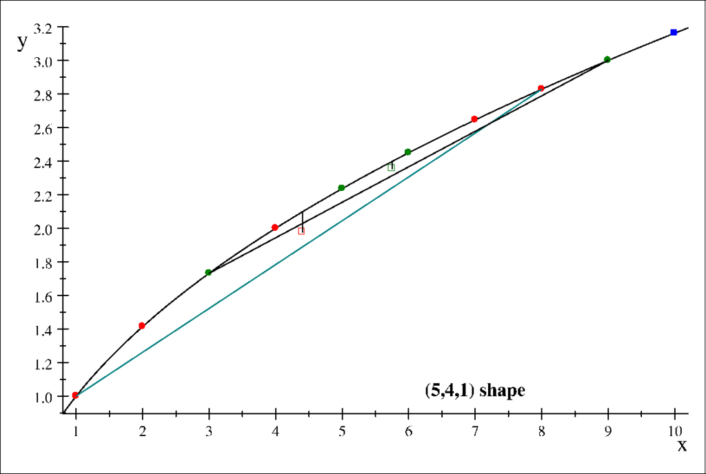
Figure 3. Jensen’s inequality for the numerical example. Round dots represent points lying on the graph, and square dots represent center of mass points.

Row 1

Referring to the graph of the complexity function

y = f (x) = \sqrt{x}

we mark the 5 points

n^{1} = {(2^{3}, \sqrt{2^{3}}), (2^{4}, \sqrt{2^{4}}), (2^{6}, \sqrt{2^{6}}), (2^{9}, \sqrt{2^{9}}), (2^{10}, \sqrt{2^{10}})}

and the center of mass vector c¹, with coordinates

(\frac{2^{3} + 2^{4} + 2^{6} + 2^{9} + 2^{10}}{5}, \frac{\sqrt{2^{3}} + \sqrt{2^{4}} + \sqrt{2^{6}} + \sqrt{2^{9}} + \sqrt{2^{10}}}{5}) = (324.8, 13.891)

and its crossing point with the graph of

f : q^{1} = (324.8, \sqrt{324.8}) = (324.8, 18.0222)

.

Row 2

In the graph of complexity function

f (x) = \sqrt{x}

mark the 4 points

v^{2} = {(2^{5}, \sqrt{2^{5}}), (2^{7}, \sqrt{2^{7}}), (2^{8}, \sqrt{2^{8}}), (2^{11}, \sqrt{2^{11}})}

the center of mass vector c² = (616.0, 19.556) and its crossing point with the graph

q^{2} = (616.0, \sqrt{616.0,}) = (616.0, 24.8193)

.

Row 3

In the graph of complexity function

f (x) = \sqrt{x}

mark the 1 point v³ = c³ = q³ = (2¹², 2⁶).

Equal Complexity Tableaux and Shapes

Motivated by the geometric explanation of the complexity measure for various schemes of joining quantum search algorithms as has been studied in previous section, we proceed to address the problem of determining shapes and tableaux describing ways of joining searches. We study joining of database spaces of equal dimension N. The complexity is differentiated from one scheme to the other due to the difference of the associated Young diagram shapes, so we call it shape complexity.

\begin{matrix} \begin{matrix} 2 \\ 11 \end{matrix} & \begin{matrix} 3 \\ 21 \\ 111 \end{matrix} & \begin{matrix} 4 \\ 31 \\ 22 \\ 211 \\ 1111 \end{matrix} & \begin{matrix} 5 \\ 41 \\ 32 \\ 311 \\ 221 \\ 2111 \\ 11111 \end{matrix} & \begin{matrix} 6 \\ 51 \\ 42 \\ 411 \\ 33 \\ 321 \\ 3111 \\ 222 \\ 2211 \\ 21111 \\ 111111 \end{matrix} & \begin{matrix} 7 \\ 61 \\ 52 \\ 43 \\ 511 \\ 421 \\ 331 \\ 4111 \\ 322 \\ 3211 \\ 2221 \\ 31111 \\ 22111 \\ 211111 \\ 1111111 \end{matrix} \end{matrix}

Joined quantum searches, all of which have equal Hilbert space dimension N and share the same shape complexity, are displayed as a pattern of bold typed integer partitions from 3 to 7 within the Young lattice. The pattern of equal complexities is independent from N.

c_{y}^{1} + c_{y}^{2} + c_{y}^{3} \leq q_{y}^{1} + q_{y}^{2} + q_{y}^{3}

Figure 4 displays the contour of equal complexity families of joined quantum algorithms having unequal database sizes. A constant complexity difference (vertical segments) is chosen between tableau complexity (lower broken line) describing concatenation of groups of merged quantum searches and its upper bound (upper full line) describing the same group jointed by concatenation only.

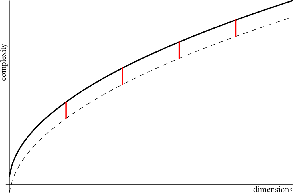
Figure 4. Display of the contour of equal complexity families of joined quantum algorithms. 4. Oracle Algebra and Representations

Definition 2 Let the set Δ = {1, 2, …N}, a subset I ⊂ Δ, and the oracle function f, be the characteristic function of I with k elements, defined as f(i) = 1, for i ∈ I, and f(i) = 0, for i ∉ I. We define as the matrix oracle algebra A_f with respect to the characteristic function f of I ⊂ Δ, the set A_f = {A : A = αΣ₀(f) + βΣ₁(f) + γΣ₂(f) + δΣ₃(f)} where α, β, γ, δ ∈ R are arbitrary real [9,15].

Let also (a) the Hilbert space l₂(D), the vector

| x ⟩ = \frac{1}{\sqrt{k}} \sum_{i = 1}^{N} f (i) | i ⟩,

and its orthogonal vector

| x^{⊥} ⟩ = \frac{1}{\sqrt{N - k}} \sum_{i = 1}^{N} (1 - f (i)) | i ⟩,

with

k = \sum_{i = 1}^{N} f (i)

.

(b) the Hilbert space

H_{N} = s p a n {| i ⟩}_{i = 1}^{N}

, the matrix

{({\hat{1}}_{s t})}_{i j} = 1

, 1 ≤ i ≤ s, 1 ≤ j ≤ t, and the N dimensional matrix representation π_N : A_f → Lin(H_N).

Next, we introduce the following Σ₀, Σ₁, Σ₂, Σ₃, as the generators of A_f :

\begin{array}{l} \sum_{1} = | x ⟩ ⟨ x^{⊥} | + | x^{⊥} ⟩ ⟨ x |, \\ \sum_{2} = - i | | x ⟩ ⟨ x^{⊥} | + i | | x^{⊥} ⟩ ⟨ x |, \\ \sum_{3} = | x ⟩ ⟨ x | - | x^{⊥} ⟩ ⟨ x^{⊥} |, \\ \sum_{0} = | x ⟩ ⟨ x | - | x^{⊥} ⟩ ⟨ x^{⊥} | . \end{array}

For the oracle function f(i) = 1, 1 ≤ i ≤ k < N, and zero otherwise, the representation above reads

\begin{array}{r} π_{N} (\sum_{0}) = (\begin{matrix} \frac{1}{k} {\hat{1}}_{k \times k} & O_{k \times (N - k)} \\ O_{(N - k) \times k} & \frac{1}{N - k} {\hat{1}}_{(N - k) \times (N - k)} \end{matrix}), \\ π_{N} (\sum_{1}) = (\begin{matrix} O_{k \times k} & \frac{1}{\sqrt{k (N - k)}} {\hat{1}}_{k \times (N - k)} \\ \frac{1}{\sqrt{k (N - k)}} {\hat{1}}_{(N - k) \times k} & O_{(N - k) \times (N - k)} \end{matrix}), \\ π_{N} (\sum_{3}) = (\begin{matrix} \frac{1}{k} {\hat{1}}_{k \times k} & O_{k \times (N - k)} \\ O_{(N - k) \times k} & - \frac{1}{N - k} {\hat{1}}_{(N - k) \times (N - k)} \end{matrix}), \end{array}

and therefore, for an arbitrary element A ∈ A_f, it holds that

\begin{matrix} π_{N} (\sum_{2}) = (\begin{matrix} O_{k \times k} & - i \frac{1}{\sqrt{k (N - k)}} {\hat{1}}_{k \times (N - k)} \\ i \frac{1}{\sqrt{k (N - k)}} {\hat{1}}_{(N - k) \times k} & O_{(N - k) \times (N - k)} \end{matrix}), \\ π_{N} (α \sum_{0} + β \sum_{1} + γ \sum_{2} + δ \sum_{3}) = (\begin{matrix} \frac{α + δ}{k} {\hat{1}}_{k \times k} & \frac{β + i γ}{\sqrt{k (N - k)}} {\hat{1}}_{k \times (N - k)} \\ \frac{β + i γ}{\sqrt{k (N - k)}} {\hat{1}}_{(N - k) \times k} & \frac{α + δ}{N - k} {\hat{1}}_{(N - k) \times (N - k)} \end{matrix}) . \end{matrix}

4.1. Examples

Show cases: Here we show explicitly the vectors and matrices involved in the possible scenarios of joining via merging and/or concatenation for the specific example of three 4-dimensional quantum searches. Let databases

Δ_{N_{1}}

,

Δ_{N_{2}}

,

Δ_{N_{3}}

, with N₁ = N₂ = N₃ = 4, and let the market items be the first, the third, and the second elements in

Δ_{N_{1}}

,

Δ_{N_{2}}

,

Δ_{N_{3}}

respectively, i.e., |1⟩, |7⟩, |10⟩ in

Δ_{N_{1} + N_{2} + N_{3}}

. The three partitions of 3 are 1 + 1 + 1 = 2 + 1 = 3, we have three possible joining, i.e., (i) a 3−merging in database

Δ_{N_{1} + N_{2} + N_{3}}

, (ii) a 2-merging in

Δ_{N_{1} + N_{2}}

, a single in

Δ_{N_{3}}

, and a concatenation, and finally (iii) three single searches in

Δ_{N_{1}}

,

Δ_{N_{2}}

,

Δ_{N_{3}}

. We use the symbol • to denote non zero matrix elements, and · for zeros.

4.1.1. 3-Merging $Δ_{N_{1} + N_{2} + N_{3}}$

The marked items are |1⟩, |7⟩, |10⟩, so

| x_{12}^{(3)} ⟩ = \frac{1}{\sqrt{3}} (| 1 ⟩ + | 7 ⟩ + | 10 ⟩)

,

| x_{12}^{(3) ⊥} ⟩ = \frac{1}{\sqrt{9}} (| 2 ⟩ + | 3 ⟩ + | 4 ⟩ + | 5 ⟩ + | 6 ⟩ + | 8 ⟩ + | 9 ⟩ + | 11 ⟩ + | 12 ⟩)

, Therefore,

\begin{array}{l} | x_{12}^{(x)} ⟩ = {(\frac{1}{\sqrt{3}}, 0, 0, 0, 0, 0, \frac{1}{\sqrt{3}}, 0, 0, \frac{1}{\sqrt{3}}, 0, 0)}^{T}, \\ | x_{12}^{(x) ⊥} ⟩ = {(0, \frac{1}{\sqrt{9}}, \frac{1}{\sqrt{9}}, \frac{1}{\sqrt{9}}, \frac{1}{\sqrt{9}}, \frac{1}{\sqrt{9}}, 0, \frac{1}{\sqrt{9}}, \frac{1}{\sqrt{9}}, 0, \frac{1}{\sqrt{9}}, \frac{1}{\sqrt{9}})}^{T}, \\ π_{12} (| x_{12}^{(3) ⊥} ⟩ ⟨ x_{12}^{(3)} |) = (\begin{array}{l} \cdot & \cdot & \cdot \\ • & \cdot & \cdot & \cdot & \cdot & \cdot & • & \cdot & \cdot & • & \cdot & \cdot \\ • & \cdot & \cdot & \cdot & \cdot & \cdot & • & \cdot & \cdot & • & \cdot & \cdot \\ • & \cdot & \cdot & \cdot & \cdot & \cdot & • & \cdot & \cdot & • & \cdot & \cdot \\ • & \cdot & \cdot & \cdot & \cdot & \cdot & • & \cdot & \cdot & • & \cdot & \cdot \\ • & \cdot & \cdot & \cdot & \cdot & \cdot & • & \cdot & \cdot & • & \cdot & \cdot \\ \cdot & \cdot & \cdot \\ • & \cdot & \cdot & \cdot & \cdot & \cdot & • & \cdot & \cdot & • & \cdot & \cdot \\ • & \cdot & \cdot & \cdot & \cdot & \cdot & • & \cdot & \cdot & • & \cdot & \cdot \\ \cdot & \cdot & \cdot \\ • & \cdot & \cdot & \cdot & \cdot & \cdot & • & \cdot & \cdot & • & \cdot & \cdot \\ • & \cdot & \cdot & \cdot & \cdot & \cdot & • & \cdot & \cdot & • & \cdot & \cdot \end{array}), \\ π_{12} (| x_{12}^{(3)} ⟩ ⟨ x_{12}^{(3)} |) = (\begin{array}{l} • & \cdot & \cdot & \cdot & \cdot & \cdot & • & \cdot & \cdot & • & \cdot & \cdot \\ \cdot & \cdot & \cdot \\ \cdot & \cdot & \cdot \\ \cdot & \cdot & \cdot \\ \cdot & \cdot & \cdot \\ \cdot & \cdot & \cdot \\ • & \cdot & \cdot & \cdot & \cdot & \cdot & • & \cdot & \cdot & • & \cdot & \cdot \\ \cdot & \cdot & \cdot \\ \cdot & \cdot & \cdot \\ • & \cdot & \cdot & \cdot & \cdot & \cdot & • & \cdot & \cdot & • & \cdot & \cdot \\ \cdot & \cdot & \cdot \\ \cdot & \cdot & \cdot \end{array}), \\ π_{12} (| x_{12}^{(3) ⊥} ⟩ ⟨ x_{12}^{(3) ⊥} |) = (\begin{array}{l} \cdot & \cdot & \cdot & \cdot & \cdot & \cdot & \cdot & \cdot & \cdot \\ \cdot & • & • & • & • & • & \cdot & • & • & \cdot & • & • \\ \cdot & • & • & • & • & • & \cdot & • & • & \cdot & • & • \\ \cdot & • & • & • & • & • & \cdot & • & • & \cdot & • & • \\ \cdot & • & • & • & • & • & \cdot & • & • & \cdot & • & • \\ \cdot & • & • & • & • & • & \cdot & • & • & \cdot & • & • \\ \cdot & \cdot & \cdot & \cdot & \cdot & \cdot & \cdot & \cdot & \cdot \\ \cdot & • & • & • & • & • & \cdot & • & • & \cdot & • & • \\ \cdot & • & • & • & • & • & \cdot & • & • & \cdot & • & • \\ \cdot & \cdot & \cdot & \cdot & \cdot & \cdot & \cdot & \cdot & \cdot \\ \cdot & • & • & • & • & • & \cdot & • & • & \cdot & • & • \\ \cdot & • & • & • & • & • & \cdot & • & • & \cdot & • & • \end{array}) \end{array}

Therefore, the generators of A_f are:

\begin{array}{l} π_{12} (\sum_{1}^{(3)}) = π_{12} (| x_{12}^{(3)} ⟩ ⟨ x_{12}^{(3) ⊥} |) + H . c ., \\ π_{12} (\sum_{2}^{(3)}) = π_{12} (- i | x_{12}^{(3)} ⟩ ⟨ x_{12}^{(3) ⊥} |) + H . c ., \\ π_{12} (\sum_{3}^{(3)}) = π_{12} (| x_{12}^{(3)} ⟩ ⟨ x_{12}^{(3)} |) - π_{12} (| x_{12}^{(3) ⊥} ⟩ ⟨ x_{12}^{(3) ⊥} |), \\ π_{12} (\sum_{0}^{(3)}) = π_{12} (| x_{12}^{(3)} ⟩ ⟨ x_{12}^{(3)} |) + π_{12} (| x_{12}^{(3) ⊥} ⟩ ⟨ x_{12}^{(3) ⊥} |) . \end{array}

4.1.2. 2-Merging $Δ_{N_{1} + N_{2}}$ , single $Δ_{N_{3}}$ , and Concatenation

The marked items are |1⟩, |7⟩ in

Δ_{N_{1} + N_{2}}

, and |2⟩ in

Δ_{N_{3}}

, so

\begin{array}{l} | x_{8}^{(2, 1)} ⟩ = \frac{1}{\sqrt{2}} (| 1 ⟩ + | 7 ⟩) = {(\frac{1}{\sqrt{2}}, 0, 0, 0, 0, 0, \frac{1}{\sqrt{2}}, 0)}^{T}, \\ | x_{8}^{(2, 1) ⊥} ⟩ = \frac{1}{\sqrt{6}} (| 2 ⟩ + | 3 ⟩ + | 4 ⟩ + | 5 ⟩ + | 6 ⟩ + | 8 ⟩) = {(0, \frac{1}{\sqrt{6}}, \frac{1}{\sqrt{6}}, \frac{1}{\sqrt{6}}, \frac{1}{\sqrt{6}}, \frac{1}{\sqrt{6}}, 0, \frac{1}{\sqrt{6}})}^{T}, \\ | x_{4}^{(2, 1)} ⟩ = | 2 ⟩ = {(0, 1, 0, 0)}^{T}, | x_{4}^{(2, 1) ⊥} ⟩ = \frac{1}{\sqrt{3}} (| 1 ⟩ + | 3 ⟩ + | 4 ⟩) = {(\frac{1}{\sqrt{3}}, 0, \frac{1}{\sqrt{3}}, \frac{1}{\sqrt{3}})}^{T}, \end{array}

and

| x_{12}^{(2, 1)} ⟩ = {(\frac{1}{\sqrt{2}}, 0, 0, 0, 0, 0, \frac{1}{\sqrt{2}}, 0, 0, 1, 0, 0)}^{T},

| x_{12}^{(2, 1) ⊥} ⟩ = {(0, \frac{1}{\sqrt{6}}, \frac{1}{\sqrt{6}}, \frac{1}{\sqrt{6}}, \frac{1}{\sqrt{6}}, \frac{1}{\sqrt{6}}, 0, \frac{1}{\sqrt{6}}, \frac{1}{\sqrt{3}}, 0, \frac{1}{\sqrt{3}}, \frac{1}{\sqrt{3}})}^{T},

\begin{array}{l} π_{8} (| x_{8}^{(2, 1) ⊥} ⟩ ⟨ x_{8}^{(2, 1)} |) = (\begin{array}{l} \cdot & \cdot \\ • & \cdot & \cdot & \cdot & \cdot & \cdot & • & \cdot \\ • & \cdot & \cdot & \cdot & \cdot & \cdot & • & \cdot \\ • & \cdot & \cdot & \cdot & \cdot & \cdot & • & \cdot \\ • & \cdot & \cdot & \cdot & \cdot & \cdot & • & \cdot \\ • & \cdot & \cdot & \cdot & \cdot & \cdot & • & \cdot \\ \cdot & \cdot \\ • & \cdot & \cdot & \cdot & \cdot & \cdot & • & \cdot \end{array}), \\ π_{8} (| x_{8}^{(2, 1)} ⟩ ⟨ x_{8}^{(2, 1)} |) = (\begin{array}{l} • & \cdot & \cdot & \cdot & \cdot & \cdot & • & \cdot \\ \cdot & \cdot \\ \cdot & \cdot \\ \cdot & \cdot \\ \cdot & \cdot \\ \cdot & \cdot \\ • & \cdot & \cdot & \cdot & \cdot & \cdot & • & \cdot \\ \cdot & \cdot \end{array}) \\ π_{8} (| x_{8}^{(2, 1) ⊥} ⟩ ⟨ x_{8}^{(2, 1) ⊥} |) = (\begin{array}{l} \cdot & \cdot & \cdot & \cdot & \cdot & \cdot \\ \cdot & • & • & • & • & • & \cdot & • \\ \cdot & • & • & • & • & • & \cdot & • \\ \cdot & • & • & • & • & • & \cdot & • \\ \cdot & • & • & • & • & • & \cdot & • \\ \cdot & • & • & • & • & • & \cdot & • \\ \cdot & \cdot & \cdot & \cdot & \cdot & \cdot \\ \cdot & • & • & • & • & • & \cdot & • \end{array}) \end{array}

Single

Δ_{N_{3}}

\begin{array}{l} π_{4} (| x_{4}^{(2, 1) ⊥} ⟩ ⟨ x_{4}^{(2, 1)} |) = (\begin{array}{l} \cdot & • & \cdot & \cdot \\ \cdot \\ \cdot & • & \cdot & \cdot \\ \cdot & • & \cdot & \cdot \end{array}), \\ π_{4} (| x_{4}^{(2, 1)} ⟩ ⟨ x_{4}^{(2, 1)} |) = (\begin{array}{l} \cdot \\ \cdot & • & \cdot & \cdot \\ \cdot \\ \cdot \end{array}) \\ π_{4} (| x_{4}^{(2, 1) ⊥} ⟩ ⟨ x_{4}^{(2, 1) ⊥} |) = (\begin{array}{l} • & • & • \\ \cdot & \cdot & \cdot \\ • & • & • \\ • & • & • \end{array}) \end{array}

In this case, we can compute the generators of A_f, e.g.,

(\sum_{1}^{(2, 1)})

as follows.

Since

| x_{12}^{(2, 1)} ⟩ = | x_{8}^{(2, 1)} ⟩ \oplus | x_{4}^{(2, 1)} ⟩

and

| x_{12}^{(2, 1) ⊥} ⟩ = | x_{8}^{(2, 1) ⊥} ⟩ \oplus | x_{4}^{(2, 1) ⊥} ⟩,

we have that:

π_{12} (\sum_{1}^{(2, 1)}) = π_{12} (| x_{12}^{(2, 1)} ⟩ ⟨ x_{12}^{(2, 1) ⊥} |) + H . c . = π_{8} (\sum_{1}^{(2, 1)}) \oplus π_{4} (\sum_{1}^{(2, 1)})

Similarly,

π_{12} (\sum_{a}^{(2, 1)}) = π_{8} (\sum_{a}^{(2, 1)}) \oplus π_{4} (\sum_{a}^{(2, 1)}),

for all a = 0,1,2,3.

4.1.3. Single $Δ_{N_{1}},$ Single, $Δ_{N_{2}},$ and Single $Δ_{N_{3}}$ in Concatenation

The marked items are |1⟩ in

Δ_{N_{1}},

|3⟩ in

Δ_{N_{2}},

and |2⟩

Δ_{N_{3}},

and it holds that

| x_{12}^{(1, 1, 1)} ⟩ = {(1, 0, 0, 0, 0, 0, 1, 0, 0, 1, 0, 0)}^{T},

| x_{12}^{(1, 1, 1) ⊥} ⟩ = {(0, \frac{1}{\sqrt{3}}, \frac{1}{\sqrt{3}}, \frac{1}{\sqrt{3}}, \frac{1}{\sqrt{3}}, \frac{1}{\sqrt{3}}, 0, \frac{1}{\sqrt{3}}, \frac{1}{\sqrt{3}}, 0, \frac{1}{\sqrt{3}}, \frac{1}{\sqrt{3}},)}^{T},

| x_{4}^{(1, 1, 1)} ⟩ = {(1, 0, 0, 0)}^{T} \in Δ_{N_{1}}, | x_{4}^{(1, 1, 1)} ⟩ = {(0, 0, 1, 0)}^{T} \in Δ_{N_{2}}, | x_{4}^{(1, 1, 1)} ⟩ = {(0, 1, 0, 0)}^{T} \in Δ_{N_{3}} .

4.1.4. Single e.g., for $Δ_{N_{1}}$

The marked item is the vector |1⟩, therefore

| x_{4}^{(1, 1, 1)} ⟩ = {(1, 0, 0, 0)}^{T}, | x_{4}^{(1, 1, 1) ⊥} ⟩ = {(0, \frac{1}{\sqrt{3}}, \frac{1}{\sqrt{3}}, \frac{1}{\sqrt{3}},)}^{T},

\begin{array}{l} π_{4} (| x_{4}^{(1, 1, 1)} ⟩ ⟨ x_{4}^{(1, 1, 1) ⊥} |) = (\begin{array}{l} \cdot & • & • & • \\ \cdot & \cdot & \cdot \\ \cdot & \cdot & \cdot \\ \cdot & \cdot & \cdot \end{array}), \\ π_{4} (| x_{4}^{(1, 1, 1)} ⟩ ⟨ x_{4}^{(1, 1, 1)} |) = (\begin{array}{l} • & \cdot & \cdot & \cdot \\ \cdot \\ \cdot \\ \cdot \end{array}), \\ π_{4} (| x_{4}^{(1, 1, 1) ⊥} ⟩ ⟨ x_{4}^{(1, 1, 1) ⊥} |) = (\begin{array}{l} \cdot & \cdot & \cdot \\ \cdot & • & • & • \\ \cdot & • & • & • \\ \cdot & • & • & • \end{array}) . \end{array}

In order to compute the generators

π_{12} (\sum_{a}^{(1, 1, 1)}),

a = 0, 1, 2, 3, we proceed in an analogous manner to the previous case. For simplicity, we also introduce the following shorthand notation, to denote direct sums of vectors

| u_{4}^{(1, 1, 1)} ⟩

in databases

Δ_{N_{1}},

Δ_{N_{2}},

Δ_{N_{3}}

respectively, as well as direct sums for other operators and the corresponding ∑’s.

\underset{Δ_{1, 2, 3}}{\oplus} | u_{4}^{(1, 1, 1)} ⟩ = | u_{4}^{(1, 1, 1)} ⟩ \oplus | u_{4}^{(1, 1, 1)} ⟩ \oplus | u_{4}^{(1, 1, 1)} ⟩,

\underset{Δ_{1, 2, 3}}{\oplus} π_{4} (\sum_{a}^{(1, 1, 1)}) = π_{4} (\sum_{a}^{(1, 1, 1)}) \oplus π_{4} (\sum_{a}^{(1, 1, 1)}) \oplus π_{4} (\sum_{a}^{(1, 1, 1)}) .

Since

| x_{12}^{(1, 1, 1)} ⟩ = \oplus_{Δ_{1, 2, 3}} | x_{4}^{(1, 1, 1)} ⟩

and

| x_{12}^{(1, 1, 1) ⊥} ⟩ = \oplus_{Δ_{1, 2, 3}} | x_{4}^{(1, 1, 1) ⊥} ⟩

, for e.g.,

π_{12} (\sum_{1}^{(1, 1, 1)})

we obtain that:

\begin{array}{l} π_{12} (\sum_{1}^{(1, 1, 1)}) = π_{12} (| x_{12}^{(1, 1, 1)} ⟩ ⟨ x_{12}^{(1, 1, 1) ⊥} |) + H . c . \\ = \underset{Δ_{1, 2, 3}}{\oplus} π_{4} (| x_{4}^{(1, 1, 1)} ⟩ ⟨ x_{4}^{(1, 1, 1) ⊥} |) + \underset{Δ_{1, 2, 3}}{\oplus} H . c . \\ = \underset{Δ_{1, 2, 3}}{\oplus} π_{4} (| x_{4}^{(1, 1, 1)} ⟩ ⟨ x_{4}^{(1, 1, 1) ⊥} | + H . c .) = \underset{Δ_{1, 2, 3}}{\oplus} π_{4} (\sum_{1}^{(1, 1, 1)}) . \end{array}

5. Discussion

An important follow up of this work concerns the fact that the collective quantum search can be cast in the language of cooperative game theory, and so wider problems of search complexity reduction can be addressed. In fact, cooperative game theory is an area where multi-agent entities choose to collaborate in various schemes in order to take advantage from the collaboration in lowering some computational load which would enable them to achieve a desirable shared objective, see e.g., [16], for a wealth of principles and examples. For this connection, particularly useful would be the special joining schemes determined by the partitions π = π^∗, π_th and π_max, as tools for studying coalition formation of merging teams of searches aiming to trade collectivity for less search complexity. This appears to be a favorite context for implementing and applying the idea of merging. In particular quantum search by merging as outlined here could also be applied in applications where quantum simulation of quantum searching is carried out by multi-particle Hamiltonian models (see e.g., [17] and references therein). These prospects will be taken up elsewhere.

Acknowledgments

One of us (Ch.K) acknowledges a PhD Scholarship from the Technical University of Crete.

PACS classifications: 03.67.Lx

Author Contributions

Both authors contributed to conceive, obtain and interpret the results, and make the preparation of this work. Both authors have read and approved the final manuscript.

Conflicts of Interest

The authors declare no conflict of interest.

References

Grover, L.K. Quantum Mechanics Helps in Searching for Needle in a Haystack. Phys. Rev. Lett. 1997, 79, 325. [Google Scholar]
Grover, L.K. Quantum Computers Can Search Rapidly by Using Almost any Transformation. Phys. Rev. Lett. 1998, 80, 4329. [Google Scholar]
Brassard, G. Searching a Quantum Phone Book. Science 1997, 275, 627–628. [Google Scholar]
Rossi, M.; Bruss, D.; Macchiavello, C. Scale Invariance of Entanglement Dynamics in Grover’s Quantum Search Algorithm. Phys. Rev. A 2013, 87, 022331. [Google Scholar]
Reitzner, D.; Ziman, M. Two Notes on Grover’s Search: Programming and Discriminating 2014, arXiv, 1406.6391.
Vrana, P.; Reeb, D.; Reitzner, D.; Wolf, M.M. Fault-Ignorant Quantum Search. New J. Phys. 2014, 16, 073033. [Google Scholar]
Yoder, T.J.; Low, G.H.; Chuang, I.L. Fixed-Point Quantum Search with an Optimal Number of Queries. Phys. Rev. Lett. 2014, 113, 210501. [Google Scholar]
Portugal, R. Quantum Walks and Search Algorithms; Springer: Berlin, Germany, 2013. [Google Scholar]
Ellinas, D.; Konstandakis, C. Parametric Quantum Search Algorithm by CP Maps: Algebraic, Geometric and Complexity Aspects. J. Phys. A 2013, 46, 415303. [Google Scholar]
Marshall, A.W.; Olkin, I. Inequalities: Theory of Majorization and Its Applications; Academic Press: Waltham, MA, USA, 1975. [Google Scholar]
Macdonald, I.G. Symmetric functions and Hall polynomials, 2nd ed; Oxford University Press: Oxford, UK, 1995. [Google Scholar]
Knuth, D.E. Big Omicron and Big Omega and Big Theta. ACM Sigact News 1976, 8, 18–24. [Google Scholar]
Merris, R.; Roby, T. The Lattice of Threshold Graphs. J. Inequal. Pure Appl. Math. 2005, 6, 2. [Google Scholar]
Needham, T. A Visual Explanation of Jensen’s Inequality. Am. Math. Mon. 1993, 100, 768–771. [Google Scholar]
Ellinas, D.; Konstandakis, C. Matrix Algebra for Quantum Search Algorithm: Non Unitary Symmetries and Entanglement, Proceedings of the Tenth International Conference on Quantum Communication, Measurement and Computation, Queensland, Australia, 19–23 July 2010; pp. 73–76. [CrossRef]
Chalkiadakis, G.; Elkind, E.; Wooldridge, M. Computational Aspects of Cooperative Game Theory. Synth. Lectures Artif. Intell. Mach. Learn. 2011, 5, 1–168. [Google Scholar]
Ellinas, D.; Konstandakis, C. Parametric Quantum Search Algorithm as Quantum Walk: A Quantum Simulation, 2015; submitted.

Figure 1. Plots for T_con_c/T_merg, for non decreasing and bounded above sequence of database sizes (blue curve), and an unbounded one (black curve). Here the bounded sequence

N_{j} = 2^{b_{j}}

,

b_{j} = ⌊ \frac{6 j^{2} + j - 1}{j^{2} + 4} ⌋

,N₁ = 2,

λ = ⌊ \frac{\frac{π}{4} \sqrt{p}}{\frac{π}{4} \sqrt{q}} ⌋

,p = 2⁶, q = N₁ = 2, and the unbounded one N_j = 2^j, N₁ =2 are used. Dashed line: y = x.

Figure 2. Young tableaux for m = 6 and the corresponding complexities T_G.

Figure 3. Jensen’s inequality for the numerical example. Round dots represent points lying on the graph, and square dots represent center of mass points.

Figure 4. Display of the contour of equal complexity families of joined quantum algorithms. 4. Oracle Algebra and Representations

© 2015 by the authors; licensee MDPI, Basel, Switzerland This article is an open access article distributed under the terms and conditions of the Creative Commons Attribution license (http://creativecommons.org/licenses/by/4.0/).

Faster Together: Collective Quantum Search

Abstract

1. Introduction

1.1. Single Quantum Search

2. Collective Quantum Search: Merging and Concatenation

2.1. Collective Quantum Search: Joining Schemes and Young Diagrams

2.2. Collective Quantum Search: Complexity

2.3. Collective Quantum Search: Threshold Cases

2.3.1. Conjugate Partition Criterion

2.3.2. Threshold Partition Criterion

2.4. Oracle Algebra for Collective Quantum Search

2.4.1. Generalized Azimuthal Symmetry

3. Proofs, Examples, and Discussion

3.1. Collective Quantum Search

3.1.1. Merging and Concatenation

3.1.2. Joining Schemes and Young diagrams

3.1.3. Complexity

3.1.4. Main Proposition

3.1.5. Geometry of Complexity Reduction

Equal Complexity Tableaux and Shapes

4.1. Examples

4.1.1. 3-Merging $Δ_{N_{1} + N_{2} + N_{3}}$

4.1.2. 2-Merging $Δ_{N_{1} + N_{2}}$ , single $Δ_{N_{3}}$ , and Concatenation

4.1.3. Single $Δ_{N_{1}},$ Single, $Δ_{N_{2}},$ and Single $Δ_{N_{3}}$ in Concatenation

4.1.4. Single e.g., for $Δ_{N_{1}}$

5. Discussion

Acknowledgments

Author Contributions

Conflicts of Interest

References

Article Metrics

Citations

Article Access Statistics

Faster Together: Collective Quantum Search

Abstract

1. Introduction

1.1. Single Quantum Search

2. Collective Quantum Search: Merging and Concatenation

2.1. Collective Quantum Search: Joining Schemes and Young Diagrams

2.2. Collective Quantum Search: Complexity

2.3. Collective Quantum Search: Threshold Cases

2.3.1. Conjugate Partition Criterion

2.3.2. Threshold Partition Criterion

2.4. Oracle Algebra for Collective Quantum Search

2.4.1. Generalized Azimuthal Symmetry

3. Proofs, Examples, and Discussion

3.1. Collective Quantum Search

3.1.1. Merging and Concatenation

3.1.2. Joining Schemes and Young diagrams

3.1.3. Complexity

3.1.4. Main Proposition

3.1.5. Geometry of Complexity Reduction

Equal Complexity Tableaux and Shapes

4.1. Examples

4.1.1. 3-Merging Δ N 1 + N 2 + N 3

4.1.2. 2-Merging Δ N 1 + N 2, single Δ N 3, and Concatenation

4.1.3. Single Δ N 1 , Single, Δ N 2 , and Single Δ N 3 in Concatenation

4.1.4. Single e.g., for Δ N 1

5. Discussion

Acknowledgments

Author Contributions

Conflicts of Interest

References

Article Metrics

Citations

Article Access Statistics

4.1.1. 3-Merging $Δ_{N_{1} + N_{2} + N_{3}}$

4.1.2. 2-Merging $Δ_{N_{1} + N_{2}}$ , single $Δ_{N_{3}}$ , and Concatenation

4.1.3. Single $Δ_{N_{1}},$ Single, $Δ_{N_{2}},$ and Single $Δ_{N_{3}}$ in Concatenation

4.1.4. Single e.g., for $Δ_{N_{1}}$