On the Connections of Generalized Entropies With Shannon and Kolmogorov–Sinai Entropies

Fryderyk Falniowski

doi:10.3390/e16073732

Department of Mathematics, Cracow University of Economics, Rakowicka 27, 31-510 Kraków, Poland

Entropy2014, 16(7), 3732-3753;https://doi.org/10.3390/e16073732

Version Notes

Order Reprints

Abstract

We consider the concept of generalized Kolmogorov–Sinai entropy, where instead of the Shannon entropy function, we consider an arbitrary concave function defined on the unit interval, vanishing in the origin. Under mild assumptions on this function, we show that this isomorphism invariant is linearly dependent on the Kolmogorov–Sinai entropy.

Keywords:

dynamical entropy; Kolmogorov–Sinai entropy

1. Introduction

The Boltzmann-Gibbs entropy and the Shannon entropy are measures that lie on the foundations of statistical physics and modern information theory, respectively. The dynamical counterparts of the latter—the dynamical and the Kolmogorov-Sinai entropy—had a great impact on the modern theory of dynamical systems and mathematical physics (see, e.g., [1,2]). They were extensively studied and successfully applied, among others, to statistical physics and quantum information. It appeared to be an exceptionally powerful tool for exploring nonlinear systems. One of the biggest advantages of the Kolmogorov-Sinai entropies lies in the fact that they make it possible to distinguish the formally regular systems (those with the measure-theoretic entropy equal to zero) from the chaotic ones (with positive entropy, which implies the positivity of topological entropy [3]).

The Kolmogorov-Sinai entropy of a given transformation T acting on a probability space (X, Σ, μ) is defined as the supremum over all finite measurable partitions

𝒫

of the dynamical entropy of T with respect to

𝒫

, denoted by h(T,

𝒫

). As a dynamical counterpart of Shannon entropy, the entropy of transformation T with respect to a given partition

𝒫

is defined as the limit of the sequence

{(\frac{1}{n} H (𝒫_{n}))}_{n = 1}^{\infty}

, where:

H (𝒫_{n}) = \sum_{A \in 𝒫_{n}} η (μ (A))

with η being the Shannon function given by η(x) = −x log x for x > 0 with η(0) : = 0, and

𝒫

_n is the join partition of partitions T⁻ⁱ

𝒫

for i = 0, ..., n – 1. The existence of the limit in the definition of the dynamical entropy follows from the subadditivity of η. The most common interpretation of this quantity is the average (over time and the phase space) one-step gain of information about the initial state. Taking the supremum over all finite partitions, we obtain an isomorphism invariant that measures the rate of producing randomness (chaos) by the system.

Since Shannon’s seminal paper [4], several refinements of the concept of Shannon static entropy were considered (see, e.g., Rényi [5], Arimoto [6], Wu, Verdú [7] and Csiszár’s survey article [8]). Their dynamical and measure-theoretic counterparts were also considered by a few authors. De Paly [9] proposed generalized dynamical entropies based on the concept of the relative static entropies. Unfortunately, it appeared that, despite some special cases [9,10], the explicit calculation of this invariant may not be possible. Grassberger and Procaccia proposed in [11] a dynamical counterpart of the well-known generalization of Shannon entropy—the Rényi entropy—and its measure-theoretic counterpart were considered by Takens and Verbitski. They showed that for ergodic transformations with positive measure-theoretic entropy, Rényi entropies of a measure-theoretic transformation are either infinite or equal to the measure-theoretic entropy [12]. The answer for non-ergodic aperiodic transformations is different: for Rényi entropies of order α > 1, they are equal to the essential infimum of measure-theoretic entropies of measures forming the decomposition of a given measure into ergodic components, while for α < 1, they are still infinite [13]. In particular, this means that Rényi entropies of order α < 1 are metric invariants sensitive to ergodicity. A similar generalization was made by Mesón and Vericat [14–16] for so-called Havrda–Charvát–Tsallis entropy [17], and their results were similar to the ones obtained by Takens and Verbitski in [12].

In this paper, we present a generalization of the concept of dynamical entropy. This was made for few reasons. First of all, the entropy used in the theory of dynamical systems is a natural isomorphism invariant. However, outside of the class of Bernoulli automorphisms, it is not a complete invariant, i.e., two systems with the same entropy need not be isomorphic. In particular, it is not applicable to a wide class of systems with zero entropy. Moreover, we can ask whether considering of a function different than the Shannon function (at the expense of losing its interpretations from the information theory) can give a significantly new invariant. This can show which properties of the Shannon function are crucial for the usage of entropy in dynamical systems. Finally, different dynamical generalizations of entropy have been used by the physicists for years [18–22]. However, up till now, there have not been many rigorous results. We hope that this note will help to fill in this gap.

Our approach is based on the generalization suggested by Rényi and extended by Arimoto applied to the dynamical case. Instead of the Shannon function η, we consider a concave function g :[0, 1] ↦ ℝ, such that

lim_{x \to 0^{+}} g (x) = g (0) = 0

and define the dynamical g-entropy of the finite partition

𝒫

as:

h (g, T, 𝒫) = \underset{n \to \infty}{lim sup} \frac{1}{n} \sum_{A \in 𝒫_{n}} g (μ (A)) .

The behavior of the quotient g(x)/η(x) as x converges to zero appears to be crucial for our considerations. Defining:

Ci (g) : = \underset{x \to 0^{+}}{lim inf} \frac{g (x)}{η (x)} and Cs (g) : = \underset{x \to 0^{+}}{lim sup} \frac{g (x)}{η (x)}

we will prove that:

Ci (g) \cdot h (T, 𝒫) \leq h (g, T, 𝒫) \leq Cs (g) \cdot h (T, 𝒫) .

In the case of Ci(g) = ∞, we will show that in every aperiodic system and for every γ ≥ 0, there exists a finite partition

𝒫

, such that h(g, T,

𝒫

) ≥ γ.

Considering the supremum over all partitions, we obtain a Kolmogorov entropy-like isomorphism invariant, which we will call the measure-theoretic g-entropy of a transformation with respect to an invariant measure. One might ask whether this invariant may give any new information about the system. We will prove (Theorem 5) that for g with Cs(g) < ∞, this new invariant is linearly dependent on Kolmogorov–Sinai entropy. It shows that Shannon entropy function is the special one from the point of view of the theory of dynamical entropies—it is the most natural one—not only does it have all of the properties that the entropy function should have [1], but also considering different entropy functions, we will not obtain an essentially different invariant. This result might have the other interpretation. Ornstein and Weiss showed in [23] that every finitely observable invariant for the class of all ergodic processes has to be a continuous function of the entropy. It is easy to see that any continuous function of the entropy is finitely observable; one simply composes the entropy estimators with the continuous function itself. In other words, an isomorphism invariant is finitely observable if and only if it is a continuous function of the Kolmogorov-Sinai entropy. Therefore, our result implies that the generalized measure-theoretic entropy is, in fact, finitely observable. It should be possible to give a more direct proof of the finite observability of the generalized measure-theoretic entropy, but the proof cannot be easier than the proof that entropy itself is finitely observable [24,25]. On the other hand, different entropy functions might be still of use, e.g., in the case of zero entropy systems, where we may consider generalizations of concepts used in this case: entropy convergence rates [26,27], generalized topological entropies [28] or entropy dimensions [29]. The generalization of entropy convergence rates can be found in [30]. The result implies that, from the point of view of the theory of entropy in dynamical systems, the crucial property of the Shannon function η is its behavior in the neighborhood of zero.

The note is organized as follows: in the next section, we introduce the dynamical g-entropy and establish its basic properties. The subsequent section is devoted to the construction of a zero dynamical entropy process with sufficiently large g-entropy. Finally, in the last section, we define a measure-theoretic g-entropy of a transformation and show connections between this new invariant and the Kolmogorov-Sinai entropy.

2. Results

2.1. Basic Facts and Definitions

Let (X, Σ, μ) be a Lebesgue space, and let g : [0, 1] ↦ ℝ be a concave function with

g (0) = lim_{x \to 0^{+}} g (x) = 0

(We might assume only that g(0) = 0, but then, the idea of the dynamical g-entropy would fail, since if

𝒫

_n₊₁ ≠

𝒫

_n for every n and

lim_{x \to 0^{+}} g (x) \neq 0

, then the dynamical g-entropy of the partition

𝒫

would be infinite. Therefore, if g is not well-defined at zero, we will assume that

g (0) : = lim_{x \to 0^{+}} g (x)

.). By

𝒢

₀, we will denote the set of all such functions. Every g ∈

𝒢

₀ is subadditive, i.e., g(x + y) ≤ g(x)+ g(y) for every x, y, x + y ∈ [0, 1], and quasi-homogenic, i.e., φ_g :(0, 1] → ℝ defined by φ_g(x):= g(x)/x is decreasing (see [31]). If g is fixed, we will omit the index, writing just φ.

Any finite family of pairwise disjoint subsets of X, such that

\underset{A_{i} \in 𝒫}{\cup} A_{i} = X

, is called a partition. The set of all finite partitions will be denoted by 𝔅. Foragiven

𝒫

∈ 𝔅, we define the g-entropy of the partition

𝒫

as:

H (g, 𝒫) : = \sum_{A \in 𝒫} g (μ (A)) .

(1)

For g = η, the latter is equal to the Shannon entropy of the partition

𝒫

. For

𝒫

,

𝒬

∈ 𝔅 of the space X, we define a new partition

𝒫

∨

𝒬

(the joint partition of

𝒫

and

𝒬

) consisting of the subsets of the form B ∩ C, where B ∈

𝒫

and C ∈

𝒬

.

2.1.1. Dynamical g-Entropies

For an automorphism T : X ↦ X and a partition

𝒫

= {E₁, ..., E_k}, we put:

T^{- j} 𝒫 : = {T^{- j} E_{1}, \dots, T^{- j} E_{k}}

and

𝒫_{n} = 𝒫 \lor T^{- 1} 𝒫 \lor \dots \lor T^{- n + 1} 𝒫 .

Now, for a given g ∈

𝒢

₀ and a finite partition

𝒫

, we can define the dynamical g-entropy of the transformation T with respect to

𝒫

as:

h_{μ} (g, T, 𝒫) = \underset{n \to \infty}{lim sup} \frac{1}{n} H (g, 𝒫_{n}) .

(2)

Alternatively we will call it the g-entropy of the process (X, Σ, μ, T,

𝒫

). If the dynamical system (X, Σ, T, μ) is fixed, then we omit T, writing just h(g,

𝒫

). As in the case of Shannon dynamical entropies, we are interested in the existence of the limit of

{(\frac{1}{n} H (g, 𝒫_{n}))}_{n = 1}^{\infty}

. If g = η, we obtain the Shannon dynamical entropy h(T,

𝒫

). However, in the general case, we cannot replace an upper limit in Equation (2) by the limit, since it might not exist. The existence of the limit in the case of the Shannon function follows from the subadditivity of static Shannon entropy. This property has every subderivative function, i.e., a function for which the inequality g(xy) ≤ xg(y) + yg(x) holds for any x, y ∈ [0, 1], but this is not true in general (an appropriate example will be given in Section 2.1.3). Therefore, we propose more general classes of functions for which this limit exists:

𝒢_{0}^{0} : = {g \in 𝒢_{0} | lim_{x \to 0^{+}} \frac{g (x)}{η (x)} = 0} or 𝒢_{0}^{Sh} : = {g \in 𝒢_{0} | 0 < lim_{x \to 0^{+}} \frac{g (x)}{η (x)} < \infty} .

It is easy to show that if g is subderivative, then the limit

lim_{x \to 0^{+}} g (x) / η (x)

is finite. Moreover, we will see that values of dynamical g-entropies depend on the behavior of g in the neighborhood of zero. We will prove that if

g \in 𝒢_{0}^{0} \cup 𝒢_{0}^{Sh}

, then there is a linear dependence between the dynamical g-entropy and the Shannon dynamical entropy of a given partition. Before we give the general result (Theorem 1), we will state a few facts, which we will use in the proof of this theorem. We give the following lemmas, omitting their elementary proofs.

Lemma 1. Let b_i > 0, a_i ∈ ℝ for i = 1,...,m, then

min_{i = 1, \dots, m} \frac{a_{i}}{b_{i}} \leq \frac{\sum_{i = 1}^{m} a_{i}}{\sum_{i = 1}^{m} b_{i}} \leq max_{i = 1, \dots, m} \frac{a_{i}}{b_{i}} .

Lemma 2. If

𝒫

∈ 𝔅, δ > 0 and g :[0, 1] ↦ ℝ, then:

\sum_{A \in 𝒫, μ (A) \geq δ} g (μ (A)) \leq \frac{1}{δ} max_{x \in [δ, 1]} g (x) .

(3)

The following lemma states that the value of the dynamical g-entropy is given by the behavior of g in the neighborhood of zero.

Lemma 3. If g₁,g₂ ∈

𝒢

₀ and there exists c > 0, such that g₁(x) = g₂(x) for x ∈ [0, c], then for every

𝒫

∈ 𝔅 h(g₁,

𝒫

) = h(g₂,

𝒫

).

Proof. Let

𝒫

∈ 𝔅 and g₁, g₂ ∈

𝒢

₀, c > 0, fulfill the assumptions. Because g ∈

𝒢

₀ is bounded, we have:

\begin{array}{l} | H (g_{1}, 𝒫_{n}) | - H (g_{2}, 𝒫_{n}) & = | \sum_{A \in 𝒫_{n} : μ (A) > c} (g_{1} (μ (A)) - g_{2} (μ (A))) | \\ \leq \frac{1}{c} max_{x \in [c, 1]} | g_{1} (x) - g_{2} (x) | . \end{array}

Dividing by n and converging to infinity, we obtain:

h (g_{1}, 𝒫) = h (g_{2}, 𝒫) .

We may state now the main theorem of this section.

Theorem 1. Let

𝒫

∈ 𝔅.

(1): If g ∈ $𝒢$ ₀ is such that g′(0) < ∞, then h(g, $𝒫$ ) = 0.
(2): If g₁,g₂ ∈ $𝒢$ ₀ are such that g′₁(0) = g′₂(0) = ∞,

$\underset{x \to 0^{+}}{lim inf} \frac{g_{1} (x)}{g_{2} (x)} < \infty,$

and h(g₂, $𝒫$ ) < ∞, then:

$\underset{x \to 0^{+}}{lim inf} \frac{g_{1} (x)}{g_{2} (x)} \cdot h (g_{2}, 𝒫) \leq h (g_{1}, 𝒫) .$

If, additionally, $\underset{x \to 0^{+}}{lim sup} \frac{g_{1} (x)}{g_{2} (x)} < \infty$ , then:

$h (g_{1}, 𝒫) \leq \underset{x \to 0^{+}}{lim sup} \frac{g_{1} (x)}{g_{2} (x)} \cdot h (g_{2}, 𝒫) .$
(3): If h(g₂, $𝒫$ ) = ∞ and $\underset{x \to 0^{+}}{lim inf} \frac{g_{1} (x)}{g_{2} (x)} > 0$ , then h(g₁, $𝒫$ ) = ∞.

Remark 1. Whenever g₂ :[0, 1] ↦ ℝ is a nonnegative concave function satisfying g₂(0) = 0 and g′₂(0) = ∞, we can have any pair 0 < a ≤ b ≤ ∞ as a limit inferior and limit superior of g₁/g₂ in zero, choosing a suitable function g₁. The idea is as follows: construct g₁ piecewise linear. To do so, define inductively a strictly decreasing sequence x_k → 0 and a decreasing sequence of values y_k = g₁(x_k) → 0, thus defining intervals J_k : = [x_k₊₁, x_k], where g is affine. The only constraint to get a concave function is that the slope of g on each interval J_k has to be smaller than y_k/x_k and increasing with respect to k; this is not an obstruction to approach any limit inferior and limit superior for g₁(x)/g₂(x), provided that x_k₊₁ > 0 is chosen small enough.

Proof of Theorem 1. Let

𝒫

∈ 𝔅. Suppose that g ∈

𝒢

₀ and g′(0) < ∞. Then:

h (g, 𝒫) = \underset{n \to \infty}{lim sup} \frac{1}{n} H (g, 𝒫_{n}) \leq \underset{n \to \infty}{lim sup} \frac{1}{n} φ (1 / card 𝒫_{n}) \leq lim_{x \to \infty} \frac{g^{'} (0)}{n} = 0,

which completes the proof of Point 1. To show Point 2, let g₁, g₂ ∈

𝒢

₀ be such that g′₁(0) = g′₂(0) = ∞ and h(g₂,

𝒫

) < ∞. W.l.o.g, we can assume that g₁(x), g₂(x) > 0 for x ∈ (0, 1), since if there exists x₀ ∈ (0, 1), such that g_i(x₀) = 0 for i = 1 or i = 2, then we can define g̃_i :[0, 1] ↦ ℝ as:

{\tilde{g}}_{i} (x) : = {\begin{array}{l} g_{i} (x), & for x \in [0, s_{i}) \\ g_{i} (s_{i}), & for x \in [s_{i}, 1] \end{array}

where s_i ∈ (0, 1] is such that

max_{x \in [0, 1]} g (x) = g (s_{i})

. Then, g̃ is strictly positive, and by Lemma 3 we have:

h ({\tilde{g}}_{i} 𝒫) = h (g_{i}, 𝒫) .

Let us assume that:

\underset{x \to 0^{+}}{lim sup} \frac{g_{1} (x)}{g_{2} (x)} < \infty .

Since g is subadditive, the sequence

{(H (g, 𝒫_{n}))}_{n = 1}^{\infty}

is nondecreasing, and there exists the limit of H(g₂,

𝒫

_n). If it is finite, then h(g₂,

𝒫

) = 0, and by Equation (3) and Lemma 1, we have:

\begin{array}{l} \sum_{A \in 𝒫_{n}} g_{1} (μ (A)) & \leq \sum_{A \in 𝒫_{n} : μ (A) < \frac{1}{2}} g_{1} (μ (A)) + 2 max_{x \in [\frac{1}{2}, 1]} g_{1} (x) \\ \leq sup_{x \in (0, \frac{1}{2})} \frac{g_{1} (x)}{g_{2} (x)} \cdot \sum_{A \in 𝒫_{n} : μ (A) < \frac{1}{2}} g_{2} (μ (A)) + 2 max_{x \in [\frac{1}{2}, 1]} g_{1} (x) . \end{array}

Because

\underset{x \to 0^{+}}{lim sup} \frac{g_{1} (x)}{g_{2} (x)} < \infty

, there exists M > 0, such that g₁(x)/g₂(x) < M for x < 1/2. Therefore,

sup_{x \in (0, \frac{1}{2})} \frac{g_{1} (x)}{g_{2} (x)} < \infty

, and by Lemma 1, we obtain:

\begin{array}{l} 0 \leq h (g_{1}, 𝒫) & = \underset{n \to \infty}{lim sup} \frac{1}{n} \frac{H (g_{1}, 𝒫_{n})}{H (g_{2}, 𝒫_{n})} H (g_{2}, 𝒫_{n}) \\ \leq sup_{x \in (0, \frac{1}{2})} \frac{g_{1} (x)}{g_{2} (x)} \cdot \underset{x \to \infty}{lim sup} \frac{1}{n} H (g_{2}, 𝒫_{n}) = 0 . \end{array}

Thus, we can assume that

lim_{n \to \infty} H (g_{2}, 𝒫_{n}) = \infty

.

Fix ε > 0. There exists δ > 0, such that, for x ∈ (0, δ], we have:

\underset{x \to 0^{+}}{lim inf} \frac{g_{1} (x)}{g_{2} (x)} - ε < \frac{g_{1} (x)}{g_{2} (x)} \leq \underset{x \to 0^{+}}{lim sup} \frac{g_{1} (x)}{g_{2} (x)} + ε .

Lemma 1 implies that:

\underset{x \to 0^{+}}{lim inf} \frac{g_{1} (x)}{g_{2} (x)} - ε \leq \frac{\sum_{A \in 𝒫_{n}, μ (A) < δ} g_{1} (μ (A))}{\sum_{A \in 𝒫_{n}, μ (A) < δ} g_{2} (μ (A))} \leq \underset{x \to 0^{+}}{lim sup} \frac{g_{1} (x)}{g_{2} (x)} + ε .

(4)

Using Equation (3) for every n > 0, we get:

\sum_{A \in 𝒫_{n}, μ (A) \geq δ} g_{i} (μ (B)) \leq \frac{1}{δ} \bar{G_{δ}^{i}} .

where

\bar{G_{δ}^{i}} : = max_{x \in [δ, 1]} g_{i} (x)

for i = 1, 2. Therefore:

\frac{\sum_{A \in 𝒫_{n} : μ (A) < δ} g_{1} (μ (A))}{\sum_{A \in 𝒫_{n} : μ (A) < δ} g_{2} (μ (A)) + \frac{1}{δ} \bar{G_{δ}^{2}}} \leq \frac{\sum_{A \in 𝒫_{n}} g_{1} (μ (A))}{\sum_{A \in 𝒫_{n}} g_{2} (μ (A))} \leq \frac{\sum_{A \in 𝒫_{n} : μ (A) < δ} g_{1} (μ (A)) + \frac{1}{δ} \bar{G_{δ}^{1}}}{\sum_{A \in 𝒫_{n} : μ (A) < δ} g_{2} (μ (A))} .

and

\sum_{A \in 𝒫_{n} : μ (A) < δ} g_{2} (μ (A)) \to \infty (n \to \infty)

. Dividing sums by

\sum_{A \in 𝒫_{n} : μ (A) < δ} g_{2} (μ (A))

and from Equation (4), we obtain:

\begin{array}{l} \frac{\underset{x \to 0^{+}}{lim inf} \frac{g_{1} (x)}{g_{2} (x)} - ε}{1 + \bar{G_{δ}^{2}} / δ \sum_{A \in 𝒫_{n} : μ (A) < δ} g_{2} (μ (A))} & \leq \frac{\sum_{A \in 𝒫_{n}} g_{1} (μ (A))}{\sum_{A \in 𝒫_{n}} g_{2} (μ (A))} \\ \leq \underset{x \to 0^{+}}{lim sup} \frac{g_{1} (x)}{g_{2} (x)} + ε + \bar{G_{δ}^{1}} / δ \sum_{A \in 𝒫_{n} : μ (A) < δ} g_{2} (μ (A)) \end{array}

Converging with n to infinity, we obtain:

\underset{x \to 0^{+}}{lim inf} \frac{g_{1} (x)}{g_{2} (x)} - ε \leq \underset{n \to \infty}{lim inf} \frac{H (g_{1}, 𝒫_{n})}{H (g_{2}, 𝒫_{n})} \leq \underset{n \to \infty}{lim sup} \frac{H (g_{1}, 𝒫_{n})}{H (g_{2}, 𝒫_{n})} \leq \underset{x \to 0^{+}}{lim sup} \frac{g_{1} (x)}{g_{2} (x)} + ε .

Therefore:

\begin{array}{l} (\underset{x \to 0^{+}}{lim inf} \frac{g_{1} (x)}{g_{2} (x)} - ε) h (g_{2}, 𝒫) & \leq \underset{n \to \infty}{lim inf} \frac{H (g_{1}, 𝒫_{n})}{H (g_{2}, 𝒫_{n})} \cdot \underset{n \to \infty}{lim sup} \frac{1}{n} H (g_{2}, 𝒫_{n}) \\ \leq \underset{n \to \infty}{lim sup} \frac{1}{n} H (g_{1}, 𝒫_{n}) \\ \leq \underset{n \to \infty}{lim sup} \frac{H (g_{1}, 𝒫_{n})}{H (g_{2}, 𝒫_{n})} . \underset{n \to \infty}{lim sup} \frac{1}{n} H (g_{2}, 𝒫_{n}) \end{array}

\leq (\underset{x \to 0^{+}}{lim sup} \frac{g_{1} (x)}{g_{1} (x)} + ε) h (g_{2}, 𝒫) .

Thus, we obtain the assertion. In the case of the infinite upper limit of the quotient g₁(x)/g₂(x), we can repeat the above reasoning, just omitting the upper bound for the considered expressions.

If

\underset{x \to 0^{+}}{lim inf} \frac{g_{1} (x)}{g_{2} (x)} > 0

and h(g₂,

𝒫

) = ∞, then

\underset{x \to 0^{+}}{lim inf} \frac{g_{1} (x)}{g_{2} (x)} > ε

, and using similar arguments, we obtain Point 3.

Similar arguments lead us to the following statement:

Theorem 2. Let g₁, g₂ ∈

𝒢

₀ be such that

lim_{x \to 0^{+}} g_{1} (x) / g_{2} (x) = \infty

, and let a finite partition

𝒫

have positive g₂-entropy. Then, h(g₁,

𝒫

) is infinite.

Theorems 1 and 2 imply a few corollaries:

Corollary 1. If there exists the limit

lim_{x \to 0^{+}} \frac{g_{1} (x)}{g_{2} (x)} < \infty

, then

h (g_{1}, 𝒫) = lim_{x \to 0^{+}} \frac{g_{1} (x)}{g_{2} (x)} \cdot h (g_{2}, 𝒫)

Let

𝒢_{0}^{\infty} : = {g \in 𝒢_{0} | lim_{x \to 0^{+}} \frac{g (x)}{η (x)} = \infty}

. If g₁ = g, g₂ = η, then we have the following corollary:

Corollary 2. Let

𝒫

∈ 𝔅 and g ∈

𝒢

₀, then:

(1): If Ci(g) < ∞, then h(g, $𝒫$ ) ≥ Ci(g) · h( $𝒫$ ).
(2): If Cs(g) < ∞, then h(g, $𝒫$ ) ∈ (Ci(g) · h( $𝒫$ ), Cs(g) · h( $𝒫$ )).
(3): If $g \in 𝒢_{0}^{0} \cup 𝒢_{0}^{Sh}$ , then h(g, $𝒫$ )=C(g) · h( $𝒫$ ).
(4): If $g \in 𝒢_{0}^{\infty}$ and h( $𝒫$ ) > 0, then h(g, $𝒫$ ) = ∞.

Corollary 3. If (X, Σ, μ, T) has positive Kolmogorov-Sinai entropy and g ∈

𝒢

₀ then: Cs(g) < ∞ ⇒ g-entropy of any process (X, Σ, μ, T,

𝒫

) is finite ⇒ Ci(g) < ∞.

Corollary 4. If

g \in 𝒢_{0}^{0} \cup 𝒢_{0}^{Sh}

, then

h (g, 𝒫) = lim_{n \to \infty} \frac{1}{n} H (g, 𝒫_{n})

.

2.1.2. Case of $g \in 𝒢_{0}^{\infty}$

We will show that for every

g \in 𝒢_{0}^{\infty}

, any aperiodic automorphism T and every γ ∈ ℝ, there exists a partition

𝒫

∈ 𝔅 such that h(g,

𝒫

) ≥ γ. Since we omit the assumption of ergodicity, we will use different techniques, mainly based on the well-known Rokhlin Lemma, which guarantees the existence of so-called Rokhlin towers of a given height, covering a sufficiently large part of X. Using such towers, we will find lower bounds for the g-entropy of a process.

We will assume that we have an aperiodic system, i.e., (X, Σ, μ, T) for which

μ ({x \in X : \exists_{n} \in ℕ T^{n} x = x}) = 0 .

If M₀,..., M_n₋₁ ⊂ X are pairwise disjoint sets of equal measure, then τ = (M₀, M₁,..., M_n₋₁) is called a tower. If additionally M_k = T⁻⁽ⁿ⁻^k⁻¹⁾ M_n₋₁ for k = 1,..., n – 1, then τ is called a Rokhlin tower (It is also known as a Rokhlin–Halmos or Rokhlin–Kakutani tower.). By the same bold letter τ, we will denote the set

\cup_{k = 0}^{n - 1} M_{k}

. Obviously μ(τ) = nμ(M_n₋₁). Integer n is called the height of tower τ. Moreover, for i < j, we define a sub-tower:

τ_{i}^{j} : = (M_{i}, \dots, M_{j}) and τ_{i}^{j} = \cup_{k = i}^{j} M_{k} .

In aperiodic systems, there exist Rokhlin towers of a given length that cover a sufficiently large part of X:

Lemma 4 ([32]). If T is an aperiodic and surjective transformation of Lebesgue space (X, Σ, μ), then for every ε > 0 and every integer n ≥ 2, there exists a Rokhlin tower τ of height n with μ(τ) > 1 – ε.

Our goal is to find a lower bound for the dynamical g-entropy of a given partition. For this purpose, we will use Rokhlin towers, and we will calculate dynamical g-entropy with respect to a given Rokhlin tower. This leads to the following quantity: Let

𝒫

be a finite partition of X and F ∈ Σ then, we define the (static) g-entropy of

𝒫

restricted to F as:

H_{F} (g, 𝒫) : = \sum_{B \in 𝒫} g (μ (B \cap F)) .

The following lemma gives the estimation for H(g,

𝒫

) from below by the value of the g-entropy restricted to a subset of X.

Lemma 5. Let g ∈

𝒢

₀. Let

𝒫

be a finite partition, such that there exists a set E ∈

𝒫

with 0 < μ(E) < 1. If F ∈ Σ, then:

H (g, 𝒫) \geq H_{F} (g, 𝒫) - 3 d_{max},

where

d_{max} : = max_{x, y \in [0, 1]} | g (x) - g (y) |

.

Proof. Let A ∈

𝒫

. Three-slope inequality implies that:

\frac{g (μ (A)) - g (μ (A \cap F))}{μ (A) - μ (A \cap F)} \geq \frac{g (1) - g (μ (A))}{1 - μ (A)} .

Thus, for sets of measure

μ (A) \leq \frac{1}{2}

, we have:

\begin{array}{l} g (μ (A)) - g (μ (A \cap F)) & \geq - \frac{μ (A) - μ (A \cap F)}{1 - μ (A)} \cdot d_{max} \\ \geq - 2 (μ (A) - μ (A \cap F)) \cdot d_{max} . \end{array}

Therefore, we obtain:

\sum_{A \in 𝒫 : μ (A) \leq 1 / 2} (g (μ (A)) - g (μ (A \cap F))) \geq - 2 d_{max} \cdot \sum_{A \in 𝒫 : μ (A) \leq 1 / 2} μ (A \ F) \geq - 2 d_{max}

and:

\sum_{A \in 𝒫 : μ (A) > 1 / 2} (g (μ (A)) - g (μ (A \cap F))) \geq - d_{max},

which implies that:

H (g, 𝒫) - H_{F} (g, 𝒫) \geq - 3 d_{max} .

The following lemma will play an important role in the proof of the main theorem of this section.

Lemma 6. Let n ∈ ℕ, E ∈ Σ. Let

𝒫

^E : = {E, X\E}. Suppose that g ∈

𝒢

₀ is nonnegative in [0,α], where α is some positive number. Then, there exist δ > 0 and s ∈ (0,α), such that:

| H (g, 𝒫_{n}^{E}) - H (g, 𝒫_{n}^{F}) | \leq 1 + \frac{2}{s} d_{max}

for every F ∈ Σ s.t. μ(EΔF) < δ (Δ denotes the symmetric difference), where

d_{max} : = max_{x, y \in [0, 1]} | g (x) - g (y) |

.

Proof. It is easy to show that for every n ∈ ℕ, E ∈ Σ, ε > 0, there exists δ > 0, such that:

min_{π} \sum_{A_{i} \in 𝒫_{n}^{E}, B_{π (i)} \in 𝒫_{n}^{F}} μ (A_{i} Δ B_{π (i)}) < ε for F \in Σ such that : μ (E Δ F) < δ .

W.l.o.g., we may assume that

\sum_{i = 1}^{2^{n}} μ (A_{i} Δ B_{i}) < ε

(adding empty sets if necessary). The nonnegativity of g for x ∈ [0, α] and its concavity imply that there exists s ∈ (0, α), such that g is nondecreasing in [0, s]. Fix n ∈ ℕ and E ∈ Σ. There exists ε ∈ (0, s/2), such that:

g (ε) < 2^{- n} .

(5)

It is easy to see that for x ∈ [0, s], the monotonicity and subadditivity of g implies that:

| g (y) - g (x) | \leq g (| y - x |) .

(6)

Let F ∈ Σ be such that μ(EΔF) ≤ δ. Define

𝒟_{s}^{n} = {i \in {1, \dots, 2^{n}} | max {μ (A_{i}), μ (B_{i})} < s}

. | max{μ(A_i), μ(B_i)} < s}. From Equations (5) and (6) and the monotonicity of g in [0, s], we obtain:

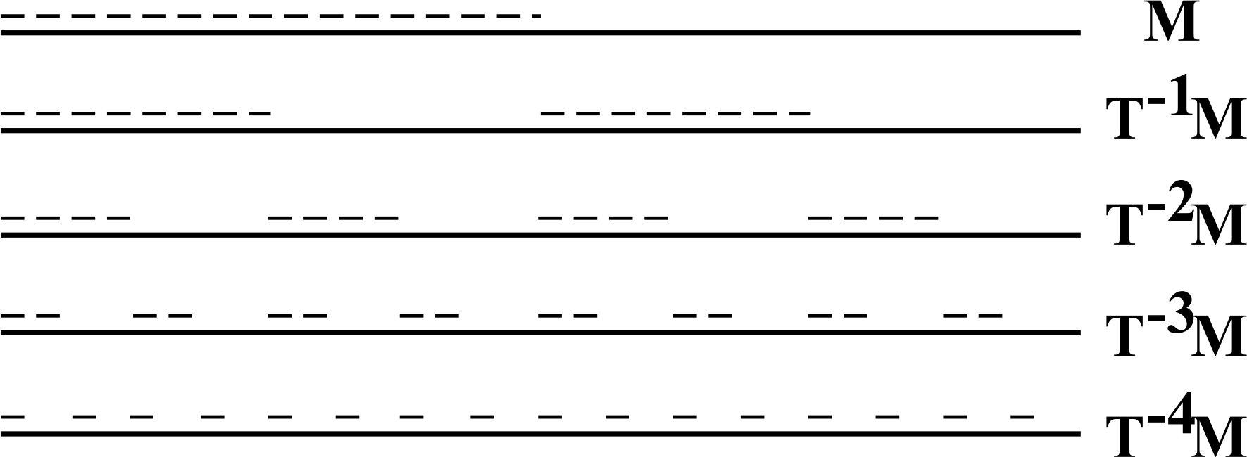
\begin{array}{l} | H (g, 𝒫_{n}^{E}) - H (g, 𝒫_{n}^{F}) | & \leq \sum_{i \in 𝒟_{s}} | g (μ (A_{i})) - g (μ (B_{i})) | + \frac{2}{s} d_{max} \\ \leq \sum_{i \in 𝒟_{s}} g (| μ (A_{i}) - μ (B_{i}) |) + \frac{2}{s} d_{max} \\ \leq \sum_{i \in 𝒟_{s}} g (μ (A_{i} Δ B_{i})) + \frac{2}{s} d_{max} \\ \leq \sum_{i = 1}^{m} g (μ (A_{i} Δ B_{i})) + \frac{2}{s} d_{max} \\ \leq 2^{n} g (δ) + \frac{2}{s} d_{max} \leq 1 + \frac{2}{s} d_{max} \end{array}

To find the lower bound for the g-entropy of a partition, we will use so-called independent sets. We construct the independent set in the following way: Let τ be a tower of height m. We divide the highest level of this tower (M_m₋₁) into two sets of equal measure, let us say I⁽^m⁻¹⁾ and M_m₋₁\I⁽^m⁻¹⁾. Next, we consider T⁻¹I⁽^m⁻¹⁾ and T⁻¹(M_m₋₁\I⁽^m⁻¹⁾). We divide each of them into two sets of equal measure, obtaining sets

I_{1}^{(m - 2)}, I_{2}^{(m - 2)}, I_{3}^{(m - 2)}, I_{4}^{(m - 2)}

, and define set I⁽^m⁻²⁾ as the algebraic sum of two of those sets—one subset of T⁻¹I⁽^m⁻¹⁾ and one of T⁻¹(M_m₋₁\I⁽^m⁻¹⁾). We perform this algorithm, until we achieve the lowest level of the tower — M₀ (see Figure 1). Eventually, we define

I : = \cup_{j = 0}^{m - 1} I^{(j)}

. We call this set an independent set in τ.

Figure 1. Set I (with dashes) in a tower a height of five.

We can make this construction, because every aperiodic system does not have atoms of positive measure, and in every non-atomic Lebesgue space for every measurable set A and every α ∈ [0, α], there exists B ⊂ A, such that μ(B) = α.

We are able to give an explicit formula for the g-entropy of the partition generated by the independent set in τ.

Lemma 7. Let τ = (M, TM,..., T²ⁿ⁻¹M) be the Rokhlin tower of height 2n and I ∈ Σ be an independent set in τ. If

g \in 𝒢_{0}^{\infty}

, then:

H_{τ_{0}^{n - 1}} (g, 𝒫_{n}^{I}) = \frac{μ (τ)}{2} φ (\frac{μ (τ)}{2^{n + 1}}),

where φ(x) = g(x)/x for x > 0.

Proof. The independence of I in τ implies that the partition:

𝒫_{n}^{I} \cap τ_{0}^{n - 1}

is a partition of

τ_{0}^{n - 1}

into 2ⁿ sets of equal measure 2⁻ⁿ

μ (τ_{0}^{n - 1})

. Therefore:

\begin{array}{l} H_{τ_{0}^{n - 1}} (g, 𝒫_{n}^{I}) & = \sum_{A \in 𝒫_{n}^{I}} g (μ (A \cap τ_{0}^{n - 1})) \\ = 2^{n} g (\frac{μ (τ_{0}^{n - 1})}{2^{n}}) = μ (τ_{0}^{n - 1}) φ (\frac{μ (τ_{0}^{n - 1})}{2^{n}}) \\ = \frac{μ (τ)}{2} φ (\frac{μ (τ)}{2^{n + 1}}) . \end{array}

Theorem 3. Let

g \in 𝒢_{0}^{\infty}

and T be an aperiodic, surjective automorphism of a Lebesgue space (X, Σ, μ), and let γ ∈ ℝ, then, there exists a partition

𝒫

∈ 𝔅, such that:

h (g, 𝒫) \geq γ .

Proof. We will prove that for any γ > 0, there exists a partition

𝒫

^E = {E, X\E}, such that h(g,

𝒫

) ≥ γ. We define recursively a sequence of sets E_n ∈ Σ. Let:

E_{0} : = \emptyset, N_{0} : = δ_{0} : = 1 .

Let n > 0, and assume that we have already defined E_n₋₁, N_n₋₁ and δ_n₋₁. Using Lemma 6, we can choose δ_n > 0, such that:

δ_{n} < \frac{1}{2} δ_{n - 1}

(7)

| H (g, 𝒫_{n}^{E_{n - 1}}) - H (g, 𝒫_{N_{n}}^{F}) | < 1 + \frac{2}{s} d_{max .}

(8)

for any F ∈ Σ, for which μ(E_n₋₁ ΔF) < 2δ_n.

Since:

lim_{x \to 0^{+}} \frac{g (x)}{η (x)} = \infty,

we can choose such N_n ∈ ℕ that:

\frac{φ (δ_{n} 2^{- N_{n} - 1})}{φ_{η} (δ_{n} 2^{- N_{n} - 1})} > \frac{2 γ}{δ_{n} log 2} .

(9)

By Lemma 4, there exists M_n ∈ Σ, such that τ_n = (M_n, TM_n,...,T^2N_n−1M_n) is a Rokhlin tower of measure μ(τ_n) = δ_n. Let I_n ⊂ τ_n be an independent set in τ_n and:

E_{n} : = (E_{n - 1} \ τ_{n}) \cup I_{n} .

Then:

μ (E_{n - 1} Δ E_{n}) \leq μ (τ_{n}) = δ_{n} .

for all positive integers n. By Equation (7), we have δ_n < 2⁻ⁿ, and we conclude that

{(1_{E_{n}})}_{n = 0}^{\infty}

is a Cauchy sequence in L₁(X). Therefore, there exist E ∈ Σ, such that 1_{E_n} converges to 1_E. For this set, we have:

μ (E_{n} Δ E) \leq \sum_{k = n + 1}^{\infty} μ (E_{k} Δ E_{k - 1}) \leq \sum_{k = n + 1}^{\infty} δ_{k} < 2 δ_{n + 1} .

Since E_n ∩ τ_n = I_n, applying Equation (8) and Lemmas 5 and 7, we obtain that for N_n, such that δ_n · 2^−N_n−1 < s:

\begin{array}{l} H (g, 𝒫_{N_{n}}^{E}) & \geq & H (g, 𝒫_{N_{n}}^{E_{n}}) - 1 - \frac{2}{s} d_{max} \\ \geq & H_{{(τ_{n})}_{0}^{N_{n} - 1}} (g, 𝒫_{N_{n}}^{E_{n}}) - (\frac{2}{s} + 3) d_{max} - 1 \\ \geq & H_{{(τ_{n})}_{0}^{N_{n} - 1}} (g, 𝒫_{N_{n}}^{I_{n}}) - (\frac{2}{s} + 3) d_{max} - 1 \\ \geq & [\frac{μ (τ_{n}) ln 2}{2}] (N_{n} + 1) - \frac{μ (τ_{n}) ln μ (τ_{n})}{2} . \frac{φ (μ (τ_{n}) 2^{- N_{n} - 1})}{- ln (μ (τ_{n}) 2^{- N_{n} - 1})} \\ - (\frac{2}{s} + 3) d_{max} - 1 \\ \geq & \frac{ln 2}{2} \cdot δ_{n} \cdot (N_{n} + 1) \cdot \frac{φ (δ_{n} 2^{- N_{n} - 1})}{φ_{η} (δ_{n} 2^{- N_{n} - 1})} - (\frac{2}{s} + 3) d_{max} - 1 . \end{array}

From Equation (9), we obtain that:

lim_{x \to \infty} \frac{H (g, 𝒫_{N_{n}}^{E})}{N_{n}} \geq \frac{ln 2}{2} lim_{n \to \infty} δ_{n} \cdot \frac{N_{n} + 1}{N_{n}} \cdot \frac{φ (δ_{n} 2^{- N_{n} - 1})}{φ_{η} (δ_{n} 2^{- N_{n} - 1})} \geq γ .

Thus,

\underset{n \to \infty}{lim sup} \frac{1}{n} H (g, 𝒫_{n}) \geq γ .

2.1.3. Bernoulli Shifts

Let 𝒜 = {1,...,k} be a finite alphabet. Let

X = {x = {x_{i}}_{i = - \infty}^{\infty} : x_{i} \in 𝒜}

and σ be a left shift:

σ {(x)}_{i} = x_{i + 1} .

For any s ≤ t and block [ω₀, ... ,ω_t₋_s] with a_i ∈𝒜, we define a cylinder:

C_{s}^{t} (ω_{0}, \dots, ω_{t - s}) = {x \in X : x_{i} = ω_{i - s} for i = s, \dots, t} .

We consider a Borel σ-algebra with respect to the metric, which is given by d(x, y) = 2^−N, where N = min{|i| : x_i ≠ y_i}. Let p = (p₁,..., p_k) be a probability vector. We define a measure ρ = ρ(p) on 𝒜 by setting ρ({i}) = p_i. Then, μ_p is a corresponding product measure on X = 𝒜^𝕑. Thus, the static g-entropy of a partition

𝒫

^𝒜 = {[1], [2],..., [k]} is equal to:

H_{μ_{p}} (g, 𝒫_{n}^{𝒜}) = \sum_{ω \in 𝒜^{n}} g (μ (C_{0}^{n - 1} (ω_{0}, \dots, ω_{n - 1}))) = \sum_{ω \in 𝒜^{n}} g (p_{ω_{0}} \dots p_{ω_{n - 1}}),

where ω = (ω₀,...,ω_n₋₁). By the concavity of g, we have:

H_{μ_{p}} (g, 𝒫_{n}^{𝒜}) \leq φ (1 / k^{n})

where equality holds only when

p = p^{*} = (\frac{1}{k}, \dots, \frac{1}{k})

. Before calculating the dynamical g-entropy of

𝒫

^𝒜 with respect to μ_p^*, we give the following lemma, the proof of which will be given later:

Lemma 8. If g ∈

𝒢

₀, then:

Cs (g) = \underset{n \to \infty}{lim sup} \frac{g (κ^{- n})}{η (κ^{- n})} and Ci (g) = \underset{n \to \infty}{lim inf} \frac{g (κ^{- n})}{η (κ^{- n})}

for any κ > 1.

Therefore, applying Lemma 8 for the partition

𝒫

^𝒜 and κ = k, we obtain:

h_{μ_{p^{*}}} (g, 𝒫^{𝒜}) = \underset{n \to \infty}{lim sup} \frac{1}{n} φ (\frac{1}{k^{n}}) = {\begin{array}{l} Cs (g) \cdot log k, & if Cs (g) < \infty; \\ \infty, & otherwise . \end{array}

(10)

Remark 2. If we consider the lower limit instead of the upper limit, we would obtain:

\underset{n \to \infty}{lim inf} \frac{1}{n} φ (\frac{1}{k^{n}}) = {\begin{array}{l} Ci (g) \cdot log k, & i f Ci (g) < \infty; \\ \infty, & otherwise . \end{array}

Therefore, we cannot replace an upper limit by the limit in the definition of the dynamical g-entropy.

Proof of Lemma 8. We will show just the equality for the upper limit, since the equality for the lower limit may be obtained analogously. Let

{(x_{n})}_{n = 1}^{\infty}

and

{(m_{n})}_{n = 1}^{\infty}

be such that

\underset{n \to \infty}{lim sup} g (x_{n}) / η (x_{n}) = c

and x_n ∈ (κ^−m_n,κ^−m_n+1) for every n ∈ ℕ. Then, –log x_n ≥ – log κ^−m_n+1. Every g ∈

𝒢

₀ is quasi-homogenic; so, for every positive integer n occurs:

\frac{g (x_{n})}{x_{n}} < \frac{g (κ^{- m_{n}})}{κ^{- m_{n}}} .

Therefore:

\begin{array}{l} \frac{g (x_{n})}{η (x_{n})} & = \frac{g (x_{n})}{x_{n}} \frac{1}{- log x_{n}} \leq \frac{g (κ^{- m_{n}})}{κ^{- m_{n}}} \frac{1}{(m_{n} - 1) log κ} \\ = \frac{g (κ^{- m_{n}})}{η (κ^{- m_{n}})} \cdot \frac{m_{n}}{m_{n} - 1}, \end{array}

and:

\underset{x \to 0^{+}}{lim sup} \frac{g (x)}{η (x)} = \underset{n \to \infty}{lim sup} \frac{g (κ^{- n})}{η (κ^{- n})} .

2.2. Kolmogorov-Sinai Entropy-Like Invariant

The basic tool considered in the ergodic theory is the Kolmogorov–Sinai entropy, which is a supremum of Shannon dynamical entropies over all finite partitions:

h_{μ} (T) = sup_{𝒫 \in 𝔅} h (T, 𝒫) .

It is invariant under metric isomorphism. Following the Kolmogorov proposition, we take the supremum over all partitions of the dynamical g-entropy of a partition. For a given system (X, Σ, μ, T), we define:

h_{μ} (g, T) = sup_{𝒫 \in 𝔅} h (g, T, 𝒫)

(11)

and call it the measure-theoretic g-entropy of transformation T with respect to measure μ.

It is easy to see that it is an isomorphism invariant. Ornstein and Weiss [23] showed the striking result that measure-theoretic entropy is the only finitely observable invariant for the class of all ergodic processes. More precisely, every finitely observable invariant for a class of all ergodic processes is a continuous function of entropy. Of course, in the case of

g \in 𝒢_{0}^{0} \cup 𝒢_{0}^{Sh}

by Corollary 2, we have:

h_{μ} (g, T) = lim_{x \to 0^{+}} \frac{g (x)}{η (x)} \cdot h_{μ} (T) .

We will show that for a wider class of functions, namely for those for which:

Cs (g) = \underset{x \to 0^{+}}{lim sup} \frac{g (x)}{η (x)} < \infty

we have:

h_{μ} (g, T) = Cs (g) \cdot h_{μ} (T)

for any ergodic transformation T. This shows that the measure-theoretic g-entropy is, in fact, finitely observable: one might simply compose the entropy estimators [25] with the linear function itself. Our proof will be similar to the proof of ([12], Theorem 1.1) where Takens and Verbitski showed that for ergodic transformations, the supremum over all finite partitions of dynamical Rényi entropies of order α > 1 are equal to the measure-theoretic entropy of T with respect to measure μ.

Let us introduce necessary definitions and facts. Let T_i be automorphisms of Lebesgue space (X_i, Σ_i, μ_i) for i = 1, 2, respectively. Then, we say that T₂ is a factor of transformation T₁, if there exists a homomorphism ϕ: X₁ ↦ X₂, such that:

ϕ T_{1} = T_{2} ϕ μ_{1} a . e . on X_{1} .

Suppose that T₂ is a factor of T₁ under homomorphism ϕ. Then, for an arbitrary finite partition

𝒫

of X₂, we have:

H (g, \lor_{i = 0}^{k - 1} T_{2}^{- i} 𝒫) = H (g, \lor_{i = 0}^{k - 1} ϕ^{- 1} T_{2}^{- i} 𝒫) = H (g, \lor_{i = 0}^{k - 1} T_{1}^{- i} ϕ^{- 1} 𝒫) .

Hence, h(g, T₂,

𝒫

) = h(g, T₁, ϕ⁻¹

𝒫

). Therefore:

h_{μ} (g, T_{2}) = sup_{𝒫 - finite} h (g, T_{2}, 𝒫) = sup_{𝒫 - finite} h (g, T_{1}, ϕ^{- 1} 𝒫) \leq h (g, T_{1}) .

This implies the following proposition:

Proposition 1. If T₂ is a factor of T₁, then for every function g ∈

𝒢

₀:

h_{μ} (g, T_{2}) \leq h_{μ} (g, T_{1}) .

2.2.1. Measure-Theoretic g-Entropies for Bernoulli Automorphisms

An automorphism T on (X, Σ, μ) is called Bernoulli automorphism if it is isomorphic to some Bernoulli shift. The crucial role in the proof of the main theorem of this section (Theorem 5) will be played by a well-known Sinai theorem:

Theorem 4 (Sinai [33]). Let T be an arbitrary ergodic automorphism of some Lebesgue space (X, Σ, μ). Then, each Bernoulli automorphism with h_μ(T₁) ≤ h_μ(T) is a factor of the automorphism T.

We start proving the following proposition:

Proposition 2. Let T be an arbitrary ergodic automorphism with h_μ(T) ≥ log M for some integer M ≥ 2. Then, for every g ∈

𝒢

₀:

h_{μ} (g, T) \geq Cs (g) \cdot log M .

Proof. Consider a shift σ over the alphabet 𝒜 = {0, 1 ..., M – 1} with the corresponding Bernoulli measure generated by

p_{1} = \dots = p_{M} = \frac{1}{M}

. It is easy to see that h_μ(σ) = log M. From Theorem 4, we conclude that σ is a factor of T . Therefore, applying formula (10), we obtain:

h_{μ} (g, T) \geq h_{μ} (g, σ) \geq h (g, σ, 𝒫^{𝒜}) = \underset{n \to \infty}{lim sup} \frac{1}{n} φ (M^{- n}) = log M \cdot \underset{n \to \infty}{lim sup} \frac{φ (M^{- n})}{φ_{η} (M^{- n})} .

Applying Lemma 8 completes the proof.

2.2.2. Main Theorem

Our goal in this section is the following result:

Theorem 5. Let T be an ergodic automorphism of Lebesgue space (X, Σ, μ), and g ∈

𝒢

₀ be such that Cs(g) ∈ (0, ∞). Then:

h_{μ} (g, T) = {\begin{array}{l} Cs (g) \cdot h_{μ} (T), & i f h_{μ} (T) < \infty, \\ \infty, & otherwise . \end{array}

If

g \in 𝒢_{0}^{0}

, then h_μ(g, T) = 0. If g ∈

𝒢

₀ is such that Cs(g) = ∞ and T has a positive measure-theoretic entropy, then h_μ(g, T) = ∞.

Moreover, for

g \in 𝒢_{0}^{\infty}

from Theorem 3, we have:

Corollary 5. Let

g \in 𝒢_{0}^{\infty}

. If (X, T) is aperiodic and surjective, then h_μ(g, T) = ∞.

To prove Theorem 5, we need the first few preliminary lemmas.

Lemma 9. If T is an automorphism of the Lebesgue space (X, Σ, μ), then for every g ∈

𝒢

₀:

h_{μ} = (g, T^{m}) \leq m h_{μ} (g, T) .

Proof. Let

𝒫

∈ 𝔅, m ∈ ℕ. We have:

\begin{array}{l} h (g, T, 𝒫) & = \underset{k \to \infty}{lim sup} \frac{1}{k} H (g, 𝒫 \lor T^{- m} 𝒫 \lor \dots \lor T^{- m (k - 1)} 𝒫) \\ = lim_{n \to \infty} sup_{k \geq n} \frac{1}{k} H (g, 𝒫 \lor T^{- m} 𝒫 \lor \dots \lor T^{- m (k - 1)} 𝒫) . \end{array}

Fix k ∈ ℕ. Then,

\lor_{i = 0}^{n - 1} T^{- i} 𝒫

is a refinement of

𝒫

∨ T⁻^m

𝒫

∨ ...∨ T⁻^m⁽^k⁻¹⁾

𝒫

for n = km,..., k(m+1) − 1.

Therefore:

\begin{array}{l} \frac{1}{k} H (g, 𝒫 \lor T^{- m} 𝒫 \lor \dots \lor T^{- m (k - 1)} 𝒫) & \leq \frac{1}{k} H (g, 𝒫_{n - 1}) = \frac{n}{k} \frac{1}{n} H (g, 𝒫_{n - 1}) \\ \leq \frac{k m + m - 1}{k} \frac{1}{n} H (g, 𝒫_{n - 1}) \\ \leq m (1 + \frac{1}{k}) \frac{1}{n} H (g, 𝒫_{n - 1}) \end{array}

(12)

for n = km,..., k(m +1) – 1. Let us introduce the following notation:

c_{k} : = \frac{1}{k} H (g, 𝒫 \lor T^{- m} 𝒫 \lor \dots \lor T^{- m (k - 1)} 𝒫), a_{n} : = \frac{1}{n} H (g, 𝒫_{n - 1}) .

Then, we can rewrite Equation (12) in the form:

c_{k} \leq m (1 + \frac{1}{k}) a_{n}

(13)

for n = km,..., km + m – 1. Taking the supremum in Equation (13), we obtain:

sup_{l \geq k} c_{l} \leq m (1 + \frac{1}{k}) sup_{n = l m, \dots, l (m + 1) - 1} a_{n} \leq m (1 + \frac{1}{k}) sup_{n \geq k m} a_{n} .

Therefore:

\underset{k \to \infty}{lim sup} c_{k} \leq m \underset{n \to \infty}{lim sup} a_{n},

and this is equivalent to the statement:

h (g, T^{m}, 𝒫) \leq m h (g, T, 𝒫) .

Taking the supremum over all finite partitions, we obtain the assertion.

Next, the lemma will be just a weaker version of Theorem 5.

Lemma 10. If an automorphism T^m of a Lebesgue space (X, Σ, μ) is ergodic for every m ∈ ℕ, then for every g ∈

𝒢

₀, such that Cs(g) < ∞ holds:

h_{μ} (g, T) \leq Cs (g) \cdot h_{μ} (T) .

If

g \in 𝒢_{0}^{0}

, then h_μ(g, T) = 0. If g ∈

𝒢

₀ is such that Cs(g) = ∞ and T has a positive Kolmogorov-Sinai entropy, then h_μ(g, T) = ∞.

Proof. The case of

g \in 𝒢_{0}^{0}

follows from Corollary 2. Suppose that there exists such

g \in 𝒢_{0} \ 𝒢_{0}^{0}

, which fulfills the assumptions of the lemma and for which we have:

Cs (g) \cdot h_{μ} (T) - h_{μ} (g, T) > 0 .

Then, applying Lemma 9 to the transformation T^m and using equality h_μ(T^m) = mh_μ(T) (see [2], Theorem 4.3.16), we obtain:

Cs (g) h_{μ} (T^{m}) - h_{μ} (g, T^{m}) \geq m (Cs (g) h_{μ} (T) - h_{μ} (g, T)) \to \infty as m \to \infty .

Therefore, for sufficiently large m, there exists an integer M for which:

h_{μ} (g, T^{m}) \leq m h_{μ} (g, T) < Cs (g) log M \leq m Cs (g) h_{μ} (T) = Cs (g) h_{μ} (T^{m}) .

(14)

Proposition 2 applied to the transformation T^m guarantees that for every g ∈

𝒢

₀ with positive (finite) Cs(g), we have:

h_{μ} (g, T^{m}) \geq Cs (g) log M .

(15)

Comparing Equations (14) and (15), we obtain the contradiction, which implies that

h_{μ} (g, T) = Cs (g) h_{μ} (T) .

If Cs(g) = ∞ and h_μ(T) > 0, then there exists such an integer m > 0 that:

h_{μ} (T^{m}) = m h_{μ} (T) > log M

and by Proposition 2 and Lemma 9:

h_{μ} (g, T) = h_{μ} (g, T^{m}) = \infty

which completes the proof.

Proof of Theorem 5. If h_μ(T) = 0, the statement is true, because for any

𝒫

∈ 𝔅, we have:

0 \leq h (g, 𝒫) \leq Cs (g) h (𝒫) = 0 .

Suppose that 0 < h_μ(T) < ∞. Automorphism T is ergodic. Thus, it has a factor, which is a Bernoulli automorphism T′ with h_μ(T) = h_μ(T′). Every Bernoulli automorphism is mixing, so T^m is ergodic for each m. Applying Lemma 10, we obtain:

h_{μ} (g, T^{'}) = Cs (g) h_{μ} (T^{'}) = Cs (g) h_{μ} (T) .

Since T′ is a factor of T, Proposition 1 implies that:

Cs (g) h_{μ} (T) = Cs (g) h_{μ} (T^{'}) = h_{μ} (g, T^{'}) \leq h_{μ} (g, T) \leq Cs (g) h_{μ} (T)

which completes the proof of the case of finite h_μ(T). If h_μ(T) = ∞, then Proposition 2 implies that:

h_{μ} (g, T) \geq Cs (g) log M

for every M > 0.

2.2.3. Generator Theorem Counterpart

In the case of

g \in 𝒢_{0}^{\infty}

, there is no counterpart of a Kolmogorov-Sinai generator theorem, which states that the measure-theoretic entropy of the transformation T is realized on every generator of the σ-algebra Σ. Let us consider Sturm shifts, shifts that model translations of the circle 𝕋 = [0, 1). Let β ∈ [0, 1) and consider the translation ϕ_β :[0, 1) ↦ [0, 1) defined by ϕ_β(x) = x + β (mod 1). Let

𝒫

denote the partition of [0, 1) given by

𝒫

= {[0,β), [β, 1)}. Then, we associate a binary sequence to each t ∈ [0, 1) according to its itinerary relative to

𝒫

; that is, we associate to t ∈ [0, 1) the bi-infinite sequence x defined by x_i =0 if

ϕ_{β}^{i}

(t) ∈ [0,β) and x_i =1 if

ϕ_{β}^{i}

(t) ∈ [β, 1). The set of such sequences is not necessary closed, but it is shift-invariant and so its closure is a shift space called the Sturmian shift. If β is irrational, then Sturmian shift is minimal, i.e., there is no proper subshift. Moreover, for a minimal Sturmian shift, the number of n-blocks that occur in an infinite shift space is exactly n +1. Therefore for zero-coordinate partition

𝒫

^𝒜, which is a finite generator of σ-algebra Σ, and for any function g ∈

𝒢

₀, we have:

H (g, 𝒫_{n}^{𝒜}) = \sum_{A \in 𝒫_{n}^{𝒜}} g (μ_{S} (A)) \leq φ (\frac{1}{n + 1})

where μ_S is the unique invariant measure for Sturm shift. Thus,

h (g, 𝒫^{𝒜}) \leq \underset{n \to \infty}{lim sup} \frac{n + 1}{n} g (\frac{1}{n + 1}) = 0 .

On the other hand, since it is strictly ergodic (thus aperiodic), Theorem 3 implies that for any

g \in 𝒢_{0}^{\infty}

:

h_{μ} (g, T) = \infty .

Therefore, we have a finite generator, for which the supremum is not attained.

3. Discussion

In this note, we discussed the generalization of the dynamical and Kolmogorov-Sinai entropy based on the idea of considering in the definition of the dynamical entropy a concave function vanishing at the origin instead of the Shannon entropy function η. The connections between dynamical entropies and g-entropies show that the crucial property of η for applications of the Shannon entropy in the dynamical systems is the behavior of η in the neighborhood of zero. Additionally, the main result of the paper obtained for the generalization of the KS entropy states that, usually, there is a linear dependence between the obtained invariant and the KS entropy. It also implies (due to the fact that it is a continuous function of the entropy) that the measure-theoretic g-entropy is finitely observable (see, e.g., [23]). Moreover, considering functions that behave in the neighborhood of zero differently than the Shannon function usually trivializes the theory. On the other hand, we showed that if the limit of g/η at zero is infinite, then for every positive number γ, there exists a partition for which the g-entropy will be greater than or equal to γ. Thus, the measure-theoretic g-entropy will be infinite. The example from Section 2.2.3, based on this result, implies that there is no counterpart of the generator theorem (e.g., Tsallis entropies for α< 1, which we obtain considering

g (x) = \frac{x = x^{α}}{α - 1}

with α ∈ (0, 1), fit into this scheme). However, the concept of g-entropies is still of use, e.g., considering the rate of convergence of partial g-entropies may give additional information about the system [30]. The most promising direction in this context seems to be considering functions for which C(g) = 0 and g′(0) = ∞.

Conflicts of Interest

The author declares no conflict of interest.

References

Downarowicz, T. Entropy in Dynamical Systems; Cambridge University Press: New York, NY, USA, 2011. [Google Scholar]
Katok, A.; Hasselblatt, B. Introduction to the Modern Theory of Dynamical Systems; Cambridge University Press: New York, NY, USA, 1997. [Google Scholar]
Misiurewicz, M. A short proof of the variational principle for 𝕑ⁿ₊ action on a compact space. Astérisque 1976, 40, 147–157. [Google Scholar]
Shannon, C.E. A mathematical theory of communication. Bell Syst. Tech. J 1948, 27. [Google Scholar]
Rényi, A. On measures of entropy and information. In Proceedings of the 4th Berkeley Symposium on Mathematical Statistics and Probability, 20 June–30 July 1960; University of California Press: Berkeley, CA, USA, 1961; Volume 1. Statistical Laboratory of the University of California: Berkeley, CA, USA; pp. 547–561.
Arimoto, S. Information-theoretical considerations on estimation problems. Inf. Control 1971, 19, 181–194. [Google Scholar]
Wu, Y.; Verdú, S. Rényi Information Dimension: Fundamental Limits of Almost Lossless Analog Compression. IEEE Trans. Inf. Theory 2010, 56, 3721–3748. [Google Scholar]
Csiszár, I. Axiomatic characterization of information measures. Entropy 2008, 10, 261–273. [Google Scholar]
De Paly, T. On entropy-like invariants for dynamical systems. Z. Anal. Anwend 1982, 1, 69–79. [Google Scholar]
De Paly, T. On a class of generalized K-entropies and Bernoulli shifts. Z. Anal. Anwend 1982, 1, 87–96. [Google Scholar]
Grassberger, P.; Procaccia, I. Estimation of the Kolmogorov entropy from a chaotic signal. Phys. Rev. A 1983, 28, 2591–2593. [Google Scholar]
Takens, F.; Verbitski, E. Generalized entropies: Rényi and correlation integral approach. Nonlinearity 1998, 11, 771–782. [Google Scholar]
Takens, F.; Verbitski, E. Rényi entropies of aperiodic dynamical systems. Isr. J. Math 2002, 127, 279–302. [Google Scholar]
Liu, Q.; Cao, K.-F.; Peng, S.-L. A generalized Kolmogorov–Sinai-like entropy under Markov shifts in symbolic dynamics. Physica A 2009, 388, 4333–4344. [Google Scholar]
Mesón, A.M.; Vericat, F. Invariant of dynamical systems: A generalized entropy. J. Math. Phys 1996, 37, 4480–4483. [Google Scholar]
Mesón, A.M.; Vericat, F. On the Kolmogorov-like generalization of Tsallis entropy, correlation entropies and multifractal analysis. J. Math. Phys 2002, 43, 904–918. [Google Scholar]
Havrda, J.; Charvàt, F. Quantification method of classification processes. Concept of structural α-entropy. Kybernetika 1967, 3, 30–35. [Google Scholar]
Abe, S. Tsallis entropy: How unique? Contin. Mech. Thermodyn 2004, 16, 237–244. [Google Scholar]
Furuichi, S. Information theoretical properties of Tsallis entropies. J. Math. Phys 2006, 47, 023302. [Google Scholar]
Tsallis, C. Possible generalization of Boltzmann–Gibbs statistics. J. Stat. Phys 1988, 52, 479–487. [Google Scholar]
Tsallis, C. Entropic nonextensivity: A possible measure of complexity. Chaos Solitons Fractals 2002, 13, 371–391. [Google Scholar]
Tsallis, C.; Plastino, A.R.; Zheng, W.-M. Power-law sensitivity to initial conditions—New entropic representation. Chaos Solitons Fractals 1997, 8, 885–891. [Google Scholar]
Ornstein, D.S.; Weiss, B. Entropy is the only finitely observable invariant. J. Mod. Dyn 2007, 1, 93–105. [Google Scholar]
Weiss, B. (The Hebrew University of Jerusalem); 2013; personal communication.
Weiss, B. Single Orbit Dynamics; American Mathematical Society: Providence, RI, USA, 2000. [Google Scholar]
Blume, F. The Rate of Entropy Convergence, University of North Carolina, Chapel Hill, NC, USA, 1995.
Blume, F. Possible rates of entropy convergence. Ergod. Theory Dyn. Syst 1997, 17, 45–70. [Google Scholar]
Galatolo, S. Global and local complexity in weakly chaotic dynamical systems. Discret. Contin. Dyn. Syst 2003, 9, 1607–1624. [Google Scholar]
Ferenczi, S.; Park, K.K. Entropy dimensions and a class of constructive examples. Discret. Contin. Dyn. Syst 2007, 17, 133–141. [Google Scholar]
Falniowski, F. Possible g-entropy convergence rates. 2013, arXiv. 1309.6246. [Google Scholar]
Rosenbaum, R.A. Sub-additive functions. Duke Math. J 1950, 17, 227–247. [Google Scholar]
Heinemann, S.-M.; Schmitt, O. Rokhlin’s Lemma for non-invertible maps. Dyn. Syst. Appl 2001, 10, 201–214. [Google Scholar]
Sinai, Y.G. Weak isomorphism of transformation with an invariant measure. Sov. Math 1962, 3, 1725–1729. [Google Scholar]

© 2014 by the authors; licensee MDPI, Basel, Switzerland This article is an open access article distributed under the terms and conditions of the Creative Commons Attribution license (http://creativecommons.org/licenses/by/3.0/).

On the Connections of Generalized Entropies With Shannon and Kolmogorov–Sinai Entropies

Abstract

1. Introduction

2. Results

2.1. Basic Facts and Definitions

2.1.1. Dynamical g-Entropies

2.1.2. Case of $g \in 𝒢_{0}^{\infty}$

2.1.3. Bernoulli Shifts

2.2. Kolmogorov-Sinai Entropy-Like Invariant

2.2.1. Measure-Theoretic g-Entropies for Bernoulli Automorphisms

2.2.2. Main Theorem

2.2.3. Generator Theorem Counterpart

3. Discussion

Conflicts of Interest

References

Article Metrics

Citations

Article Access Statistics

On the Connections of Generalized Entropies With Shannon and Kolmogorov–Sinai Entropies

Abstract

1. Introduction

2. Results

2.1. Basic Facts and Definitions

2.1.1. Dynamical g-Entropies

2.1.2. Case of g ∈ 𝒢 0 ∞

2.1.3. Bernoulli Shifts

2.2. Kolmogorov-Sinai Entropy-Like Invariant

2.2.1. Measure-Theoretic g-Entropies for Bernoulli Automorphisms

2.2.2. Main Theorem

2.2.3. Generator Theorem Counterpart

3. Discussion

Conflicts of Interest

References

Article Metrics

Citations

Article Access Statistics

2.1.2. Case of $g \in 𝒢_{0}^{\infty}$