Bias Adjustment for a Nonparametric Entropy Estimator

Abstract

Zhang in 2012 introduced a nonparametric estimator of Shannon’s entropy, whose bias decays exponentially fast when the alphabet is finite. We propose a methodology to estimate the bias of this estimator. We then use it to construct a new estimator of entropy. Simulation results suggest that this bias adjusted estimator has a significantly lower bias than many other commonly used estimators. We consider both the case when the alphabet is finite and when it is countably infinite.

1. Introduction

Let $\mathcal{K}$ be a finite or countable index set with cardinality $\left|\mathcal{K}\right|$. Let $P=\{p_k:k\in \mathcal{K}\}$ be a probability distribution on the alphabet $\mathcal{X}=\{{\ell }_k;k\in \mathcal{K}\}$. Entropy, of the form

$$H=-\sum _{k\in \mathcal{K}}{p}_{k}ln\left(p_k\right)$$

(1)

was introduced by Shannon in [1] and is often referred to as Shannon’s entropy. Miller [2] and Basharin [3] were among the first to study nonparametric estimation of H. Since then, the topic has been investigated from a variety of directions and perspectives. Many important references can be found in [4] and [5]. In this paper, we introduce a modification of an estimator of entropy, which was first defined by Zhang in [6]. This modification aims to reduce the bias of the original estimator. Simulations suggest that, at least for the models considered, this estimator has very low bias compared with several other commonly used estimators. Throughout this paper, we use ln to denote the natural logarithm and we define, as is common, $0ln0=0$. For any two functions f and g, taking values in $(0,\infty )$ with $\underset{n\to \infty }{lim}f\left(n\right)=\underset{n\to \infty }{lim}g\left(n\right)=0$, we write $f\left(n\right)=\mathcal{O}\left(g\right(n\left)\right)$ to mean

$$\begin{array}{c}\hfill 0<\underset{n\to \infty }{lim\; inf}\frac{f\left(n\right)}{g\left(n\right)}\le \underset{n\to \infty }{lim\; sup}\frac{f\left(n\right)}{g\left(n\right)}<\infty \end{array}$$

and $\mathcal{O}\left(g\right(n\left)\right)\le f\left(n\right)$ to mean

$$\begin{array}{c}\hfill 0<\underset{n\to \infty }{lim\; inf}\frac{f\left(n\right)}{g\left(n\right)}\le \underset{n\to \infty }{lim\; sup}\frac{f\left(n\right)}{g\left(n\right)}\le \infty \end{array}$$

Assume that P is unknown. Let $X_1,X_2,\cdots ,X_n$ be an independent and identically distributed ($iid$) sample of size n from $\mathcal{X}$ according to P. Let $\left\{y_k={\sum }_{i=1}^{n}1[X_i={\ell }_k],k\in \mathcal{K}\right\}$ be the observed sample frequencies of letters in the alphabet, and let $\left\{{\widehat{p}}_k=y_k/n,k\in \mathcal{K}\right\}$ be the sample proportions. In this framework, we are interested in estimating H. Perhaps the most intuitive nonparametric estimator of H is given by

$$\begin{array}{c}\hfill \widehat{H}=-\sum _{k\in \mathcal{K}}{\widehat{p}}_{k}ln\left({\widehat{p}}_k\right)\end{array}$$

(2)

This is known as the plug-in estimator. When $\left|\mathcal{K}\right|$ is finite, the bias of $\widehat{H}$ is given by

$$\frac{\left|\mathcal{K}\right|-1}{2n}+\mathcal{O}(1/n^2)$$

see Miller [2] or, for a more formal treatment, Paninski [5]. This leads to the so-called Miller–Madow estimator

$$\begin{array}{c}\hfill {\widehat{H}}_{MM}=\widehat{H}+\frac{\widehat{\left|\mathcal{K}\right|}-1}{2n}\end{array}$$

(3)

where $\widehat{\left|\mathcal{K}\right|}$ is the number of distinct letters observed in the sample. Other estimators of H include the jackknife estimator of Zahl [7] and Strong, Koberle, de Ruyter van Steveninck, and Bialek [8], and the NSB estimator of Nemenman, Shafee, and Bialek [9] and Nemenman [10]. These estimators (and others) have been shown to work well in numerical studies, although many of their theoretical properties (such as consistency and asymptotic normality) are not known.

Zhang [6] proposed an estimator, ${\widehat{H}}_z$, of entropy, which is given in Equation (4) below. When $\left|\mathcal{K}\right|$ is finite, the bias of ${\widehat{H}}_z$ decays exponentially fast, and the estimator is asymptotically normal and efficient. See Zhang [11] for details. This estimator is given by

$${\widehat{H}}_z=\sum _{v=1}^{n-1}\frac{1}{v}{Z}_{1,v}$$

(4)

where

$$Z_{1,v}=\frac{n^{v+1}[n-(v+1)]!}{n!}\sum _{k\in \mathcal{K}}\left[{\widehat{p}}_k\prod _{j=0}^{v-1}\left(1-{\widehat{p}}_k-\frac{j}{n}\right)\right]$$

(5)

In Zhang [6] it is shown that

$$E({\widehat{H}}_z)=\sum _{v=1}^{n-1}\frac{1}{v}\sum _{k\in \mathcal{K}}{p}_k{(1-p_k)}^v$$

and that the bias of ${\widehat{H}}_z$ is given by

$$B_n=H-E({\widehat{H}}_z)=\sum _{v=n}^{\infty }\frac{1}{v}\sum _{k\in \mathcal{K}}{p}_k{(1-p_k)}^v$$

(6)

Although $B_n$ decays exponentially in n when $\mathcal{K}$ is a finite set, it can still be annoyingly sizable for small n. The objective of this paper is to put forth a good estimator ${\widehat{B}}_n$ of $B_n$, and, in turn, a good estimator of H by means of ${\widehat{H}}_z^{♯}={\widehat{H}}_z+{\widehat{B}}_n$. We deal with both the case when $\left|\mathcal{K}\right|$ is finite and the case when it is infinite.

2. Bias Adjustment

For a positive integer v, let ${\Delta }_v$ be the difference between the bias of ${\widehat{H}}_z$ based on an $iid$ sample of size v and that of size $v+1$, i.e.,

$${\Delta }_v=B_v-B_{v+1}=\frac{1}{v}\sum _{k\in \mathcal{K}}{p}_k{(1-p_k)}^v$$

Clearly $B_n={\sum }_{v=n}^{\infty }{\Delta }_v$. According to Zhang and Zhou [12], for every v with $1\le v\le n-1$, $Z_{1,v}$, as given in Equation (5), is the uniformly minimum variance unbiased estimator ($umvue$) of ${\zeta }_{1,v}={\sum }_{k\in \mathcal{K}}{p}_k{(1-p_k)}^v$. This implies that for every v, $1\le v\le n-1$, ${\widehat{\Delta }}_v=v^{-1}{Z}_{1,v}$ is a good estimator of ${\Delta }_v$.

The methodology proposed in this paper is as follows: For all $v\le n-1$, we estimate ${\Delta }_v$ with ${\widehat{\Delta }}_v$. We use ${\widehat{\Delta }}_1,{\widehat{\Delta }}_2,\cdots ,{\widehat{\Delta }}_{n-1}$ to fit a parametric function $\delta \left(v\right)$ such that $\delta \left(v\right)$ is close to ${\widehat{\Delta }}_v$. We then extrapolate this function and take ${\widehat{\Delta }}_v=\delta \left(v\right)$ for $v\ge n$. Our estimate of the bias is then ${\widehat{B}}_n={\sum }_{v=n}^{\infty }{\widehat{\Delta }}_n$.

It remains to choose a reasonable parametric form for δ and to fit it. We consider these questions in two separate cases: (1) when $\left|\mathcal{K}\right|$ is finite, known or unknown, and (2) when $\left|\mathcal{K}\right|$ is countably infinite. The case when it is unknown whether $\left|\mathcal{K}\right|$ is finite or infinite is discussed in Remark 1 below. Figure 1 shows how well our chosen $\delta \left(v\right)$ fits ${\widehat{\Delta }}_v$ for typical examples.

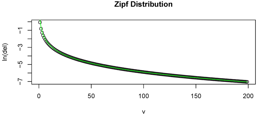
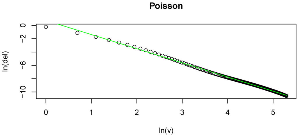
Figure 1. (a) Plot of v on the x-axis and $ln({\widehat{\Delta }}_v)$ on the y-axis. This is based on a random sample of size 200 from a Zipf distribution. The overlaid line is the estimated $ln\delta \left(v\right)$; (b) Plot of $ln\left(v\right)$ on the x-axis and $ln({\widehat{\Delta }}_v)$ on the y-axis. This is based on a random sample of size 200 from a Poisson distribution. The overlaid line is the estimated $ln\delta \left(v\right)$.

2.1. Case: $\left|\mathcal{K}\right|$ is Finite

Assume that $\left|\mathcal{K}\right|$ is finite. If $p_{\wedge }={min}_{k\in \mathcal{K}}{p}_k$ then

$${\Delta }_v=\frac{1}{v}\sum _{k\in \mathcal{K}}{p}_k{\left(1-p_k\right)}^v=\mathcal{O}\left(v^{-1}{\left(1-p_{\wedge }\right)}^v\right)$$

(7)

as v increases indefinitely. This suggests taking

$$\delta \left(v\right)=\frac{\alpha e^{-\gamma v}}{v}$$

(8)

where $\alpha >0$ and $\gamma >0$. However, since, for small values of v, other terms of the sum given in Equation (7) may have a significant impact, we consider the slightly more general form

$$\delta \left(v\right)=\frac{\alpha e^{-\gamma v}}{v^{\beta }}$$

(9)

where $\alpha >0$, $\gamma >0$ and $\beta \in \mathbb{R}$ are parameters. These parameters are estimated by using least squares to fit

$$ln{\delta }_v=ln\alpha -\beta lnv-\gamma v$$

(10)

with data

(11)

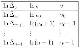
Here $v_0$ is a user-chosen positive integer. We can always take $v_0=1$, but we may wish to exclude the first several ${\widehat{\Delta }}_v$ since they may be atypical. We denote our estimate of $ln\alpha$ by $\widehat{ln\alpha }$, and those of α, β, and γ by

$$\widehat{\alpha }=e^{\widehat{ln\alpha }},\widehat{\beta },\mathrm{and}\widehat{\gamma }$$

(12)

The bias adjusted ${\widehat{H}}_z$ is given by

$${\widehat{H}}_z^{♯}={\widehat{H}}_z+\sum _{v=n}^{\infty }\left(\frac{\widehat{\alpha }{e}^{-\widehat{\gamma }v}}{v^{\widehat{\beta }}}\right)$$

(13)

This summation may be approximated by the integral ${\int }_n^{\infty }(\widehat{\alpha }{e}^{-\widehat{\gamma }v}{v}^{-\widehat{\beta }})\mathrm{d}v$ or by truncating the sum at some very large integer V. For the simulation results presented below, we take $v_0=10$ and $V=100,000$.

Two finer modifications are made to ${\widehat{H}}_z^{♯}$ in Equation (13) when the sample data present some undesirable features:

• If the least squares fit based on Equation (10) leads to $\widehat{\gamma }\le 0$, the fitted results are abandoned, and instead the new model

  $$ln{\delta }_v=ln\alpha -\gamma v$$

  (14)

  is fit to the same data as in Equation (11). The resulting estimates of the parameters are then

  $$\widehat{\alpha }=e^{\widehat{ln\alpha }}\mathrm{and}\widehat{\gamma }$$

  and a modified estimate of H is given by

  $${\widehat{H}}_z^{♯}={\widehat{H}}_z+\sum _{v=n}^{\infty }(\widehat{\alpha }{e}^{-\widehat{\gamma }v})$$

  (15)

  The switch from Equation (10) to Equation (14) is necessary because if $\widehat{\gamma }\le 0$ then ${\widehat{H}}_z^{♯}$ in Equation (13) diverges. In this case, we recommend taking a relatively large value for $v_0$ because small values of v are more likely to require a polynomial part. For our simulations, we use $v_0=(n-21)$ in this case.
• When a sample has no letters with frequency 1, the model in Equation (9) will not fit well. In this case we modify the sample by isolating one observation in a letter group with the least frequency and turn it into a singleton, e.g., a sample of the form $\{y_1,y_2,y_3\}=\{3,2,2\}$ is replaced by $\{3,2,1,1\}$.

To show how well Equation (9) fits $({\widehat{\Delta }}_1,{\widehat{\Delta }}_2,\cdots ,{\widehat{\Delta }}_{n-1})$ for a typical sample, we include an example of the fit in (a) of Figure 1. Here we plot v against $ln{\widehat{\Delta }}_v$. The overlaid curve represents the fitted $\delta \left(v\right)$. This is based on a simulation of a random sample of size 200 from a Zipf distribution. To give a snapshot of the performance of the proposed estimator, we conducted several numerical simulations, and compared the absolute value of the bias of the proposed estimator to that of several commonly used ones. The distributions that we performed the simulations on are:

• (Triangular) $p_k=k/5050$, for $k=1,2,\cdots ,100$, here $H\approx 4.416898$,
• (Zipf) $p_k=C/k$, for $k=1,2,\cdots ,100$, here $C\approx 0.192776$ and $H\approx 3.680778$.

The estimators that we compared the performance of our estimator to are: the plug-in estimator given in Equation (2), the Miller–Madow estimator given in Equation (3), and ${\widehat{H}}_z$ given in Equation (4).

For each distribution and each estimator, the bias was approximated as follows. We simulate n observations from the given distribution and evaluate the estimator. We then subtract the estimated value from the true value H. We repeat this 2000 times and average the errors. We then take the absolute value of the estimated bias. The procedure was slightly different for the estimator given in Equation (4). Since, in this case, the bias has the explicit form given in Equation (6), we approximate the bias by truncating this series at $100,000$. The sample sizes considered in these simulations range from $n=22$ to $n=500$. The plots of the estimated biases are graphed in Figure 2; part (a) gives the plot for the triangular distribution and part (b) gives the plot for the Zipf distribution. Note that our proposed estimator has the lowest bias in all cases and that it is significantly lower for small samples.

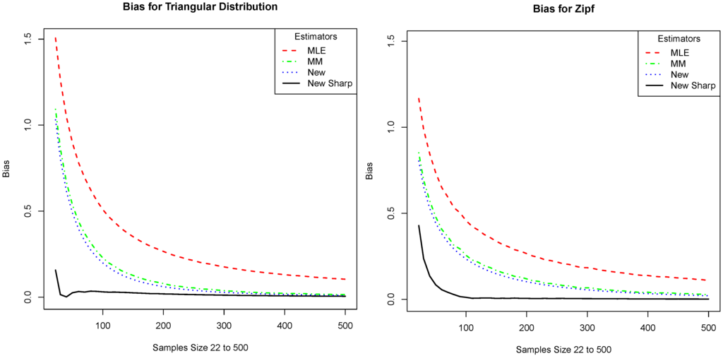
Figure 2. We compare the absolute value of the bias of our estimator (New Sharp) with that of the plug-in (MLE), the Miller–Madow (MM), and the one given in Equation (4) (New). The x-axis is the sample size and the y-axis is the absolute value of the bias. The plots correspond to the distributions: (a) Triangular distribution and (b) Zipf distribution.

Another estimator of entropy is the NSB estimator of Nemenman, Shafee, and Bialek [9] (see also Nemenman [10] and the references therein). The authors of that paper provide code to do the estimation, which is available at http://nsb-entropy.sourceforge.net/. We used version 1.13, which was updated on 20 July 2011. Unlike the estimators discussed above, this one requires knowledge of $\left|\mathcal{K}\right|$, and, for this reason, we consider it separately. Plots comparing the bias of our estimator and that of NSB are given in Figure 3. Note that our estimator is mostly comparable with NSB, although in certain regions it performs a bit better.

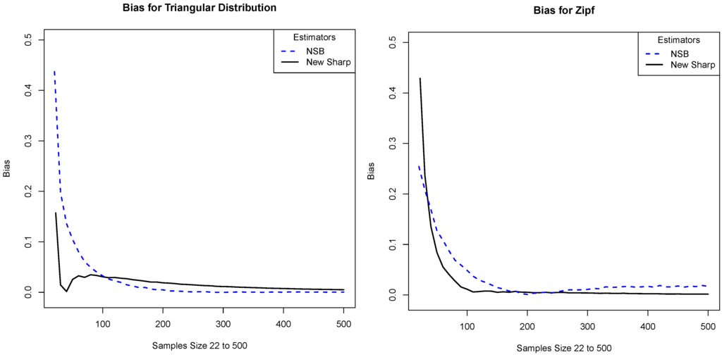
Figure 3. We compare the absolute value of the bias of our estimator with that of the NSB estimator. The x-axis is the sample size and the y-axis is the absolute value of the bias. The plots correspond to the distributions: (a) Triangular distribution and (b) Zipf distribution.

2.2. Case: $\left|\mathcal{K}\right|$ is Countably Infinite

We now turn to the case when $\left|\mathcal{K}\right|$ is countably infinite. We need to find a reasonable parametric form for $\delta \left(v\right)$. The following facts suggest an approach.

• For any distribution on a countably infinite alphabet ${\Delta }_v\ge \mathcal{O}\left(v^{-2}\right)$.
• If $p_k=C{k}^{-\lambda }$ for $k\ge 1$ where $\lambda >1$, then ${\Delta }_v=\mathcal{O}\left(v^{-(2-1/\lambda )}\right)$.

These facts tell us that ${\Delta }_v$ decays slower than $\mathcal{O}(1/v^2)$. Moreover, the heavier the tail of the distribution, the slower the decay appears to be. Since, even for very heavy tailed distributions, we have polynomial decay, this suggests that the rate of decay is essentially $\mathcal{O}(1/v^{\beta })$ for some $\beta \in (0,2]$. Thus, for all practical purposes, a reasonable model is

$$\delta \left(v\right)=\frac{\alpha }{v^{\beta }}$$

(16)

where $\alpha >0$ and $\beta >0$ (we allow $\beta >2$ to make the model more flexible). The model parameters are estimated by using least squares to fit

$$ln\delta \left(v\right)=ln\alpha -\beta lnv$$

(17)

with the data in Equation (11). We denote the estimate of $ln\alpha$ by $\widehat{ln\alpha }$, and those of α and β by

$$\widehat{\alpha }=e^{\widehat{ln\alpha }}\mathrm{and}\widehat{\beta }$$

(18)

The bias adjusted ${\widehat{H}}_z$ is given by

$${\widehat{H}}_z^{♯}={\widehat{H}}_z+\sum _{v=n}^{\infty }\left(\widehat{\alpha }{v}^{-\widehat{\beta }}\right)$$

(19)

where the summation may be approximated by the integral ${\int }_n^{\infty }(\widehat{\alpha }{v}^{-\widehat{\beta }})\mathrm{d}v=\widehat{\alpha }{n}^{1-\widehat{\beta }}/(1-\widehat{\beta })$ or by truncating the sum at some very large integer V. For the simulation results presented below, we take $v_0=10$ and use the integral approximation to the sum.

As in the case when $\left|\mathcal{K}\right|$ is finite, we need to make adjustments in certain situations.

• If $\widehat{\beta }\le 1$ then the sum in Equation (19) diverges. In fact, when $\widehat{\beta }$ is close to 1 (even if it is larger then 1), this causes problems. To deal with this we do the following. Choose ${\beta }_0\in (1,2]$, if $\widehat{\beta }<{\beta }_0$ our fitted results are abandoned, and instead the new model

  $$ln\delta \left(v\right)+{\beta }_{0}lnv=ln\alpha$$

  (20)

  is fit using least squares. In our simulations we take ${\beta }_0=1.5$. The resulting estimate of the sole parameter α is given by $\widehat{\alpha }=e^{\widehat{ln\alpha }}$, and a modified estimate of H is given by

  $${\widehat{H}}_z^{♯}={\widehat{H}}_z+\sum _{v=n}^{\infty }\left(\widehat{\alpha }{v}^{-{\beta }_0}\right)$$

  (21)
• When a sample has no letters with frequency 1, we run into trouble as we did in the case when $\left|\mathcal{K}\right|$ is finite. We solve this problem in the same way as in the previous case.

To show how well Equation (16) fits $({\widehat{\Delta }}_1,{\widehat{\Delta }}_2,\cdots ,{\widehat{\Delta }}_{n-1})$ in a typical sample, we include an example of the fit in (b) of Figure 1. Here we plot $lnv$ against $ln{\widehat{\Delta }}_v$. The overlaid curve represents the fitted $\delta \left(v\right)$. This is based on a simulation of a random sample of size 200 from a Poisson distribution. As in the previous case, we evaluate the performance of the proposed estimator by conducting several numerical simulations. We estimated entropy for the following distributions:

• (Power) $p_k=C/k^2$, for $k\ge 1$, here $C=6/{\pi }^2$ and $H\approx 1.637622$,
• (Geometric) $p_k=(1-1/e)e^{-k}$, for $k\ge 0$, here $H\approx 1.040652$,
• (Poisson) $p_k=e^{-\lambda }{\lambda }^k/k!$, for $k\ge 0$, where $\lambda =e$ and $H\approx 1.87722$.

Again, we compare with the plug-in estimator, the Miller–Madow estimator, and ${\widehat{H}}_z$. Although the Miller–Madow estimator is motivated by the case where $\left|\mathcal{K}\right|$ is finite, it is often a good estimator in the infinite case as well. We approximate the bias, as in the previous case. The estimated biases for sample sizes ranging from $n=22$ to $n=500$ are graphed in Figure 4. Parts (a), (b), and (c) of Figure 4 correspond to the three distributions listed above. Note that the new estimator outperforms the other estimators. However, the improvement is not as drastic as in the case when $\left|\mathcal{K}\right|$ is finite. We also make separate comparisons with NSB. These are given in Figure 5. Although NSB is designed for the case when $\left|\mathcal{K}\right|$ is known and finite, we can extend its use to the infinite case by telling the program that $\left|\mathcal{K}\right|$ is some large but finite value. In our simulations we take it to be ${10}^{10}$. We see that the performance of our estimator is roughly comparable with or somewhat better than that of NSB.

Remark 1.

In practice, it may not be known, a priori, if $\left|\mathcal{K}\right|$ is finite or infinite. In such situations, one does not know which of the two adjustments to use. One approach is as follows. Fit both models and denote their respective mean squared errors by $MS{E}_1$ and $MS{E}_2$, then use the one that has the smaller $MSE$.

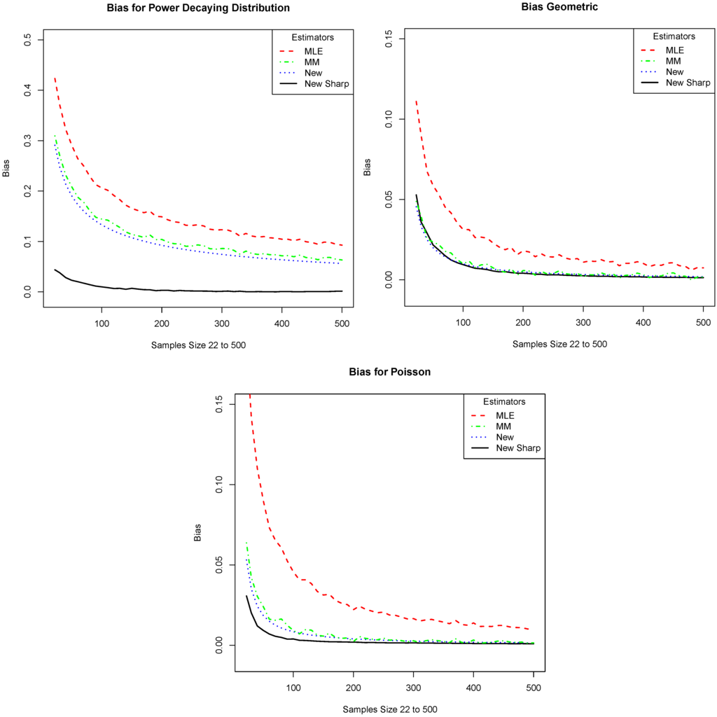
Figure 4. We compare the absolute value of the bias of our estimator (New Sharp) with that of the plug-in (MLE), the Miller–Madow (MM), and the one given in Equation (4) (New). The x-axis is the sample size and the y-axis is the absolute value of the bias. The plots correspond to the distributions: (a) Power; (b) Geometric; and (c) Poisson.

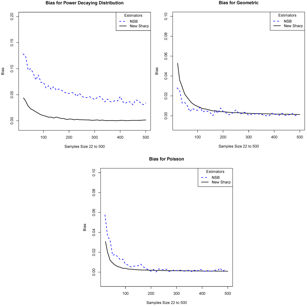
Figure 5. We compare the absolute value of the bias of our estimator with that of the NSB estimator. The x-axis is the sample size and the y-axis is the absolute value of the bias. The plots correspond to the distributions: (a) Power; (b) Geometric; and (c) Poisson.

3. Summary and Discussion

In Zhang [6] an estimator of entropy was introduced, which, in the case of a finite alphabet, has exponentially decaying bias. In this paper we described a methodology for further reducing the bias of this estimator. Our approach is to note that when the alphabet is finite, the bias of this estimator decays exponentially fast, while in the case when the alphabet is infinite, the bias decays like a polynomial. We estimate the bias by fitting an appropriate function. Then we add this estimate of the bias to our estimated entropy. Simulation results suggest that, at least in the situations considered, the bias is drastically reduced for small sample sizes. Moreover, our estimator outperforms several standard estimators and is comparable with the well-known estimator NSB.

One situation where estimators of entropy run into difficulty is in the case where all n observations are singletons, that is when each observation is a different letter. There is not much that can be done in this case since the sample has very little information about the distribution (except that, in some sense, it is very “heavy tailed”). In this case, we can say that the sample size is very small, even if n is substantial.

This suggests a way to think about small sample sizes. Before discussing this, we describe a common approach to defining what a small sample size is. When $\left|\mathcal{K}\right|$ is finite, a common heuristic is to say that a sample is small if its size n is less than $ϵ\left|\mathcal{K}\right|$, for some $ϵ\in (0,1)$. While this may be useful in certain situations, it has several limitations. First, it assumes that $\left|\mathcal{K}\right|$ is known and finite, and second there appears to be no good way to choose ϵ. Moreover, this ignores the fact that some letters may have very small probabilities and may not be very important for entropy estimation. To underscore this point, consider two models. The first has an alphabet of size K, while the second has a much larger alphabet size, say $K^2$. However, assume that on K of its letters, the second model has almost the same probabilities as those of the first model, while the remaining $K^2-K$ letters have very tiny probabilities. The heuristic described above may call a sample of size n from the first population large while a sample of size n from the second population very small, even though, for the purposes of entropy estimation, the two samples may have approximately the same amount of information about their respective distributions.

What matters is not how big the sample is relative to $\left|\mathcal{K}\right|$, but how much information about the population the sample possesses. Thus, instead of starting with an external idea of what constitutes a small sample, we can “ask” the sample how much information it contains about the distribution. If it contains very little information about the sample then we can call it a “small sample.” When one has a small sample, in this sense, one should be very careful about using it for inference, and, in particular, for entropy estimation.

One way to quantify how much information a sample has is the sample’s coverage of the population, which is given by ${\pi }_0={\sum }_{k\in \mathcal{K}}{p}_{k}1[y_k>0]$. Thus, one can consider the sample large if ${\pi }_0$ is large and small if ${\pi }_0$ is small. Of course, to evaluate ${\pi }_0$ one needs to know the underlying distribution. However, an estimator of ${\pi }_0$ is given by Turing’s formula, $T=1-N_1/n$, where $N_1$ is the number of singleton letters in the sample. Interested readers are referred to Good [13], Robbins [14], Esty [15], Zhang and Zhang [16], and Zhang [17] for details.

Note that, for the situation described above, where each letter is a singleton, we have $N_1=n$ and $T=0$. Thus, the sample has essentially no coverage of the distribution. Which values of T constitute a small sample and which constitute a large sample is an interesting question that we leave for another time.

We end this paper by discussing some future work. While our simulations suggest that the estimator introduced in this paper is quite useful, it is important to derive its theoretical properties. In a different direction, we note that, in practice, one often needs to compare one estimated entropy to another. An approach to doing this is to use the asymptotic normality of $\widehat{H}$ or ${\widehat{H}}_z$ (or a different estimator, if available) to set up a two sample z-test. We recently conducted a series of studies on testing the equality of two entropies using this approach. We found two major difficulties that are not very surprisingly in retrospect:

• The difference between biases due to different sample sizes causes a huge inflation of Type II error rate, even with reasonably large samples.
• The bias in estimating the variance of an entropy estimator is also sizable and persistent.

Both of these issues are not well-studied in the current literature. We strongly believe that more research on this front should be encouraged.

References

- Shannon, C.E. A mathematical theory of communication. Bell Syst. Tech. J. 1948, 27, 379–423, 623–656. [Google Scholar] [CrossRef]
- Miller, G. Note on the Bias of Information Estimates. In Information Theory in Psychology: Problems and Methods; Quastler, H., Ed.; Free Press: Glencoe, IL, USA, 1955; pp. 95–100. [Google Scholar]
- Basharin, G. On a statistical estimate for the entropy of a sequence of independent random variables. Theory Probab. Appl. 1959, 4, 333–336. [Google Scholar] [CrossRef]
- Antos, A.; Kontoyiannis, I. Convergence properties of functional estimates for discrete distributions. Random Struct. Algorithms 2001, 19, 163–193. [Google Scholar] [CrossRef]
- Paninski, L. Estimation of entropy and mutual information. Neural Comput. 2003, 15, 1191–1253. [Google Scholar] [CrossRef]
- Zhang, Z. Entropy estimation in Turing’s perspective. Neural Comput. 2012, 24, 1368–1389. [Google Scholar] [CrossRef] [PubMed]
- Zahl, S. Jackknifing an index of diversity. Ecology 1977, 58, 907–913. [Google Scholar] [CrossRef]
- Strong, S.P.; Koberle, R.; de Ruyter van Steveninck, R.R.; Bialek, W. Entropy and information in neural spike trains. Phys. Rev. Lett. 1998, 80, 197–200. [Google Scholar] [CrossRef]
- Nemenman, I.; Shafee, F.; Bialek, W. Entropy and Inference, Revisited. In Advances in Neural Information Processing Systems; Volume 14, Dietterich, T.G., Becker, S., Ghahramani, Z., Eds.; MIT Press: Cambridge, MA, USA, 2002. [Google Scholar]
- Nemenman, I. Coincidences and estimation of entropies of random variables with large cardinalities. Entropy 2011, 13, 2013–2023. [Google Scholar] [CrossRef]
- Zhang, Z. Asymptotic normality of an entropy estimator with exponentially decaying bias. IEEE Trans. Inf. Theory 2013, 59, 504–508. [Google Scholar] [CrossRef]
- Zhang, Z.; Zhou, J. Re-parameterization of multinomial distribution and diversity indices. J. Stat. Plan. Inf. 2010, 140, 1731–1738. [Google Scholar] [CrossRef]
- Good, I.J. The population frequencies of species and the estimation of population parameters. Biometrika 1953, 40, 237–264. [Google Scholar] [CrossRef]
- Robbins, H.E. Estimating the total probability of the unobserved outcomes of an experiment. Ann. Math. Stat. 1968, 39, 256–257. [Google Scholar] [CrossRef]
- Esty, W.W. A normal limit law for a nonparametric estimator of the coverage of a random sample. Ann. Stat. 1983, 11, 905–912. [Google Scholar] [CrossRef]
- Zhang, C.-H.; Zhang, Z. Asymptotic normality of a nonparametric estimator of sample coverage. Ann. Stat. 2009, 37, 2582–2595. [Google Scholar] [CrossRef]
- Zhang, Z. A multivariate normal law for Turing’s formulae. Sankhya A 2013, 75, 51–73. [Google Scholar] [CrossRef]
© 2013 by the authors; licensee MDPI, Basel, Switzerland. This article is an open access article distributed under the terms and conditions of the Creative Commons Attribution license (http://creativecommons.org/licenses/by/3.0/).