Capacity Region of a New Bus Communication Model

Abstract

In this paper, we study a new bus communication model, where two transmitters wish to send their corresponding private messages and a common message to a destination, while they also wish to send the common message to another receiver connected to the same wire. From an information-theoretical point of view, we first study a general case of this new model (with discrete memoryless channels). The capacity region composed of all achievable $(R_0,R_1,R_2)$ triples is determined for this general model, where $R_1$ and $R_2$ are the transmission rates of the private messages and $R_0$ is the transmission rate of the common message. Then, the result is further explained via the Gaussian example. Finally, we give the capacity region for the new bus communication model with additive Gaussian noises and attenuation factors. This new bus communication model captures various communication scenarios, such as the bus systems in vehicles, and the bus type of communication channel in power line communication (PLC) networks.

1. Introduction

The bus communication model has been widely studied for many years. It captures various communication scenarios, such as the bus systems in vehicles, and the bus type of communication channel in power line communication (PLC) networks (see [1,2,3,4,5]).

Let us consider the bus communication model of Figure 1 from an information-theoretical point of view. Figure 1 can be equivalent to the model of the broadcast channel (see Figure 2). Note that Figure 2 implies that $f_1=f_2=f$.

Figure 1. The bus communication model (Gains $f_1$ and $f_2$, the power of the sender ${\sigma }_x^2$, and the power of the noise ${\sigma }_n^2$).

Figure 2. The broadcast presentation of the bus communication model.

The model of the boradcast channel was first investigated by Cover [6], and the capacity region of the general case (two private messages and one common message) is still not known. After the publication of Cover’s work, Körner and Marton [7] studied the broadcast channel with degraded message set (one private and one common message), and found its capacity region. For the degraded broadcast channel, the capacity region is totally determined, (see [8,9,10]). In addition, Gamal and Cover [11] showed that the Gaussian broadcast channel is a kind of degraded broadcast channel, and therefore, the capacity region for the Gaussian case can be directly obtained from the result of the degraded broadcast channel.

The following Theorem 1 shows the capacity region of the model of Figure 2, which is a kind of Gaussian broadcast channel.

Theorem 1 

The capacity region of the model of Figure 2 is the set of rate pairs $(R_1,R_2)$, such that

$$\begin{array}{ccc}\hfill R_2& \le & \frac{1}{2}ln(1+\frac{\alpha {\sigma }_x^2{f}^2}{{\sigma }_n^2})\hfill \\ \hfill R_1& \le & \frac{1}{2}ln(1+\frac{(1-\alpha ){\sigma }_x^2{f}^4}{\alpha {\sigma }_x^2{f}^4+{\sigma }_n^2})\hfill \end{array}$$

for some $\alpha \in [0,1]$. Note that ${\sigma }_x^2$ is the power constraint of the channel input, X, f and $f^2$ are channel gains ($0<f\le 1$) and ${\sigma }_n^2$ is the power of the noise.

Theorem 1 is directly obtained from the capacity region of the Gaussian broadcast channel [11], and therefore, the proof is omitted here.

In this paper, we study a two-sender bus communication model (see Figure 3). Two transmitters wish to send their corresponding private messages and a common message to receiver 1, while they also wish to send the common message to receiver 2.

Figure 3. A new bus communication model with two transmitters.

Figure 3 can be equivalent to the following Figure 4. Note that the capacity region of the Gaussian broadcast channel (BC) can be obtained from the capacity region of the discrete memoryless degraded broadcast channel. Therefore, first, we study the discrete memoryless case of the model of Figure 4, where two transmitters wish to send their private messages, $W_1$ and $W_2$, and a common message, $W_0$ to receiver 1, and meanwhile, they also wish to send the common message, $W_0$ to receiver 2. Receiver 2 can receive a degraded version of the output of the multiple-access channel (MAC) via a discrete memoryless channel (DMC) (see Figure 5). This model can be viewed as a combination of multiple-access channel and degraded broadcast channel. For convenience, we call it MAC-DBC in this paper.

Figure 4. An equivalent model for the model of Figure 3.

Then, we study the model of Figure 4, which is a Gaussian example of the MAC-DBC in Figure 5. The capacity regions of the MAC-DBC and the model of Figure 4 are totally determined.

The study of MAC-DBC from an information-theoretical point of view is due to the fact that the network information theory has recently become an active research area. Both MAC and BC play an important role in the network information theory, and they have been extensively studied separately. However, the cascade of MAC and BC (MAC-BC) has seldom drawn people’s attention. To investigate the capacity region and the capacity-achieving coding scheme for the MAC-BC is the motivation of this work.

Figure 5. A combination of multiple-access channel and degraded broadcast channel (MAC-DBC).

In this paper, random variab1es, sample values and alphabets are denoted by capital letters, lower case letters and calligraphic letters, respectively. A similar convention is applied to the random vectors and their sample values. For example, $U^N$ denotes a random N-vector $(U_1,...,U_N)$, and $u^N=(u_1,...,u_N)$ is a specific vector value in ${\mathcal{U}}^N$ that is the Nth Cartesian power of $\mathcal{U}$. $U_i^N$ denotes a random $N-i+1$-vector $(U_i,...,U_N)$, and $u_i^N=(u_i,...,u_N)$ is a specific vector value in ${\mathcal{U}}_i^N$. Let $p_V\left(v\right)$ denote the probability mass function $Pr\{V=v\}$. Throughout the paper, the logarithmic function is to the base 2.

The remainder of this paper is organized as follows. In Section 2, we present the basic definitions and the main result on the capacity region of MAC-DBC. In Section 3, we provide the capacity region of the model of Figure 4. Final conclusions are presented in Section 4. The proofs are provided from Section A to Section E.

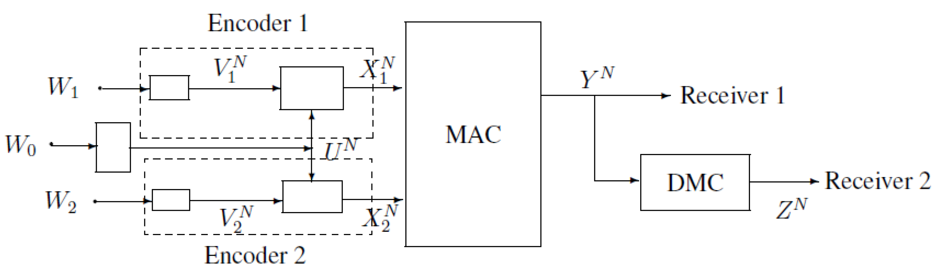
2. Notations, Definitions and the Main Results of MAC-DBC

In this section, a description of the MAC-DBC is given by Definition 1 to Definition 3. The capacity region, ${\mathcal{R}}^{\left(\mathcal{A}\right)}$, composed of all achievable $(R_0,R_1,R_2)$ triples is given in Theorem 2, where the achievable $(R_0,R_1,R_2)$ triple is defined in Definition 4.

Definition 1 

(Encoders) The private messages, $W_1$ and $W_2$, take values in ${\mathcal{W}}_1$ and ${\mathcal{W}}_2$, respectively. The common message, $W_0$, takes values in ${\mathcal{W}}_0$. $W_0$, $W_1$ and $W_2$ are independent and uniformly distributed over their ranges. The channel encoders are two mappings:

$$f_1^N:{\mathcal{W}}_0\times {\mathcal{W}}_1\to {\mathcal{X}}_1^N$$

(1)

where $f_1^N(w_0,w_1)=x_1^N\in {\mathcal{X}}_1^N$, $w_1\in {\mathcal{W}}_1$, and $w_0\in {\mathcal{W}}_0$.

$$f_2^N:{\mathcal{W}}_0\times {\mathcal{W}}_2\to {\mathcal{X}}_2^N$$

(2)

where $f_2^N(w_0,w_2)=x_2^N\in {\mathcal{X}}_2^N$, $w_2\in {\mathcal{W}}_2$, and $w_0\in {\mathcal{W}}_0$. Note that $W_1$ and $X_2^N$ are independent, and $W_2$ is independent of $X_1^N$.

The transmission rates of the private messages and the common message are $\frac{log\parallel {\mathcal{W}}_1\parallel }{N}$, $\frac{log\parallel {\mathcal{W}}_2\parallel }{N}$, and $\frac{log\parallel {\mathcal{W}}_0\parallel }{N}$, respectively.

Definition 2 

(Channels) The MAC is a DMC with finite input alphabet ${\mathcal{X}}_1\times {\mathcal{X}}_2$, finite output alphabet $\mathcal{Y}$ and transition probability $Q_1\left(y\right|x_1,x_2)$, where $x_1\in {\mathcal{X}}_1,x_2\in {\mathcal{X}}_2,y\in \mathcal{Y}$. $Q_1\left(y^N\right|x_1^N,x_2^N)={\prod }_{n=1}^N{Q}_1\left(y_n\right|x_{1,n},x_{2,n})$. The inputs of the MAC are $X_1^N$ and $X_2^N$, while the output is $Y^N$.

Receiver 2 has access to the output of the MAC via a discrete memoryless channel (DMC). The input of this DMC is $Y^N$, and the output is $Z^N$. The transition probability satisfies that

$$p_{Z^N|Y^N}\left(z^N\right|y^N)=\prod _{i=1}^N{p}_{Z|Y}\left(z_i\right|y_i)$$

(3)

where $z_i\in \mathcal{Z}$ and $y_i\in \mathcal{Y}$.

Definition 3 

(Decoders) The decoder for receiver 1 is a mapping, $f_{D1}:{\mathcal{Y}}^N\to {\mathcal{W}}_1\times {\mathcal{W}}_2\times {\mathcal{W}}_0$, with input $Y^N$ and outputs ${\widehat{W}}_1$, ${\widehat{W}}_2$, ${\widehat{W}}_0$. Let $P_{e1}$ be the error probability of the receiver 1 , and it is defined as $Pr\{(W_0,W_1,W_2)\ne ({\widehat{W}}_0,{\widehat{W}}_1,{\widehat{W}}_2)\}$.

The decoder for receiver 2 is a mapping, $f_{D2}:{\mathcal{Z}}^N\to {\mathcal{W}}_0$, with input $Z^N$ and output ${\widehat{W}}_0$. Let $P_{e2}$ be the error probability of the receiver 2 , and it is defined as $Pr\{W_0\ne {\widehat{W}}_0\}$.

Definition 4 

(Achievable $(R_0,R_1,R_2)$ triple in the model of Figure 5) A triple $(R_0,R_1,R_2)$ (where $R_0,R_1,R_2>0$) is called achievable if, for any $ϵ>0$ (where ϵ is an arbitrary small positive real number and $ϵ\to 0$), there exists channel encoders-decoders $(N,P_{e1},P_{e2})$, such that

$$\frac{log\parallel {\mathcal{W}}_0\parallel }{N}\ge R_0-ϵ,\frac{log\parallel {\mathcal{W}}_1\parallel }{N}\ge R_1-ϵ,\frac{log\parallel {\mathcal{W}}_2\parallel }{N}\ge R_2-ϵ,P_{e1}\le ϵ,P_{e2}\le ϵ$$

(4)

Theorem 2 gives a single-letter characterization of the set ${\mathcal{R}}^{\left(\mathcal{A}\right)}$, which is composed of all achievable $(R_0,R_1,R_2)$ triples in the model of Figure 5, and it is proved in Section A and Section B.

Theorem 2 

A single-letter characterization of the region ${\mathcal{R}}^{\left(\mathcal{A}\right)}$ is as follows,

$${\mathcal{R}}^{\left(\mathcal{A}\right)}=\left\{\begin{array}{c}(R_0,R_1,R_2):\hfill \\ 0\le R_0\le I(U;Z)\hfill \\ 0\le R_1\le I(X_1;Y|X_2,U)\hfill \\ 0\le R_2\le I(X_2;Y|X_1,U)\hfill \\ R_0+R_1\le I(X_1,X_2;Y|V_2)\hfill \\ R_0+R_2\le I(X_1,X_2;Y|V_1)\hfill \\ R_1+R_2\le I(X_1,X_2;Y|U)\hfill \\ R_0+R_1+R_2\le I(X_1,X_2;Y).\hfill \end{array}\right\}$$

where $(U,V_1,V_2)\to (X_1,X_2)\to Y\to Z.$

Remark 1 

There are some notes on Theorem 2; see the following.

• The region ${\mathcal{R}}^{\left(\mathcal{A}\right)}$ is convex, and the proof is in Section C.
• The ranges of the random variables U, $V_1$ and $V_2$ satisfy

  $$\parallel \mathcal{U}\parallel \le \parallel {\mathcal{X}}_1\parallel \parallel {\mathcal{X}}_2\parallel +2$$

  $$\parallel {\mathcal{V}}_1\parallel \le \parallel {\mathcal{X}}_1\parallel \parallel {\mathcal{X}}_2\parallel$$

  $$\parallel {\mathcal{V}}_2\parallel \le \parallel {\mathcal{X}}_1\parallel \parallel {\mathcal{X}}_2\parallel$$

  The proof is in Section D.
• The auxiliary random variables U, $V_1$ and $V_2$, in fact, are corresponding to $W_0$, $W_1$ and $W_2$, respectively.
• If $R_0=0$, receiver 2 is useless, and the model of Figure 5 reduces to the multiple-access channel (MAC).
  Let $R_0=0$, and the corresponding $U=const$, the region, ${\mathcal{R}}^{\left(\mathcal{A}\right)}$, reduces to

  $$\left\{\begin{array}{c}(R_1,R_2):\hfill \\ 0\le R_1\le I(X_1;Y|X_2)\hfill \\ 0\le R_2\le I(X_2;Y|X_1)\hfill \\ R_1\le I(X_1,X_2;Y|V_2)\hfill \\ R_2\le I(X_1,X_2;Y|V_1)\hfill \\ R_1+R_2\le I(X_1,X_2;Y).\hfill \end{array}\right\}$$

  (5)

  Note that the Markov chains, $V_1\to X_1\to Y$ and $V_2\to X_2\to Y$, then the inequalities $R_1\le I(X_1,X_2;Y|V_2)$ and $R_2\le I(X_1,X_2;Y|V_1)$ are included in $R_1\le I(X_1;Y|X_2)$ and $R_2\le I(X_2;Y|X_1)$, respectively. Therefore, the above region (5) is simplified as

  $$\left\{\begin{array}{c}(R_1,R_2):\hfill \\ 0\le R_1\le I(X_1;Y|X_2)\hfill \\ 0\le R_2\le I(X_2;Y|X_1)\hfill \\ R_1+R_2\le I(X_1,X_2;Y).\hfill \end{array}\right\}$$

  (6)

  , and this is coincident with the capacity region of the MAC [12,13].

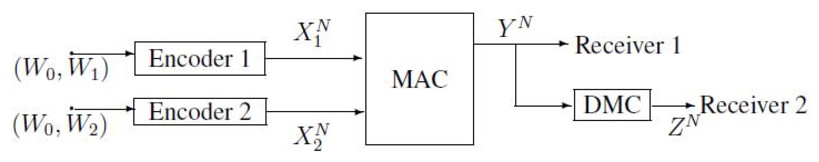
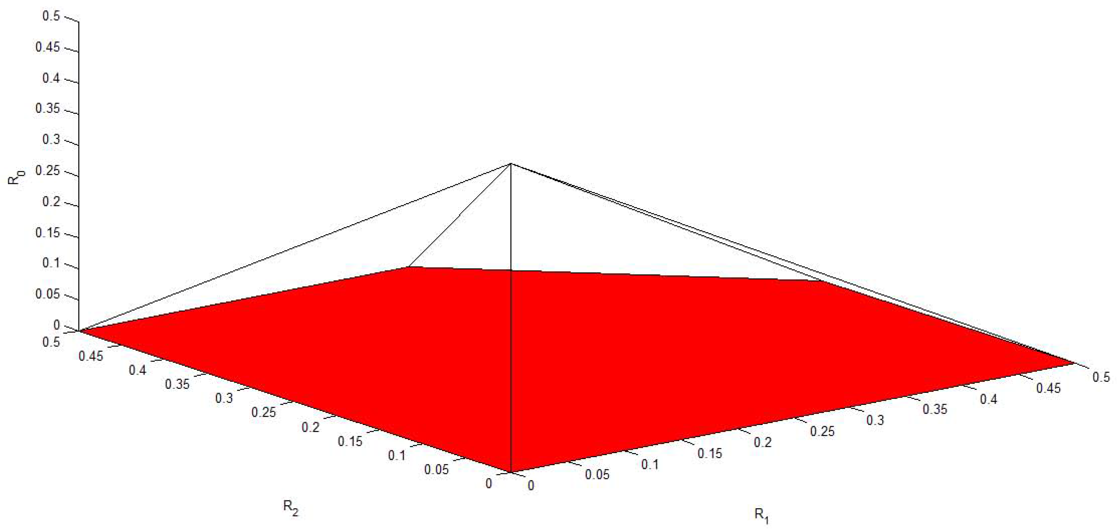
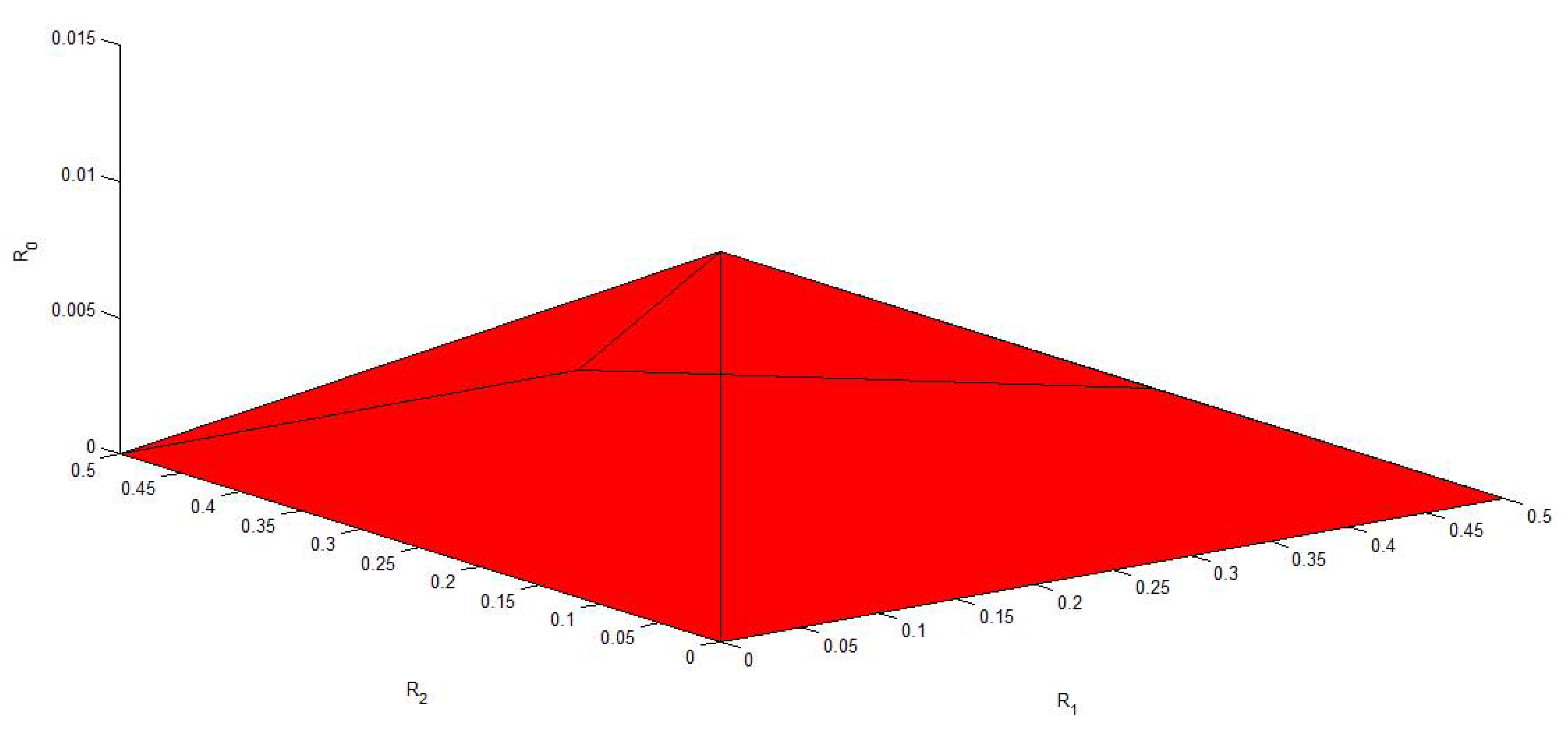
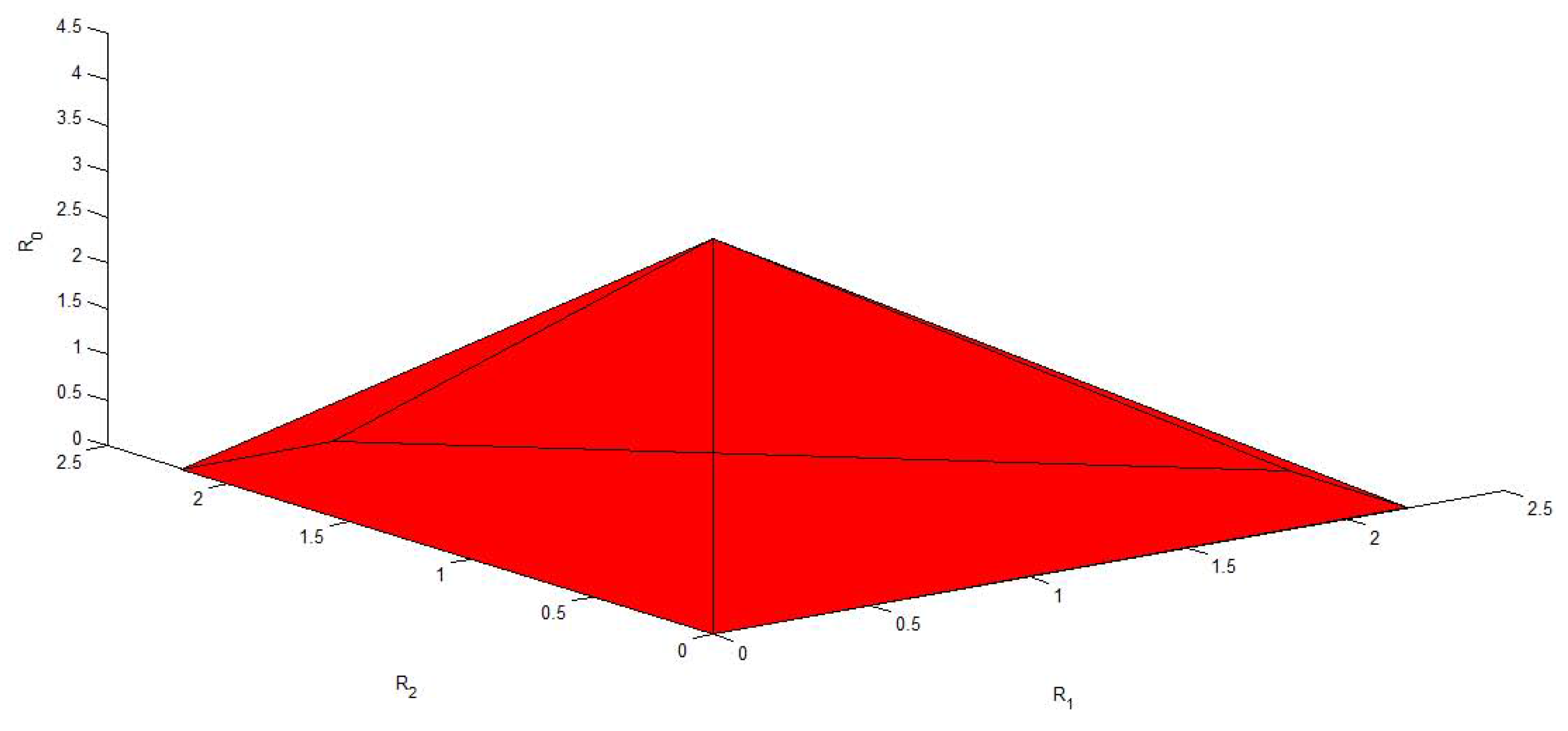
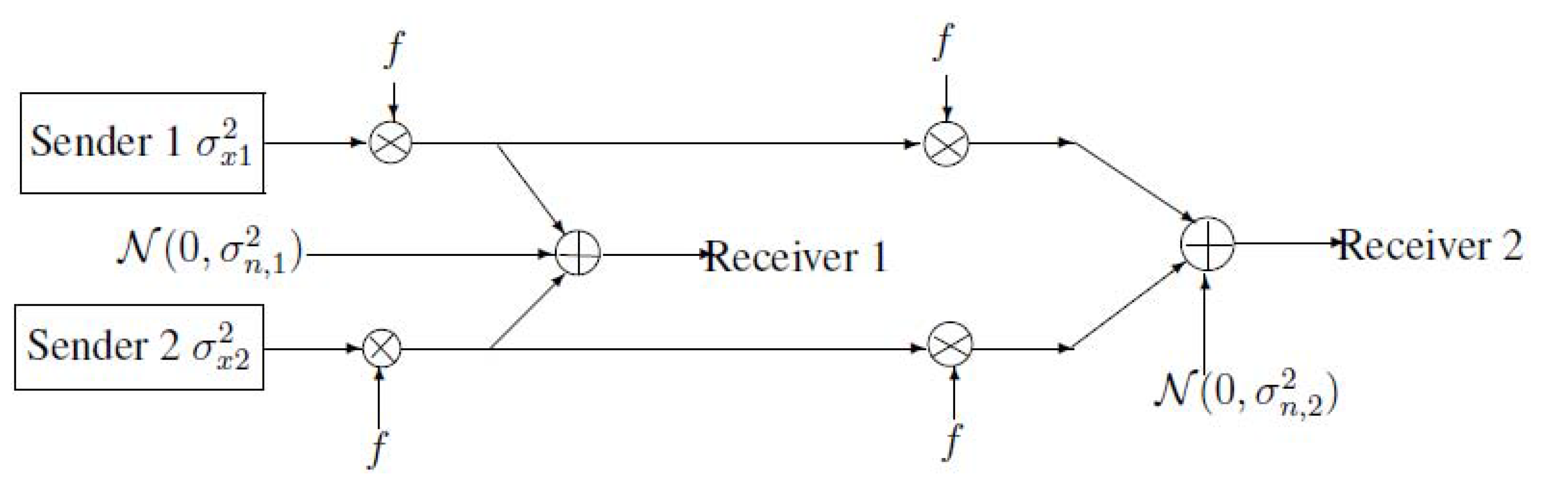
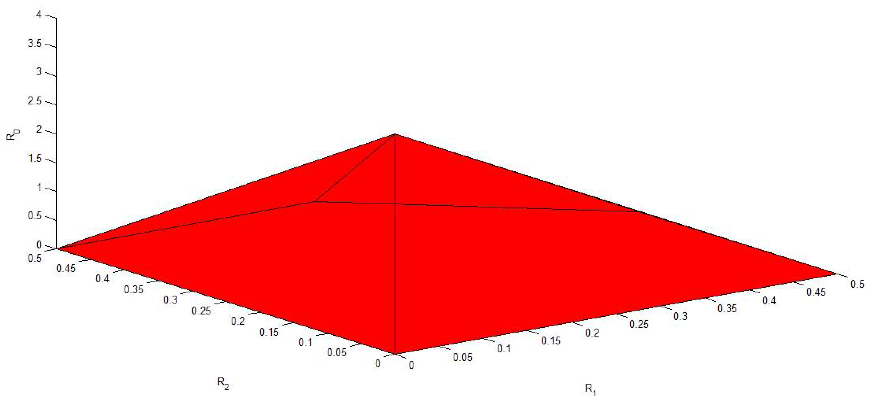
3. A Gaussian Example of MAC-DBC and the Capacity Region of the Model of Figure 4

In this section, we first study a Gaussian example of Figure 5, where the channel input-output relationships at each time instant i ($1\le i\le N$) are given by

$$Y_i=X_{1,i}+X_{2,i}+Z_{1,i}$$

(7)

and

$$Z_i=X_{1,i}+X_{2,i}+Z_{1,i}+Z_{2,i}$$

(8)

where $Z_{1,i}\sim \mathcal{N}(0,{\sigma }_{n,1}^2)$ and $Z_{2,i}\sim \mathcal{N}(0,{\sigma }_{n,2}^2)$. The random vectors, $Z^N$, $Z_1^N$ and $Z_2^N$, are independent with i.i.d. components. The channel inputs, $X_1^N$ and $X_2^N$, are subject to the average power constraints, ${\sigma }_{x,1}^2$ and ${\sigma }_{x,2}^2$, respectively, i.e.,

$$\frac{1}{N}\sum _{i=1}^{N}E\left[X_{1,i}^2\right]\le {\sigma }_{x,1}^2,\frac{1}{N}\sum _{i=1}^{N}E\left[X_{2,i}^2\right]\le {\sigma }_{x,2}^2$$

(9)

Theorem 3 

For the Gaussian case of Figure 5, the capacity-equivocation region, ${\mathcal{R}}^{\left(\mathcal{B}\right)}$, is given by

$${\mathcal{R}}^{\left(\mathcal{B}\right)}=\bigcup _{0\le \alpha \le 1}\left\{\begin{array}{c}(R_0,R_1,R_2):\hfill \\ 0\le R_0\le \frac{1}{2}log(1+\frac{\alpha ({\sigma }_{x,1}^2+{\sigma }_{x,2}^2)}{(1-\alpha )({\sigma }_{x,1}^2+{\sigma }_{x,2}^2)+{\sigma }_{n,1}^2+{\sigma }_{n,2}^2})\hfill \\ 0\le R_1\le \frac{1}{2}log(1+\frac{(1-\alpha ){\sigma }_{x,1}^2}{{\sigma }_{n,1}^2})\hfill \\ 0\le R_2\le \frac{1}{2}log(1+\frac{(1-\alpha ){\sigma }_{x,2}^2}{{\sigma }_{n,1}^2})\hfill \\ R_1+R_2\le \frac{1}{2}log(1+\frac{(1-\alpha )({\sigma }_{x,1}^2+{\sigma }_{x,2}^2)}{{\sigma }_{n,1}^2})\hfill \\ R_0+R_1\le \frac{1}{2}log(1+\frac{{\sigma }_{x,1}^2+\alpha {\sigma }_{x,2}^2}{{\sigma }_{n,1}^2})\hfill \\ R_0+R_2\le \frac{1}{2}log(1+\frac{{\sigma }_{x,2}^2+\alpha {\sigma }_{x,1}^2}{{\sigma }_{n,1}^2})\hfill \\ R_0+R_1+R_2\le \frac{1}{2}log(1+\frac{{\sigma }_{x,1}^2+{\sigma }_{x,2}^2}{{\sigma }_{n,1}^2}).\hfill \end{array}\right\}$$

(10)

The proof of Theorem 3 is in Section E.

Then, we will show that the capacity region of the model of Figure 4 can be obtained from the above Theorem 3. The channel input-output relationships of Figure 4 at each time instant i ($1\le i\le N$) are given by

$$Y_i=f{X}_{1,i}+f{X}_{2,i}+Z_{1,i}$$

(11)

and

$$Z_i=f^2{X}_{1,i}+f^2{X}_{2,i}+Z_{2,i}$$

(12)

, where $Z_{1,i}\sim \mathcal{N}(0,{\sigma }_{n,1}^2)$, $Z_{2,i}\sim \mathcal{N}(0,{\sigma }_{n,2}^2)$ and ${\sigma }_{n,1}^2\le {\sigma }_{n,2}^2$. The channel inputs $X_1^N$ and $X_2^N$, are subject to the average power constraints ${\sigma }_{x,1}^2$ and ${\sigma }_{x,2}^2$, respectively.

Note that the additive Gaussian noise, $Z_{2,i}$, can be viewed as a cascade of $Z_{1,i}$ and $Z_{2,i}^{{}^{\prime }}$, where $Z_{2,i}^{\prime }\sim \mathcal{N}(0,{\sigma }_{n,2}^2-{\sigma }_{n,1}^2)$. Moreover, Equations (11) and (12) are equivalent to Equations (13) and (14), respectively, where

$$Y_i=X_{1,i}+X_{2,i}+\frac{1}{f}{Z}_{1,i}$$

(13)

and

$$Z_i=X_{1,i}+X_{2,i}+\frac{1}{f^2}{Z}_{2,i}$$

(14)

Therefore, the model of Figure 4 is analogous to the above Gaussian example of MAC-DBC. The capacity region is as follows.

Theorem 4 

For the model of Figure 4, the capacity region ${\mathcal{R}}^{\left(\mathcal{C}\right)}$ is given by

$${\mathcal{R}}^{\left(\mathcal{C}\right)}=\bigcup _{0\le \alpha \le 1}\left\{\begin{array}{c}(R_0,R_1,R_2):\hfill \\ 0\le R_0\le \frac{1}{2}log(1+\frac{\alpha f^4({\sigma }_{x,1}^2+{\sigma }_{x,2}^2)}{(1-\alpha )({\sigma }_{x,1}^2+{\sigma }_{x,2}^2)f^4+{\sigma }_{n,2}^2})\hfill \\ 0\le R_1\le \frac{1}{2}log(1+\frac{(1-\alpha ){\sigma }_{x,1}^2{f}^2}{{\sigma }_{n,1}^2})\hfill \\ 0\le R_2\le \frac{1}{2}log(1+\frac{(1-\alpha ){\sigma }_{x,2}^2{f}^2}{{\sigma }_{n,1}^2})\hfill \\ R_1+R_2\le \frac{1}{2}log(1+\frac{(1-\alpha )({\sigma }_{x,1}^2+{\sigma }_{x,2}^2)f^2}{{\sigma }_{n,1}^2})\hfill \\ R_0+R_1\le \frac{1}{2}log(1+\frac{({\sigma }_{x,1}^2+\alpha {\sigma }_{x,2}^2)f^2}{{\sigma }_{n,1}^2})\hfill \\ R_0+R_2\le \frac{1}{2}log(1+\frac{({\sigma }_{x,2}^2+\alpha {\sigma }_{x,1}^2)f^2}{{\sigma }_{n,1}^2})\hfill \\ R_0+R_1+R_2\le \frac{1}{2}log(1+\frac{({\sigma }_{x,1}^2+{\sigma }_{x,2}^2)f^2}{{\sigma }_{n,1}^2}).\hfill \end{array}\right\}$$

(15)

The proof is directly obtained from Theorem 3, and it is omitted here.

Figure 6, Figure 7, Figure 8, Figure 9 and Figure 10 plot the capacity region, ${\mathcal{R}}^{\left(\mathcal{C}\right)}$, with different values of f, ${\sigma }_{x,1}^2$, ${\sigma }_{x,2}^2$, ${\sigma }_{n,1}^2$ and ${\sigma }_{n,2}^2$. It is easy to see that ${\mathcal{R}}^{\left(\mathcal{C}\right)}$ reduces to the capacity region of the Gaussian MAC when $R_0=0$. From these figures, we can see that ${\mathcal{R}}^{\left(\mathcal{C}\right)}$ enlarges as ${\sigma }_{n,2}^1$ and ${\sigma }_{n,2}^2$ decrease. Moreover, for fixed f, ${\sigma }_{n,1}^2$ and ${\sigma }_{n,2}^2$, ${\mathcal{R}}^{\left(\mathcal{C}\right)}$ enlarges as ${\sigma }_{x,1}^2$ and ${\sigma }_{x,2}^2$ increase.

Figure 6. The capacity region of Figure 4 with ${\sigma }_{x,1}^2={\sigma }_{x,2}^2=1$, ${\sigma }_{n,1}^2=1$, ${\sigma }_{n,2}^2=2$ and $f=1$.

Figure 7. The capacity region of Figure 4 with ${\sigma }_{x,1}^2={\sigma }_{x,2}^2=1$, ${\sigma }_{n,1}^2=1$, ${\sigma }_{n,2}^2=100$ and $f=1$.

Figure 8. The capacity region of Figure 4 with ${\sigma }_{x,1}^2={\sigma }_{x,2}^2=1$, ${\sigma }_{n,1}^2=1$, ${\sigma }_{n,2}^2=0.01$ and $f=1$.

Figure 9. The capacity region of Figure 4 with ${\sigma }_{x,1}^2={\sigma }_{x,2}^2=2$, ${\sigma }_{n,1}^2=0.1$, ${\sigma }_{n,2}^2=0.01$ and $f=1$.

Figure 10. The capacity region of Figure 4 with ${\sigma }_{x,1}^2={\sigma }_{x,2}^2=1$, ${\sigma }_{n,1}^2=1$, ${\sigma }_{n,2}^2=2$ and $f=0.5$.

4. Conclusions

In this paper, we first study the discrete memoryless MAC-DBC (the model of Figure 5). The capacity region is totally determined for this new model. Then, we study the model of Figure 4 and show that the capacity region of Figure 4 can be directly obtained from the Gaussian example of the MAC-DBC.

References

- Lampe, L.; Schober, R.; Yiu, S. Distributed space-time block coding for multihop transmission in power line communication networks. IEEE J. Select. Areas Commun. 2006, 24, 1389–1400. [Google Scholar] [CrossRef]
- Bumiller, G.; Lampe, L.; Hrasnica, H. Power line communications for large-scale control and automation systems. IEEE Commun. Mag. 2010, 48, 106–113. [Google Scholar] [CrossRef]
- Lampe, L.; Han Vinck, A.J. On cooperative coding for narrow band PLC networks. Int. J. Electron. Commun. (AEÜ) 2011, 8, 681–687. [Google Scholar] [CrossRef]
- Balakirsky, V.; Vinck, A. Potential performance of PLC systems composed of several communication links. Intl. Symp. Power Line Commun. Appl. Vancouver 2005, 10, 12–16. [Google Scholar]
- Johansson, M.; Nielsen, L. Vehicle applications of controller area network. Tech. Rep. 2003, 7, 27–52. [Google Scholar]
- Cover, T.M. Broadcast channels. IEEE Trans. Inf. Theory 1972, 18, 2–14. [Google Scholar] [CrossRef]
- Körner, J.; Marton, K. General broadcast channels with degraded message sets. IEEE Trans. Inf. Theory 1977, 23, 60–64. [Google Scholar] [CrossRef]
- Gallager, R.G. Capacity and coding for degraded broadcast channels. Probl. Inf. Transm. 1974, 10, 3–14. [Google Scholar]
- Bergmans, P.P. A simple converse for broadcast channels with additive white Gaussian noise. IEEE Trans. Inf. Theory 1974, 20, 279–280. [Google Scholar] [CrossRef]
- Bergmans, P.P. Random coding theorem for broadcast channels with degraded components. IEEE Trans. Inf. Theory 1973, 19, 197–207. [Google Scholar] [CrossRef]
- El Gamal, A.; Cover, T.M. Multiple user information theory. Proc. IEEE 1980, 68, 1466–1483. [Google Scholar] [CrossRef]
- Ahlswede, R. Multiway Communication Channels. In Proceedings of the 2nd International Symposium Information Theory, Tsahkadsor, Armenia, /hlconference date, day and month 1971; pp. 23–52. [Green Version]
- Liao, H.H.J. Multiple access channels. Ph.D. Thesis, University of Hawaii, Honolulu, 1972. [Google Scholar] [Green Version]
- Csisza´r, I.; Körner, J. Information Theory. Coding Theorems for Discrete Memoryless Systems; Academic: London, UK, 1981. [Google Scholar] [Green Version]
- El Gamal, A.; Kim, Y. Lecture notes on network information theory. Available online: http://arxiv.org/abs/1001.3404 (accessed on 20 January 2010). [Green Version]
- Yeung, R.W. Information Theory and Network Coding; Springer: New York, NY, USA, 1981. [Google Scholar] [Green Version]
- Liang, Y.; Poor, H.V. Multiple-access channels with confidential messages. IEEE Trans. Inf. Theory 2008, 54, 976–1002. [Google Scholar] [CrossRef]
Appendix
A. Proof of the Converse Part of Theorem 2
In this section, we establish the converse part of Theorem 2: all the achievable triples are contained in the set , i.e., for any achievable triple, there exists random variables U, , , , , Y and Z such that the inequalities in Theorem 2 hold, and forms a Markov chain. We will prove the inequalities of Theorem 2 in the remainder of this section.
(Proof of ) The proof of this inequality is as follows:
where (a) is from the Fano’s inequality, (b) is from , (c) is from the definition that , (d) is from J as a random variable (uniformly distributed over ), and J is independent of and , (e) is from J as uniformly distributed over , and (f) is from the definitions that and .
Letting and note that , , it is easy to see that .
where (1) is from the Fano’s inequality and the fact that is independent of and ; (2) is from ; (3) is from the discrete memoryless property of the channel; (4) is from ; and (5) is from the definitions that , , , , where J is a random variable (uniformly distributed over ), and is independent of , , , and .
(Proof of ) The proof is similar to the proof of , and it is omitted here.
(Proof of )
where (a) is from the Fano’s inequality and the fact that is independent of and ; (b) is from ; (c) is from the discrete memoryless property of the channel; (d) is from ; and (e) is from the definitions that , , and .
Letting and note that , , and is independent of , it is easy to see that .
(Proof of ) The proof is obtained by the following Equation (A4).
(Proof of ) The proof is analogous to the proof of , and it is omitted here.
where (a) is from the Fano’s inequality; (b) is from ; (c) is from the discrete memoryless property of the channel; and (d) is from the definitions that , , .
Letting and note that , , , , it is easy to see that .
The Markov chain, , is directly obtained from the definitions , , , , and .
The proof of the converse part of Theorem 2 is completed.
B. Proof of the Direct Part of Theorem 2
In this section, we establish the direct part of Theorem 2 (about existence). Suppose , we will show that is achievable.
The coding scheme for Theorem 2 is in the following Figure A1. Now, the remainder of this section is organized as follows. Some preliminaries about typical sequences are introduced in Subsection B.1. The construction of the code is introduced in Subsection B.2. For any given , the proofs of , , , and are given in Subsection B.3.
Figure A1.
Coding scheme for MAC-DBC.
B.1. Preliminaries
- Given a probability mass function, , for any , let be the strong typical set of all , such that for all , where is the number of occurences of the letter v in the . We say that the sequences, , are V-typical.
- Analogously, given a joint probability mass function, , for any , let be the joint strong typical set of all pairs , such that for all and , where is the number of occurences of in the pair of sequences . We say that the pairs of sequences, are -typical.
- Moreover, is called -generated by iff is V- typical and . For any given , define .
- Lemma 1 For any ,where as .
B.2. Coding Construction
Given a triple , choose a joint probability mass function, , such that
The message sets, , and , satisfy the following conditions:
Code-book generation:
- For a given , generate a corresponding i.i.d., according to the probability mass function .
- is generated according to a new discrete memoryless channel (DMC), with inputs and , and output . The transition probability of this new DMC is .Similarly, is generated according to a new discrete memoryless channel (DMC), with inputs and , and output . The transition probability of this new DMC is .
Decoding scheme:
- (Receiver 1) Receiver 1 declares that messages, , and , are sent if they are the unique messages, such that , otherwise, it declares an error.
- (Receiver 2) Receiver 2 declares that a message is sent if it is the unique message, such that ; otherwise it declares an error.
B.3. Achievability Proof
By using the above Equation (A6), it is easy to verify that , and . It remains to show that and ; see the following.
Without loss of generality, assume that , and are sent.
2.3.1.
For receiver 2, define the events:
The probability of error for receiver 2 is then upper bounded by
By using LLN, the first term as . On the other hand, by using the packing lemma [15, p. 53-54], as if .
Therefore, by choosing sufficiently large N, we have .
2.3.2.
The proof of is as follows.
Define the sets
The probability of error for receiver 1 is then upper bounded by:
By using LLN, the first term, as .
For the second term, by using the packing lemma ([15][p. 53–54]), as if
where (1) is from and .
Analogously, for the third term, by using the packing lemma, as if .
For the fourth term, by using the packing lemma, as if .
where (2) is from .
For the fifth term, as if .
For the sixth term, by using the packing lemma, as if
where (3) is from .
Analogously, the seventh term, as if .
For the eighth term, by using the packing lemma, as if .
The proof of the direct part of Theorem 2 is completed.
C. Proof of the Convexity of
Let , i.e., , satisfy the following conditions:
Let Q be a switch function, such that and , where . Q is independent of all the random variables.
Define , , , , , , . Then we have
D. Size Constraints of the Auxiliary Random Variables in Theorem 2
By using the support lemma (see [14], p.310), it suffices to show that the random variables U, A and K can be replaced by new ones, preserving the Markovity and the characters , , , , , , and furthermore, the range of the new U, A and K satisfies:
The proof of which is in the reminder of this section.
Let
Define the following continuous scalar functions of :
Since there are functions of , the total number of the continuous scalar functions of is +2.
Let . With these distributions , we have
According to the support lemma ([14], p.310), the random variable, U, can be replaced by new ones, such that the new U takes at most different values and the expressions (A20)–(A23) are preserved.
Similarly, we can prove that and . The proof is omitted here.
E. Proof of Theorem 3
E.1. Proof of the Achievability
The achievability proof follows by computing the mutual information terms in Theorem 2 with the following joint distributions:
U is independent of and .
E.2. Proof of the Converse
The proof of and are from the proof of the Gaussian broadcast channel [15], and it is omitted here.
The proof of , and are from the proof of the Gaussian multiple-access channel [16], and it is omitted here.
Then, it remains to show that and . The proof of these two inequalities are analogous to ([17] [p. 1000–1001]), and therefore, we omit the proof here.
The proof of Theorem 3 is completed.
© 2013 by the authors; licensee MDPI, Basel, Switzerland. This article is an open access article distributed under the terms and conditions of the Creative Commons Attribution license (http://creativecommons.org/licenses/by/3.0/).