Abstract
We consider two different time fractional telegrapher’s equations under stochastic resetting. Using the integral decomposition method, we found the probability density functions and the mean squared displacements. In the long-time limit, the system approaches non-equilibrium stationary states, while the mean squared displacement saturates due to the resetting mechanism. We also obtain the fractional telegraph process as a subordinated telegraph process by introducing operational time such that the physical time is considered as a Lévy stable process whose characteristic function is the Lévy stable distribution. We also analyzed the survival probability for the first-passage time problem and found the optimal resetting rate for which the corresponding mean first-passage time is minimal.
1. Introduction
Due to economic and military reasons in the XIX-th century, the rapid communication between the countries belonging to the British Empire was an important matter. To send a message from one part of the Empire to another was a true challenge, for its solution contributed to many famous physicists of that time, namely J. Maxwell, Lord Kelvin, and O. Heaviside. Nevertheless, only Heaviside solved this problem. He proposed the so-called telegrapher’s (telegraph) equation (TE) to describe the current propagation inside the telegrapher’s cable []. His equation is a hyperbolic equation which, in -dimensional space, has the following form
where is a time parameter measured in seconds, and v is the propagation velocity measured in seconds/meter. The boundary conditions are set to zero at infinity, while the initial conditions are
These boundary and initial conditions, allowed C. R. Cattaneo [,] and P. Vernotte [] to employ Equation (1) to describe the heat transport. Thus, the physical interpretation of and v is changing. Here, modifies the Fourier law which connects the heat current and the temperature such that we have
The parameter v is associated with heat conductivity. Recently, Equation (1) has been used to characterize the diffusion process with finite propagation velocity v [], where , K is the diffusion coefficient, and the Fourier law is replaced by Fick’s law. In this case, the solution of the telegrapher’s equation is a probability density distribution (PDF) and, for arbitrary initial conditions, is presented in Ref. [] (Equation (102) on p. 303 and/or [] Equation (7.4.28)). This solution for the initial conditions given by Equation (2) reduces to the form
derived in Ref. []. We use the standard notation for which denotes the Heaviside step function, and is the modified Bessel function of the first kind of order . The corresponding mean squared displacement (MSD) reads
which leads to the ballistic time dependence in the short-time regime and to the linear time dependence in the long-time one.
Equation (1) characterizes the telegraph process whose corresponding Langevin equation reads
where v denotes the constant particle speed, and is a stationary dichotomic Markov process that jumps between two states; , with a mean rate [,,,] (, is a time scale that corresponds to the inverse mean sojourn time for each state). As shown in [,] subordinating this process by the Lévy process, we can find the fractional telegrapher’s equation of type I (abbreviated as FTE-I), namely
where and is the fractional derivative in the Caputo sense (see Appendix A). Equation (5) can be interpreted as an anomalous diffusion equation, which can be derived by using the continuity equation with an appropriate modified constitutive relation [].
Despite the compelling generalization given by Equation (5), whose higher fractional derivative is always twice the lower one, it is possible to postulate different kinds of fractional telegrapher’s equations. For instance, we focus on one of these possibilities called type II (abbreviated as FTE-II), which has the form (this form corresponds to Equation (17) in Ref. [])
where . In this case, the higher fractional derivative is always larger than 1. Equations (5) and (6) are completed with the same initial and boundary conditions (2) as for the telegrapher’s Equation (1). We can also find different fractional generalisations of the TE [,,,,,], including non-Markovian discrete time versions of the telegraph process [], TE in random media [,,], telegraph processes with random velocities [], etc.
In this paper, we consider the stochastic resetting of the PDFs and that solve Equations (5) and (6), respectively. The stochastic dynamics of the particle, which are initially located at at , under the effects of stochastic resetting, are described by the renewal equation []
where , indicates the probability density corresponding to the different telegrapher’s equations considered here; is the probability that no renewal has taken place up to time t. We consider here the stochastic Poissonian resetting with probability and from this, we have , where r is the resetting rate. The renewal Equation (7) for Poissonian resetting has the form [,,]:
which, in the Laplace space, reads
Furthermore, we assume that the particle is instantaneously reset to the initial position. These assumptions offer the possibility of analytical calculations, as well a description of the experimental results for the mean-first passage time under stochastic resetting, by using holographic optical tweezers [] or laser traps [].
The paper is organized as follows. In Section 2, we consider the stochastic resetting of FTE-I. For that purpose, we find its solution in two ways based on integral decomposition techniques. This decomposition is rooted in recognizing the Brownian motion or the telegraph process. Next, we will reset the process described by FTE-I and calculate the first-passage time problem and survival probability. In Section 3, we repeat all procedures with the stochastic resetting for FTE-II. The paper is summarized in Section 4. The paper contains four Appendices.
2. FTE-I under Resetting
The PDF can be found in two ways, which come from the Efros theorem (Appendix C) applied to . In the Laplace–Fourier (LF) space, it is written as
Here,
and and are the Laplace and Fourier coordinates, respectively. The Efros theorem allows us to make the integral decomposition of Equation (10), for which we represent as the integral with the Gaussian
and
The function for is non-negative, such that it can be named the PDF of the leading process. Another possibility is to present as the solution of the telegrapher’s equation given by Equation (3) and being for the PDF of the leading process (for details, see Section 2.2). Hence, the solution obtained in this way is called the subordination approach. Both techniques in the presence of stochastic resetting will be described below, and we show that they lead to the same results.
2.1. Resetting of FTE-I—The First Possibility
Let us begin by examining the outcomes that can be derived from the second equality in Equation (10). In the short-time regime, , we have that Equation (10) is approximated by
which, after inverting the Laplace and Fourier transforms, we obtain the fractional wave equation (fWE)
Transport in this regime is described by the fWE. In the opposite regime, i.e., in the long-time regime, , Equation (10) is asymptotically approximated by
which corresponds to the standard fractional diffusion equation (fDE) after inverting the Laplace and Fourier transforms, i.e.,
In the general case, upon performing the Fourier transform inversion of Equation (10), we can express it in Laplace space as:
which, after taking the inverse Laplace transform, can be written in t-space as the generalized diffusion equation
The series representation of the two-parameter Mittag–Leffler function is given by Equation (A1) for . After multiplying the last equation by and integrating over space we are led to first-order differential equations for the MSD, which can be integrated straightforwardly to give . We emphasize that the procedure of expressing the hyperbolic-like Equation (5) as the parabolic-like Equation (19) is only formal and it is possible only for the diffusion-like initial conditions (2). Formally, we can present the solution of Equation (19) as
where and are given by Equations (12) and (13), respectively. The same results can be obtained using Equation (A3) resulting from the Efros theorem in which , , and . In the LF space, it figures as
Note that is a non-negative function for . That comes from the Bernstein theorem [] and the fact that , for this range of , is a completely monotonic function (CMF), i.e., the non-negative function whose derivatives exist and alternate, see Appendix B. In consequence, we can say that , given by Equation (20) for is a PDF expressed by the subordination approach, in which the leading process, described by , subordinates the parent process characterized by the normal distribution [,]. The function for is not a CMF. Then, according to the Bernstein theorem, is negative or contains negative parts. However, calculated from Equation (21) for is a CMF, yielding that its inverse is non-negative and can be called a PDF.
The corresponding MSD can be expressed in terms of the MSD of the normal distribution , we have
from where, by inverse Laplace transform, one finds
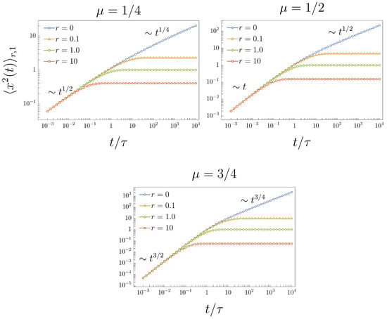
which is a known result []. From (22), we have that in the short-time regime, and in the long-time regime; see Figure 1, curves marked with circle symbols for , 1/2, and 3/4.
If we reset to the initial position according to the stochastic Poissonian resetting , where r is the resetting rate, then the corresponding follows the renewal Equation (8) for . In Laplace space, it reads Equation (9) for , which, after employing Equation (21), gives
From here, we conclude that in the long-time limit, the system approaches the non-equilibrium stationary state (NESS) , which is explicitly given by
The NESS is given by the Laplace distribution with a stationary variance around the average value . For , the NESS is analogous to Equation (27) of Ref. []. For , we recover the result for the NESS for an anomalous diffusion process under resetting [,,,,], i.e., . We want to point out the exponential decay of the NESS tails, which is a characteristic induced by the stochastic Poissonian resetting process.
For the MSD in the case of resetting, we have
from which we obtain
In the short-time limit it behaves as , and in the long-time limit it approaches the constant value,
The graphical representation of the MSD (25) for different values of and r is given in Figure 1, where we observe the asymptotic behavior of the MSD for short- and long-time limits.
2.2. Resetting of FTE-I—The Second Possibility
As mentioned in the Introduction, the FTE-I for can be obtained from the telegraph process subordinated by Lévy noise. Here, we demonstrate this approach, starting from Langevin’s equations:
where represents the same dichotomic noise as in the standard TE, and is a Lévy stable noise with Lévy index in Laplace space given by , . Therefore, the process is a stable Lévy motion with the characteristic function given by the stretched exponential function . Its inverse Laplace transform is denoted as and known as a one-sided Lévy stable distribution whose series form was found by H. Pollard in []. Its representation through the Fox H function was later found by R. Hilfer []. In [], it was presented in the Meijer G form and the finite series of generalized hypergeometric functions. The corresponding PDF of this subordinated telegraph process can be found from the subordination integral [,,,,]
where is the subordination function which, in Laplace space, reads as
Inverting (28), we get the explicit time dependence of the subordination function
This subordination is also obtained from the first equality of Equation (10) by employing the Efros theorem in which , , and [,]. Then, from Equation (A3), we have
whose inverse Laplace transform gives Equation (27). From Equation (29), it follows that the MSD reads
where is the MSD (4) for the standard TE. Therefore, we obtain the same MSD as in Equation (22), as expected. Thus, making the Poissonian resetting as in the previous subsection, we obtain Equation (25); in the long-time limit, this gives Equation (26). Moreover, NESS, given by Equation (23) for this kind of subordination, is also equal to Equation (24).
For , we recover the known results for the standard telegrapher’s equation with stochastic resetting [].
2.3. First-Passage Time Problem
From Equations (18) and (9), we obtain
where, by inverse Laplace transform, the generalized diffusion equation
is obtained, with memory function , where
Let us write the corresponding backward equation for the survival probability , which will give the probability of the particle starting at to reach the target at the origin. Thus, we have
with initial conditions
and boundary conditions and . By Laplace transform, we find that
From here, we can calculate the first-passage time density , i.e., , see [,,], which, in the Laplace space, reads
If we consider the process as a random search, then we can calculate the efficiency of the search, defined as the number of visited targets divided by the average number of steps needed. If there is a single target, it can be calculated as the inverse of the MFPT []
whose derivation is presented in Appendix D.
If we further consider exponential resetting to the telegraph process, then for the survival probability, one finds [,]
from where we derive the MFPT
We see that the MFPT in the limits and diverges, so there is an optimal resetting rate for which MFPT is minimal, i.e.,
from where we have
i.e.,
For it reduces to []
For , we recover the MFPT for the telegraph process under resetting [], see also [],
while for , the result for the subdiffusive search [,]
and for and , the Brownian search with []
The dependence of the MFPT on the resetting rate r is shown in Figure 2, while the optimal resetting rate versus parameter is shown in Figure 3. From Equation (32), for a given exponent , we can numerically find the optimal value r for which the MFPT is minimum, see Figure 3. From Figure 2, we see that by increasing , the resetting rate , for which the MFPT is minimum, decreases. Therefore, we need a higher resetting rate in order to reset the particle, which is stacked due to the long-tailed waiting time, given by the fractional exponent (the lower fractional exponent means a longer waiting time, and therefore, we need a higher resetting rate for the particle to reach the target in a shorter time).
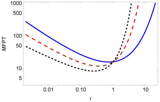
Figure 2.
MFPT (31) for , , , (blue solid line), (red dashed line), (black dotted line).
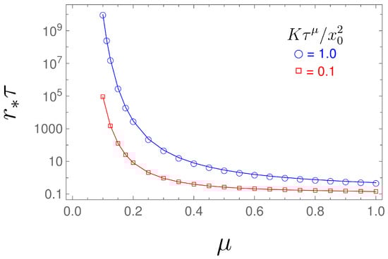
Figure 3.
Optimal resetting rate versus , obtained by numerically solving Equation (32).
3. FTE-II under Resetting
By the same methods used in the previous section, we have that the Laplace transform of Equation (6) looks analogous to Equation (12), but with the difference that instead of , we have to use defined as
Proceeding similarly as in the previous case of FTE-I to obtain Equation (18), we have that
In the short-time regime, we have that the memory function ; therefore, Laplace inversion of Equation (33) is possible since . Thus, we have the fWE
In the long-time regime we recover the fDE
We point out that is not a completely Bernstein function (CBF) since its algebraic inverse is not a Stieltjes function (SF). Formally, we can take the inverse Laplace transform of Equation (33) with initial condition (2), but, due to the results given in Ref. [], it will not be a well-posed Cauchy problem. Hence, we limit our consideration only to the Laplace space in which the solution of Equation (33) can be written as
The MSD corresponding to becomes
from which, by inverse Laplace transform, one finds [] (Equation (24)), namely
In the case of stochastic resetting, we express the renewal equation given by Equation (8) for in Laplace space as
which, in the long-time limit, approaches the NESS equal to
Therefore, the NESS is given by the Laplace distribution, as well, with a stationary variance around the average value . For , NESS reduces to the one for the standard telegrapher’s process under resetting []. For , it turns to the NESS for an anomalous diffusion process under resetting [,,,,].
The corresponding MSD in the case of resetting becomes
that is
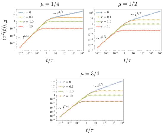
From here, for the short-time limit, we have the behavior , while for the long-time limit we observe saturation
This crossover dynamics of the MSD (38) for different values of and r is shown in Figure 4.
First-Passage Time Problem
We can first solve the backward equation for the survival probability without resetting and then directly find the survival probability with resetting. It reads
with the same initial and boundary conditions as before, we find the survival probability
from where for the first-passage time density we have
The efficiency then becomes
where is the Fox H function in which the argument is given by , and the upper and lower list of parameters reads , , and , respectively. The derivation of the lower formula in Equation (39) is presented in Appendix D.
In the presence of resetting, we can directly find the survival probability from the corresponding one without resetting, from where for the MFPT we obtain
For , we obtain the known result for the MFPT in the case of a standard telegraph process. We can find the optimal resetting rate r for which MFPT is minimal, i.e.,
from where we have
i.e.,
The dependence of the MFPT on the resetting rate is shown in Figure 5, while the changing of the optimal resetting rate by changing parameter is demonstrated in Figure 6. We see that by increasing parameter , the optimal resetting rate decreases, the behavior which was also observed for the FTE-I.
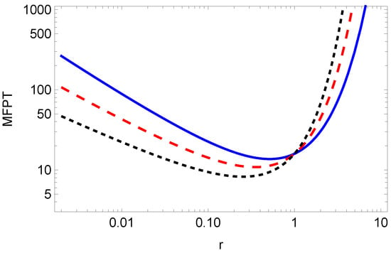
Figure 5.
MFPT (40) for , , , (blue solid line), (red dashed line), (black dotted line).
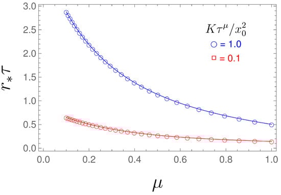
Figure 6.
Optimal resetting rate versus , obtained by numerically solving Equation (41).
4. Summary
In this paper, we considered two distinct kinds of fractional telegrapher equations. In the absence of resetting, we found that both generalizations of the telegrapher equations describe fractional-ballistic transport in the short-time regime, and transit to fractional diffusion transport in the long-time one. FTE-I can be obtained in two ways based on the integral decomposition method, both ways lead to the same results. The methods consist of presenting the solution for the FTE-I from either the normal distribution or from the PDF of the telegraph process. The solution of FTE-II is presented only by use of the normal distribution in the integral decomposition.
Further, we analyzed these two fractional telegraphic processes in the presence of Poissonian resetting, which means that after a random time drawn from an exponential distribution, the particle is reset to the initial position. We found that in the long-time limit, due to the resetting in both cases, the particle reaches non-equilibrium stationary states while the MSDs saturate. In both cases, if the resetting rate is large enough, the nonequilibrium stationary distribution is determined by the short-time regime of the solution of the corresponding FTE, while if the resetting rate is small, the stationary distribution is determined by the long-time regime of the corresponding solution of the FTE.
We also considered the first-passage time problem, and for both cases, we calculated the survival probability, efficiency, and MFPT. It is shown that there is an optimal resetting rate for which the MFPT is minimal. This optimal resetting rate depends on the anomalous diffusion parameter . Additionally, the efficiency in the first case decreases faster with than in the second case.
Analysis of the generalized telegraph processes under non-instantaneous resetting [,,], partial resetting [,], and resetting in an interval [,,] are left for future investigation. The first-passage time problem could also be of interest in the case of resetting to multiple [] and random positions []. Finding the connection between the Shannon and Fisher functionals [] could also be of interest to future research.
Author Contributions
Conceptualization, K.G., F.J.S., G.C.-A. and T.S.; methodology, K.G., F.J.S., G.C.-A. and T.S.; software, K.G., F.J.S., G.C.-A. and T.S.; validation, K.G., F.J.S., G.C.-A. and T.S.; formal analysis, K.G., F.J.S., G.C.-A. and T.S.; investigation, K.G., F.J.S., G.C.-A. and T.S.; writing—original draft preparation, K.G., F.J.S., G.C.-A. and T.S.; writing—review and editing, K.G., F.J.S., G.C.-A. and T.S.; visualization, K.G., F.J.S., G.C.-A. and T.S.; supervision, K.G., F.J.S., G.C.-A. and T.S. All authors have read and agreed to the published version of the manuscript.
Funding
This work was supported by UNAM-PAPIIT IN112623. TS is supported by the German Science Foundation (DFG, Grant number ME 1535/12-1) and by the Alliance of International Science Organizations (Project No. ANSO-CR-PP-2022-05). TS is also supported by the Alexander von Humboldt Foundation. K.G. acknowledges the NCN Research Grant Preludium Bis 2 No. UMO-2020/39/O/ST2/01563.
Data Availability Statement
No new data were created or analyzed in this study. Data sharing is not applicable to this article.
Acknowledgments
K.G. and T.S. acknowledge the hospitality and support from the Lorentz Center in Leiden.
Conflicts of Interest
The authors declare no conflicts of interest.
Abbreviations
The following abbreviations are used in this manuscript:
| TE | Telegrapher’s Equation |
| FTE | Fractional Telegrapher’s Equation |
| MSD | Mean Squared Displacement |
| MFPT | Mean First-Passage Time |
Appendix A. Fractional Calculus and Mittag–Leffler Functions
The fractional derivative in the Caputo sense reads
The three-parameter Mittag–Leffler function is defined by []
Its Laplace transform reads
where . Note that for , it becomes the two parameter Mittag–Leffler function, , and for , it becomes the one parameter Mittag–Leffler function, .
The Fox H function is defined through the Mellin transform as follows
where the parameters are subject to conditions
Appendix B. Completely Monotone and Bernstein Functions
Among the non-negative functions, we can distinguish the complete monotone and Bernstein functions. Based on [], their definitions and subclasses are given below.
A function is a completely monotone function (CMF) if its derivatives exist and , for all .
The important feature of CMF is that the Bernstein theorem uniquely connects it with a non-negative function through the Laplace integral
A (non-negative) Stieltjes function (SF) is a function which can be written as
where and is a measure on such that . Note that the class of SFs belongs to the class of CMFs, and thus, it is a decreasing function. Usually, it is assumed that and , which simplifies the calculations and ensures its integrability at zero and vanishing at infinity.
A function is a Bernstein function (BF) if its all derivatives exist, is non-negative, is a CMF. If a BF , and, additionally, is an SF, then it is called a completely Bernstein function (CBF).
The characteristics of these functions and their properties can be referenced in []. The key features highlighted in this paper include (i) the product or sum of CMFs results in another CMF; (ii) the composition of CMF and BF(CBF) yields a CMF; (iii) for the CBF, there exists a corresponding partner such that ; and (iv) the algebraic inverse of SF (CBF) is CBF (SF).
Appendix C. Efros Theorem
The Efros theorem [,,,,] generalizes the convolution theorem for the Laplace transform. It states the following:
Theorem A1.
If and are analytic functions, and
as well as
exist, then
From Efros theorem appears that
Appendix D. Derivation of the Efficiencies and
The derivation of and base on using the Laplace transform of the Lévy–Smirnov distribution , this is
Inserting it into Equation (30) with and into Equation (39) with , and next changing the order of integrals we get
The auxiliary integral for the efficiencies respectively read
At first, we calculate by setting , which can be expressed as
where we used [] (Equation (2.2.1.16)). The parabolic cylinder function is standard denoted as . Then, we substitute Equation (A5) into Equation (A4) and change onto . That leads to
which, after using [] (Equation (2.11.4.4)), gives the lower formula in Equation (30).
Proceeding analogically, we derive the explicit form of . Now, setting , we can present as
This integral can be calculated for fractional , such that by employing [] (Equation (2.2.1.22)) and then transforming the results into the more transparent language of the Fox H function according to formula [] (Equation (8.3.2.22)). That gives
which substitutes into Equation (A4) for and after changing onto yields
where we used [] (Equation (2.25.2.3)). Next, applying [] (Equation (8.3.1.8)) allows us to get the lower formula in Equation (39).
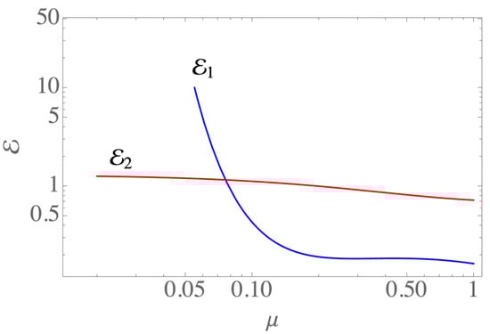
A comparison of the expressions for the efficiencies in each case as a function of is shown in Figure A1. In the FTE-I case, the efficiency decreases with , ranging from high values for small to low values for close to one. In contrast, in the FTE-II case, although efficiency decreases with , it is maintained close to 1 for the whole range of values.
References
- Heaviside, O. On induction between parallel wires. J. Soc. Telegr. Eng. 1880, 9, 427–458. [Google Scholar] [CrossRef]
- Cattaneo, C.R. Sulla conduzione del calore. Atti. Sem. Mat. Fis. Univ. Modena 1948, 3, 83. [Google Scholar]
- Cattaneo, C.R. Sur une forme de l’equation de la chaleur eliminant le paradoxe d’une propagation instantanee’. C. R. Acad. Sci. Paris 1958, 247, 431. [Google Scholar]
- Vernotte, P. Les paradoxes de la théories continue de l’equation de la chaleur. C. R. Acad. Sci. Paris 1958, 246, 3154–3155. [Google Scholar]
- Górska, K.; Horzela, A.; Lenzi, E.K.; Pagnini, G.; Sandev, T. Generalized Cattaneo (telegrapher’s) equations in modeling anomalous diffusion phenomena. Phys. Rev. E 2020, 102, 022128. [Google Scholar] [CrossRef] [PubMed]
- Stratton, J.A. Electromagnetic Theory; McGraw-Hill Book Co.: New York, NY, USA, 1941. [Google Scholar]
- Morse, P.M.; Feshbach, H. Methods of Theoretical Physics; McGraw-Hill Book Co.: New York, NY, USA, 1953. [Google Scholar]
- Masoliver, J. Telegraphic processes with stochastic resetting. Phys. Rev. E 2019, 99, 012121. [Google Scholar] [CrossRef] [PubMed]
- Masoliver, J.; Weiss, G.H. Finite-velocity diffusion. Eur. J. Phys. 1996, 17, 190. [Google Scholar] [CrossRef]
- Masoliver, J.; Lindenberg, K. Continuous time persistent random walk: A review and some generalizations. Eur. J. Phys. B 2017, 90, 107. [Google Scholar] [CrossRef]
- Kac, M. A stochastic model related to the telegrapher’s equation. Rocky Mt. J. Math. 1974, 4, 497. [Google Scholar] [CrossRef]
- Weiss, G.H. Some applications of persistent random walks and the telegrapher’s equation. Phys. A 2002, 311, 381. [Google Scholar] [CrossRef]
- Górska, K.; Horzela, A. Subordination and memory dependent kinetics in diffusion and relaxation phenomena. Fract. Calc. Appl. Anal. 2023, 26, 480. [Google Scholar] [CrossRef]
- Górska, K. Integral decomposition for the solutions of the generalized Cattaneo equation. Phys. Rev. E 2021, 104, 024113. [Google Scholar] [CrossRef] [PubMed]
- Compte, A.; Metzler, R. The generalized Cattaneo equation for the description of anomalous transport processes. J. Phys. A Math. Gen. 1997, 30, 7277–7289. [Google Scholar] [CrossRef]
- Kosztołowicz, T. Cattaneo-type subdiffusion-reaction equation. Phys. Rev. E 2014, 90, 042151. [Google Scholar] [CrossRef] [PubMed]
- D’Ovidio, M.; Polito, F. Fractional Diffusion—Telegraph Equations and Their Associated Stochastic Solutions. Theory Probab. Appl. 2018, 62, 552–574. [Google Scholar] [CrossRef]
- Awad, E.; Metzler, R. Crossover dynamics from superdiffusion to subdiffusion: Models and solutions. Fract. Calc. Appl. Anal. 2020, 23, 55–102. [Google Scholar] [CrossRef]
- Michelitsch, T.M.; Polito, F.; Riascos, A.P. Squirrels can remember little: A random walk with jump reversals induced by a discrete-time renewal process. Commun. Nonlinear Sci. Numer. Simul. 2023, 118, 107031. [Google Scholar] [CrossRef]
- Cáceres, M.O. Finite-velocity diffusion in random media. J. Stat. Phys. 2020, 179, 729–747. [Google Scholar] [CrossRef]
- Cáceres, M.O. Localization of plane waves in the stochastic telegrapher’s equation. Phys. Rev. E 2022, 105, 014110. [Google Scholar] [CrossRef]
- Cáceres, M.O.; Nizama, M. Stochastic telegrapher’s approach for solving the random Boltzmann-Lorentz gas. Phys. Rev. E 2022, 105, 044131. [Google Scholar] [CrossRef]
- Stadje, W.; Zacks, S. Telegraph processes with random velocities. J. Appl. Probab. 2004, 41, 665–678. [Google Scholar] [CrossRef]
- Masó-Puigdellosas, A.; Campos, D.; Méndez, V. Transport properties and first-arrival statistics of random motion with stochastic reset times. Phys. Rev. E 2019, 99, 012141. [Google Scholar] [CrossRef] [PubMed]
- Evans, M.R.; Majumdar, S.N. Diffusion with resetting in arbitrary spatial dimension. J. Phys. A Math. Theor. 2014, 47, 285001. [Google Scholar] [CrossRef]
- Bodrova, A.S.; Chechkin, A.V.; Sokolov, I.M. Scaled Brownian motion with renewal resetting. Phys. Rev. E 2019, 100, 012120. [Google Scholar] [CrossRef] [PubMed]
- Tal-Friedman, O.; Pal, A.; Sekhon, A.; Reuveni, S.; Roichman, Y. Experimental realization of diffusion with stochastic resetting. J. Phys. Chem. Lett. 2020, 11, 7350–7355. [Google Scholar] [CrossRef] [PubMed]
- Besga, B.; Bovon, A.; Petrosyan, A.; Majumdar, S.N.; Ciliberto, S. Optimal mean first-passage time for a Brownian searcher subjected to resetting: Experimental and theoretical results. Phys. Rev. Res. 2020, 2, 032029. [Google Scholar] [CrossRef]
- Schilling, R.L.; Song, R.; Vondraček, Z. Bernstein Functions: Theory and Applications; Walter de Gruyter: Berlin, Germany, 2009. [Google Scholar]
- Masoliver, J.; Montero, M. Anomalous diffusion under stochastic resettings: A general approach. Phys. Rev. E 2019, 100, 042103. [Google Scholar] [CrossRef] [PubMed]
- Kuśmierz, Ł.; Gudowska-Nowak, E. Subdiffusive continuous-time random walks with stochastic resetting. Phys. Rev. E 2019, 99, 052116. [Google Scholar] [CrossRef] [PubMed]
- Stanislavsky, A.; Weron, A. Optimal non-Gaussian search with stochastic resetting. Phys. Rev. E 2021, 104, 014125. [Google Scholar] [CrossRef] [PubMed]
- Singh, R.K.; Gorska, K.; Sandev, T. General approach to stochastic resetting. Phys. Rev. E 2022, 105, 064133. [Google Scholar] [CrossRef] [PubMed]
- Pollard, H. The representation of e−xλ as a Laplace integral. Bull. Am. Math. Soc. 1946, 52, 908. [Google Scholar] [CrossRef]
- Hilfer, R. H-function representations for stretched exponential relaxation and non-Debye susceptibilities in glassy systems. Phys. Rev. E 2002, 65, 061510. [Google Scholar] [CrossRef] [PubMed]
- Penson, K.A.; Górska, K. Exact and Explicit Probability Densities for One-Sided Lévy Stable Distributions. Phys. Rev. Lett. 2010, 105, 210604. [Google Scholar] [CrossRef] [PubMed]
- Fogedby, H.C. Langevin equations for continuous time Lévy flights. Phys. Rev. E 1994, 50, 1657. [Google Scholar] [CrossRef] [PubMed]
- Baule, A.; Friedrich, R. Joint probability distributions for a class of non-Markovian processes. Phys. Rev. E 2005, 71, 026101. [Google Scholar] [CrossRef] [PubMed]
- Chechkin, A.V.; Hofmann, M.; Sokolov, I.M. Continuous-time random walk with correlated waiting times. Phys. Rev. E 2009, 80, 031112. [Google Scholar] [CrossRef] [PubMed]
- Redner, S. A Guide to First-Passage Processes; Cambridge University Press: Cambridge, UK, 2001. [Google Scholar]
- Bray, A.J.; Majumdar, S.N.; Schehr, G. Persistence and first-passage properties in nonequilibrium systems. Adv. Phys. 2013, 62, 225–361. [Google Scholar] [CrossRef]
- Pal, A.; Kundu, A.; Evans, M.R. Diffusion under time-dependent resetting. J. Phys. A Math. Theor. 2016, 49, 225001. [Google Scholar] [CrossRef]
- Palyulin, V.V.; Chechkin, A.V.; Metzler, R. Space-fractional Fokker–Planck equation and optimization of random search processes in the presence of an external bias. J. Stat. Mech. 2014, 2014, P11031. [Google Scholar] [CrossRef]
- Pal, A.; Stojkoski, V.; Sandev, T. Random resetting in search problems. arXiv 2023, arXiv:2310.12057. [Google Scholar]
- Sandev, T.; Kocarev, L.; Metzler, R.; Chechkin, A. Stochastic dynamics with multiplicative dichotomic noise: Heterogeneous telegrapher’s equation, anomalous crossovers and resetting. Chaos Solitons Fractals 2022, 165, 112878. [Google Scholar] [CrossRef]
- Shkilev, V. Continuous-time random walk under time-dependent resetting. Phys. Rev. E 2017, 96, 012126. [Google Scholar] [CrossRef] [PubMed]
- Evans, M.E.; Majumdar, S.N. Diffusion with stochastic resetting. Phys. Rev. Lett. 2011, 106, 160601. [Google Scholar] [CrossRef] [PubMed]
- Kochubei, A.N. General Fractional Calculus, Evolution Equations, and Renewal Processes. Integral Equ. Oper. Theory 2011, 71, 583–600. [Google Scholar] [CrossRef]
- Bodrova, A.S.; Sokolov, I.M. Resetting processes with noninstantaneous return. Phys. Rev. E 2020, 101, 052130. [Google Scholar] [CrossRef]
- Tucci, G.; Gambassi, A.; Majumdar, S.N.; Schehr, G. First-passage time of run-and-tumble particles with noninstantaneous resetting. Phys. Rev. E 2022, 106, 044127. [Google Scholar] [CrossRef] [PubMed]
- Radice, M. One-dimensional telegraphic process with noninstantaneous stochastic resetting. Phys. Rev. E 2021, 104, 044126. [Google Scholar] [CrossRef] [PubMed]
- Tal-Friedman, O.; Roichman, Y.; Reuveni, S. Diffusion with partial resetting. Phys. Rev. E 2022, 106, 054116. [Google Scholar] [CrossRef]
- Di Bello, C.; Chechkin, A.V.; Hartmann, A.K.; Palmowski, Z.; Metzler, R. Time-dependent probability density function for partial resetting dynamics. New J. Phys. 2023, 25, 082002. [Google Scholar] [CrossRef]
- Christou, C.; Schadschneider, A. Diffusion with resetting in bounded domains. J. Phys. A Math. Theor. 2015, 48, 285003. [Google Scholar] [CrossRef]
- Pal, A.; Prasad, V. First passage under stochastic resetting in an interval. Phys. Rev. E 2019, 99, 032123. [Google Scholar] [CrossRef] [PubMed]
- Tucci, G.; Gambassi, A.; Gupta, S.; Roldán, É. Controlling particle currents with evaporation and resetting from an interval. Phys. Rev. Res. 2020, 2, 043138. [Google Scholar] [CrossRef]
- Julián-Salgado, P.; Dagdug, L.; Boyer, D. Diffusion with two resetting points. Phys. Rev. E 2024, 109, 024134. [Google Scholar] [CrossRef] [PubMed]
- Mendez, V.; Flaquer-Galmés, R.; Campos, D. First-passage time of a Brownian searcher with stochastic resetting to random positions. Phys. Rev. E 2024, 109, 044134. [Google Scholar] [CrossRef] [PubMed]
- Cáceres, M.O.; Nizama, M.; Pennini, F. Fisher and Shannon Functionals for Hyperbolic Diffusion. Entropy 2023, 25, 1627. [Google Scholar] [CrossRef] [PubMed]
- Prabhakar, T.R. A singular integral equation with a generalized Mittag Leffler function in the kernel. Yokohama Math. J. 1971, 19, 7. [Google Scholar]
- Efros, A.M. The application of the operational calculus to the analysis. in Russian. Mat. Sborni 1935, 42, 699. [Google Scholar]
- Włodarski, L. Sur une formule de Efros. Stud. Math. 1952, 13, 183. [Google Scholar] [CrossRef]
- Graf, U. Applied Laplace Transforms and z-Transforms for Sciences and Engineers; Birkhäuser: Basel, Switzerland, 2004. [Google Scholar]
- Górska, K.; Penson, K.A. Lévy stable distributions via associated integral transform. J. Math. Phys. 2012, 53, 053302. [Google Scholar] [CrossRef]
- Apelblat, A.; Mainardi, F. Application of the Efros theorem to the function represented by the inverse Laplace transform of s−μexp(-sν). Symmetry 2021, 13, 354. [Google Scholar] [CrossRef]
- Prudnikov, A.P.; Brychkov, Y.A.; Marichev, O.I. Integrals and Series. Direct Laplace Transforms; Gordon and Breach: London, UK, 1992; Volume 4. [Google Scholar]
- Prudnikov, A.P.; Brychkov, Y.A.; Marichev, O.I. Integrals and Series. Special Functions; Taylor & Francis: Abingdon, UK, 1998; Volume 2. [Google Scholar]
- Prudnikov, A.P.; Brychkov, Y.A.; Marichev, O.I. Integrals and Series. More Special Functions; Gordon and Breach: London, UK, 1990; Volume 3. [Google Scholar]
Disclaimer/Publisher’s Note: The statements, opinions and data contained in all publications are solely those of the individual author(s) and contributor(s) and not of MDPI and/or the editor(s). MDPI and/or the editor(s) disclaim responsibility for any injury to people or property resulting from any ideas, methods, instructions or products referred to in the content. |
© 2024 by the authors. Licensee MDPI, Basel, Switzerland. This article is an open access article distributed under the terms and conditions of the Creative Commons Attribution (CC BY) license (https://creativecommons.org/licenses/by/4.0/).