Mathematical Modeling of Linear Fractional Oscillators

Abstract

In this work, based on Newton’s second law, taking into account heredity, an equation is derived for a linear hereditary oscillator (LHO). Then, by choosing a power-law memory function, the transition to a model equation with Gerasimov–Caputo fractional derivatives is carried out. For the resulting model equation, local initial conditions are set (the Cauchy problem). Numerical methods for solving the Cauchy problem using an explicit non-local finite-difference scheme (ENFDS) and the Adams–Bashforth–Moulton (ABM) method are considered. An analysis of the errors of the methods is carried out on specific test examples. It is shown that the ABM method is more accurate and converges faster to an exact solution than the ENFDS method. Forced oscillations of linear fractional oscillators (LFO) are investigated. Using the ABM method, the amplitude–frequency characteristics (AFC) were constructed, which were compared with the AFC obtained by the analytical formula. The Q-factor of the LFO is investigated. It is shown that the orders of fractional derivatives are responsible for the intensity of energy dissipation in fractional vibrational systems. Specific mathematical models of LFOs are considered: a fractional analogue of the harmonic oscillator, fractional oscillators of Mathieu and Airy. Oscillograms and phase trajectories were constructed using the ABM method for various values of the parameters included in the model equation. The interpretation of the simulation results is carried out.

1. Introduction

Models of oscillatory systems (oscillators) are used in various fields of knowledge from mechanics to economics and biology [1,2,3]. From the point of view of mathematics, these models are traditionally described using ordinary differential equations of the second order and the corresponding initial conditions, i.e., the Cauchy problem is posed [1]. It should be noted that such mathematical models cannot take into account the properties of the environment, for example, heredity or memory effect. This effect is characterized by the fact that the oscillating medium can “remember” the impact on it for a long time.

For the first time, the model of the hereditary oscillator was presented in his work by the Italian mathematician V. Volterra [4]. He proposed to take into account heredity in the linear oscillator model using an integro-differential equation with a difference kernel, which he later called the function of heredity or memory. It should be noted that V. Volterra derived the total energy conservation law for this generalized oscillator, in the formula of which an additional term appeared, which is responsible for the dissipation of its energy. This important result was confirmed in subsequent works on this topic.

If we choose a power-law memory function, then we can, using the mathematical apparatus of fractional calculus [5,6,7], go to other model equations that contain derivatives of fractional orders. In this case, the orders of fractional derivatives, as shown by the results of [8,9], will be responsible for the intensity of energy dissipation and are related to the Q-factor of the oscillator. Oscillators with such a description are usually called fractional.

Research methods for mathematical models of fractional oscillators can be divided into exact and numerical. Exact methods, for example, include integral transformations [10] or decomposition methods [11], and numerical methods include the theory of finite-difference schemes [12], variational-iterative methods [11].

In this paper, we will carry out a numerical analysis of mathematical models of linear fractional oscillators (LFO) using elements of the theory of finite-difference schemes. As methods of numerical analysis, we will choose a method based on an explicit non-local finite-difference scheme (ENFDS) studied in the author’s work [13] and the fractional ABM method, which was investigated in [14,15,16]. Let us analyze the errors of the methods using Runge’s rule, and obtain the calculated curves of oscillograms and phase trajectories of the Mathieu, Airy LFOs and an analogue of a harmonic oscillator. Let us investigate the forced oscillations of the LFO and give an interpretation of the research results.

2. Preliminary Material on Fractional Calculus

Here we will consider the basic definitions from the theory of fractional calculus; its aspects can be studied in more detail in the books [5,6,7].

Definition 1.

Fractional Riemann–Liouville integral of order α:

$$I_{0t}^{\alpha }x\left(\tau \right)=\frac{1}{\mathsf{\Gamma }\left(\alpha \right)}\underset{0}{\overset{t}{\int }}\frac{x\left(\tau \right)d\tau }{{\left(t-\tau \right)}^{1-\alpha }},\alpha >0,t>0,$$

(1)

where $\mathsf{\Gamma }\left(\alpha \right)={\int }_0^{\infty }{t}^{\alpha -1}{e}^{-t}dt,Re\left(\alpha \right)>0$ is Euler’s gamma function.

The operator (1) has the following properties:

$$I_{0t}^{0}x\left(\tau \right)=x\left(t\right),I_{0t}^{\alpha }{I}_0^{\beta }x\left(\tau \right)=I_{0t}^{\alpha +\beta }x\left(\tau \right),I_{0t}^{\alpha }{I}_0^{\beta }x\left(\tau \right)=I_0^{\beta }{I}_{0t}^{\alpha }x\left(\tau \right).$$

Definition 2.

The fractional Gerasimov–Caputo derivative of order α has the form:

$${\partial }_{0t}^{\alpha }x\left(\tau \right)=\left\{\begin{array}{c}{\displaystyle \frac{1}{\mathsf{\Gamma }\left(m-\alpha \right)}}\underset{0}{\overset{t}{\int }}{\displaystyle \frac{x^{\left(m\right)}\left(\tau \right)d\tau }{{\left(t-\tau \right)}^{\alpha +1-m}}},0\le m-1<\alpha <m,\hfill \\ {\displaystyle \frac{d^{m}x\left(t\right)}{d{t}^m}},m\in N.\hfill \end{array}\right.$$

(2)

The operator (2) has the following properties [5]:

$${\partial }_{0t}^{\alpha }{I}_{0t}^{\alpha }x\left(\tau \right)=x\left(t\right),I_{0t}^{\alpha }{\partial }_{0t}^{\alpha }x\left(\tau \right)-\sum _{k=0}^{i-1}\frac{x^{\left(k\right)}\left(0\right)t^k}{k!},t>0.$$

3. Generalization of Newton’s Second Law

Consider a mechanical system that takes into account dynamic memory in the presence of dissipation. Let us write the equation of motion for such a system in the form:

$$m\dot{x}\left(t\right)=\underset{0}{\overset{t}{\int }}G\left(t-\tau \right)F\left(x\left(\tau \right),\tau \right)d\tau$$

(3)

where $F\left(x,\tau \right)$ is the resultant of all forces acting on a material body with mass m, $G\left(t-\tau \right)$ is a memory function that characterizes the change impulse of a mechanical system as a reaction to the initial action of a force.

In the case when the mechanical system does not have dissipation, the memory function is the Heaviside function, which corresponds to ideal memory. In this case, the momentum of the system does not change upon the initial action of the force. The presence of dissipation in the system leads to a gradual forgetting, the initial impact exerted on it, while the simplest form of the dynamic memory function can be described by the relation [17]:

$$G\left(t\right)=\frac{1}{\mathsf{\Gamma }\left(\alpha \right)t^{1-\alpha }},0<\alpha <1,$$

(4)

where $\alpha$ is the intensity of dissipation, for $\alpha =1$ there is no dissipation.

Substituting relation (4) into (3) and taking into account the definition of the fractional Riemann–Liouville integral (1), we have

$$m\dot{x}\left(t\right)=\frac{1}{\mathsf{\Gamma }\left(\alpha \right)}\underset{0}{\overset{t}{\int }}\frac{F\left(x\left(\tau \right),\tau \right)}{{\left(t-\tau \right)}^{1-\alpha }}d\tau =I_{0t}^{\alpha }F\left(x,\tau \right),$$

(5)

Next, we invert the fractional integral in (5) using the composition property:

$$m{\partial }_{0t}^{\alpha }\dot{x}\left(t\right)={\partial }_{0t}^{\alpha }{I}_{0t}^{\alpha }F\left(x,\tau \right)=F\left(x,t\right),{\partial }_{0t}^{\alpha }\dot{x}\left(\tau \right)={\partial }_{0t}^{1+\alpha }x\left(\tau \right)=\frac{1}{\mathsf{\Gamma }\left(1-\alpha \right)}\underset{0}{\overset{t}{\int }}\frac{\ddot{x}\left(\tau \right)}{{\left(t-\tau \right)}^{\alpha }}d\tau .$$

(6)

As a result, taking into account relation (6), we arrive at the equation:

$$m{\partial }_{0t}^{\beta }x\left(\tau \right)=F\left(x,t\right),\beta =1+\alpha .$$

(7)

Equation (7) is a generalization of Newton’s second law and coincides with it for $\beta =2$.

Depending on the right side of this equation—the form of the function $F\left(x,t\right)$, we will obtain model equations of oscillatory systems with memory. In this paper, we will consider a wide class of oscillatory systems with dynamic memory, when the right-hand side can be represented as:

$$F\left(x,t\right)=f\left(t\right)-\omega \left(t\right)x\left(t\right)-\lambda {\partial }_{0t}^{\gamma }x\left(\tau \right),0<\gamma <1,$$

(8)

here $f\left(t\right)$ is the external action, $\omega \left(t\right)$ is the natural oscillation frequency, $\lambda$ is the viscous friction coefficient.

Let $m=1$ for simplicity. Taking into account (8), let us formulate the following problem statement.

4. Formulation of the Problem

It is necessary to investigate the Cauchy problem [13]:

$${\partial }_{0t}^{\beta }x\left(\tau \right)+\lambda {\partial }_{0t}^{\gamma }x\left(\tau \right)+\omega \left(t\right)x\left(t\right)=f\left(t\right),x\left(0\right)={\alpha }_1,\dot{x}\left(0\right)={\alpha }_2,$$

(9)

where $x\left(t\right)\in C^2\left[0,T\right]$ is the solution (displacement) function; $t\in \left[0,T\right]$—coordinate that is responsible for the current time, $T>0$—constant, simulation time; $\omega \left(t\right)$—function responsible for the frequency of free oscillations and determines the type of LFO; $\lambda$—viscous friction coefficient; ${\alpha }_1,{\alpha }_2$ are given constants defining the initial condition, fractional differentiation operators are understood in the Gerasimov–Caputo sense (9) of orders $1<\beta <2$ and $0<\gamma <1$.

The Cauchy problem (9) describes a wide class of LFOs and, in the case of $\beta =2$ and $\gamma =1$, goes over to the class of well-known linear oscillators [1].

5. Solution Method

Consider two numerical methods for solving the Cauchy problem (9): ENFDS and the fractional ABM method.

5.1. Explicit Non-Local Finite-Difference Scheme

Let $x\left(t\right)\in C^3\left[0,T\right]$ to achieve the required smoothness. Divide the time interval $\left[0,T\right]$ into N equal parts with a constant step $h=T/\phantom{TN}N$. The solution function $x\left(t\right)$ will go to the grid function $x\left(t_k\right)=x_k$, where $t_{k+1}=\left(k+1\right)h$, $k=1,\dots ,N-1$.

The Gerasimov–Caputo operators in Equation (3) are approximated as follows [6].

$${\partial }_{0t}^{\gamma }x\left(\tau \right)=\frac{1}{\mathsf{\Gamma }\left(1-\gamma \right)}\underset{0}{\overset{t}{\int }}\frac{\dot{x}\left(\tau \right)d\tau }{{\left(t-\tau \right)}^{\gamma }}\approx \frac{1}{\mathsf{\Gamma }\left(1-\gamma \right)}\sum _{j=0}^k\underset{jh}{\overset{\left(j+1\right)h}{\int }}\frac{\dot{x}\left(\tau \right)d\tau }{{\left(t_{k+1}-\tau \right)}^{\gamma }}=$$

$$\frac{1}{\mathsf{\Gamma }\left(1-\gamma \right)}\sum _{j=0}^k\frac{x\left(t_{j+1}\right)-x\left(t_j\right)}{h}\underset{jh}{\overset{\left(j+1\right)h}{\int }}\frac{d\tau }{{\left(t_{k+1}-\tau \right)}^{\gamma }}=$$

(10)

$$\frac{1}{\mathsf{\Gamma }\left(1-\gamma \right)}\sum _{j=0}^k\frac{x\left(t_{j+1}\right)-x\left(t_j\right)}{h}\underset{\left(k-j\right)h}{\overset{\left(k-j+1\right)h}{\int }}\frac{d\eta }{{\eta }^{\gamma }}=\frac{1}{\mathsf{\Gamma }\left(1-\gamma \right)}\sum _{j=0}^k\frac{x\left(t_{k-j+1}\right)-x\left(t_{k-j}\right)}{h}\underset{j\tau }{\overset{\left(j+1\right)\tau }{\int }}\frac{d\eta }{{\eta }^{\gamma }}$$

$$=\frac{h^{-\gamma }}{\mathsf{\Gamma }\left(2-\gamma \right)}\sum _{j=0}^k\left({\left(j+1\right)}^{1-\gamma }-j^{1-\gamma }\right)\left(x\left(t_{k-j+1}\right)-x\left(t_{k-j}\right)\right).$$

Therefore, we have according to (10):

$${\partial }_{0t}^{\gamma }x\left(\tau \right)\approx B\sum _{j=0}^{k-1}{b}_j\left(x_{k-j+1}-x_{k-j-1}\right),b_j={\left(j+1\right)}^{1-\gamma }-j^{1-\gamma },B=\frac{\lambda h^{-\gamma }}{\mathsf{\Gamma }\left(2-\gamma \right)}.$$

(11)

Similarly, for another operator from (9) we will have:

$${\partial }_{0t}^{\beta }x\left(\tau \right)\approx A\sum _{j=0}^{k-1}{a}_j\left(x_{k-j+1}-2x_{k-j}+x_{k-j-1}\right),a_j={\left(j+1\right)}^{2-\beta }-j^{2-\beta },A=\frac{h^{-\beta }}{\mathsf{\Gamma }\left(3-\beta \right)}.$$

(12)

Substituting approximations (11) and (12) into the original Equation (9), we arrive at the following discrete Cauchy problem:

$$A\sum _{j=0}^{k-1}{a}_j\left(x_{k-j+1}-2x_{k-j}+x_{k-j-1}\right)+B\sum _{j=0}^{k-1}{b}_j\left(x_{k-j+1}-x_{k-j}\right)+{\omega }_k{x}_k=f_k,$$

(13)

$$x_0={\alpha }_1,x_1={\alpha }_2+\tau {\alpha }_1.$$

(14)

For the discrete Cauchy Problems (13) and (14), the following lemma holds.

Lemma 1.

The coefficients of the discrete Cauchy Problems (13) and (14) have the following properties:

• ${\displaystyle \sum _{j=0}^{k-1}}{a}_j=k^{2-\beta },{\displaystyle \sum _{j=0}^{k-1}}{b}_j=k^{1-\gamma }$,
• $1=a_0>a_1>\dots >0,1=b_0>b_1>\dots >0$,
• $A\ge 0,B\ge 0$.

Proof. 

The first property follows from the definition:

$$\sum _{j=0}^{k-1}{a}_j=\sum _{j=0}^{k-1}\left[{\left(j+1\right)}^{2-\beta }-j^{2-\beta }\right]=1-0+2^{2-\beta }-1+3^{2-\beta }-2^{2-\beta }+\dots +$$

$${\left(k-1\right)}^{2-\beta }+k^{2-\beta }-{\left(k-1\right)}^{2-\beta }=k^{2-\beta }.$$

$$\sum _{j=0}^{k-1}{b}_j=\sum _{j=0}^{k-1}\left[{\left(j+1\right)}^{1-\gamma }-j^{1-\gamma }\right]=1-0+2^{1-\gamma }-1+3^{1-\gamma }-2^{1-\gamma }+\dots +$$

$${\left(k-1\right)}^{1-\gamma }+k^{1-\gamma }-{\left(k-1\right)}^{1-\gamma }=k^{1-\gamma }.$$

We prove the second condition as follows. Let us introduce the following functions: $\phi \left(z\right)={\left(z+1\right)}^{2-\beta }-z^{2-\beta },\eta \left(z\right)={\left(z+1\right)}^{1-\gamma }-z^{1-\gamma }$, where $z>0$.

These functions are monotonically decreasing. Indeed, let us take derivatives with respect to x of these functions. We get

$${\phi }^{\prime }\left(x\right)=\left(2-\beta \right)\left[{\left(x+1\right)}^{1-\beta }-x^{1-\beta }\right]<0,{\eta }^{\prime }\left(x\right)=\left(1-\gamma \right)\left[{\left(x+1\right)}^{-\gamma }-x^{-\gamma }\right]<0,$$

The third property follows from the property of the gamma function. It is known that the gamma function $\mathsf{\Gamma }\left(z\right)$ is a monotonically decreasing function on the interval $0<z<1$, hence the function $1/\phantom{1\mathsf{\Gamma }\left(z\right)}\mathsf{\Gamma }\left(z\right)$ is a monotonically increasing function, and $0<1/\phantom{1\mathsf{\Gamma }\left(z\right)}\mathsf{\Gamma }\left(z\right)<1$. Since $h>0$, we come to the conclusion that $A\ge 0$ and $B\ge 0$. ☐

Let us now investigate the order of approximation of fractional operators ${\partial }_{0t}^{\beta }x\left(\tau \right)$ and ${\partial }_{0t}^{\gamma }x\left(\tau \right)$. Let ${\overline{\partial }}_{0t}^{\beta }x\left(\tau \right)$ and ${\overline{\partial }}_{0t}^{\gamma }x\left(\tau \right)$—approximation operators. Then the following lemma is true.

Lemma 2.

Approximations ${\overline{\partial }}_{0t}^{\beta }x\left(\tau \right)$ and ${\overline{\partial }}_{0t}^{\gamma }x\left(\tau \right)$ Gerasimov–Caputo operators (2) ${\partial }_{0t}^{\beta }x\left(\tau \right)$ and ${\partial }_{0t}^{\gamma }x\left(\tau \right)$ satisfy the following estimates:

$${\partial }_{0t}^{\beta }x\left(\tau \right)={\overline{\partial }}_{0t}^{\beta }x\left(\tau \right)+O\left(h^{4-\beta }\right),{\partial }_{0t}^{\gamma }x\left(\tau \right)={\overline{\partial }}_{0t}^{\gamma }x\left(\tau \right)+O\left(h^{2-\gamma }\right),$$

(15)

where $O\left(·\right)$ is the Landau symbol.

Proof. 

Using the first property of Lemma 1 and relations (11) and (12), we obtain

$${\overline{\partial }}_{0t}^{\beta }x\left(\tau \right)=\frac{h^{2-\beta }}{\mathsf{\Gamma }\left(3-\beta \right)}\sum _{j=0}^{k-1}{a}_j\left[\ddot{x}\left(t-jh\right)+O\left(h^2\right)\right]=\frac{h^{2-\beta }}{\mathsf{\Gamma }\left(3-\beta \right)}\sum _{j=0}^{k-1}{a}_j\ddot{x}\left(t-jh\right)+\frac{k^{2-\beta }O\left(h^{4-\beta }\right)}{\mathsf{\Gamma }\left(3-\beta \right)}$$

$$=\frac{h^{2-\beta }}{\mathsf{\Gamma }\left(3-\beta \right)}\sum _{j=0}^{k-1}{a}_j\ddot{x}\left(t-jh\right)+O\left(h^{4-\beta }\right).$$

$${\partial }_{0t}^{\beta }x\left(\tau \right)=\frac{h^{2-\beta }}{\mathsf{\Gamma }\left(3-\beta \right)}\sum _{j=0}^{k-1}{a}_j\ddot{x}\left(t-{\xi }_j\right),{\xi }_j\in \left[jh,\left(j+1\right)h\right].$$

$$\left|{\overline{\partial }}_{0t}^{\beta }x\left(\tau \right)-{\partial }_{0t}^{\beta }x\left(\tau \right)\right|=\left|\frac{h^{2-\beta }}{\mathsf{\Gamma }\left(3-\beta \right)}\sum _{j=0}^{k-1}{a}_j\left[\ddot{x}\left(t-jh\right)-\ddot{x}\left(t-{\xi }_j\right)\right]+O\left(h^{4-\beta }\right)\right|$$

$$=\left|\frac{h^{2-\beta }}{\mathsf{\Gamma }\left(3-\beta \right)}\sum _{j=0}^{k-1}{a}_{j}O\left(h^2\right)+O\left(h^{4-\beta }\right)\right|=\left|\frac{k^{2-\beta }O\left(h^{4-\beta }\right)}{\mathsf{\Gamma }\left(3-\beta \right)}+O\left(h^{4-\beta }\right)\right|$$

$$=O\left(h^{4-\beta }\right)+O\left(h^{4-\beta }\right)=O\left(h^{4-\beta }\right).$$

Similarly, we can show the second estimate (15).

$${\overline{\partial }}_{0t}^{\gamma }x\left(\tau \right)=\frac{h^{1-\gamma }}{\mathsf{\Gamma }\left(2-\gamma \right)}\sum _{j=0}^{k-1}{b}_j\left[\dot{x}\left(t-jh\right)+O\left(h\right)\right]=\frac{h^{1-\gamma }}{\mathsf{\Gamma }\left(2-\gamma \right)}\sum _{j=0}^{k-1}{b}_j\dot{x}\left(t-jh\right)+\frac{k^{1-\gamma }O\left(h^{2-\gamma }\right)}{\mathsf{\Gamma }\left(2-\gamma \right)}$$

$$=\frac{h^{1-\gamma }}{\mathsf{\Gamma }\left(2-\gamma \right)}\sum _{j=0}^{k-1}{a}_j\dot{x}\left(t-jh\right)+O\left(h^{2-\gamma }\right).$$

$${\partial }_{0t}^{\gamma }x\left(\tau \right)=\frac{h^{1-\gamma }}{\mathsf{\Gamma }\left(2-\gamma \right)}\sum _{j=0}^{k-1}{b}_j\dot{x}\left(t-{\xi }_j\right),{\xi }_j\in \left[jh,\left(j+1\right)h\right].$$

$$\left|{\overline{\partial }}_{0t}^{\gamma }x\left(\tau \right)-{\partial }_{0t}^{\gamma }x\left(\tau \right)\right|=\left|\frac{h^{1-\gamma }}{\mathsf{\Gamma }\left(2-\gamma \right)}\sum _{j=0}^{k-1}{b}_j\left[\dot{x}\left(t-jh\right)-\dot{x}\left(t-{\xi }_j\right)\right]+O\left(h^{2-\gamma }\right)\right|$$

$$=\left|\frac{h^{1-\gamma }}{\mathsf{\Gamma }\left(2-\gamma \right)}\sum _{j=0}^{k-1}{b}_{j}O\left(\tau \right)+O\left(h^{2-\gamma }\right)\right|=\left|\frac{k^{1-\gamma }O\left(h^{2-\gamma }\right)}{\mathsf{\Gamma }\left(2-\gamma \right)}+O\left(h^{2-\gamma }\right)\right|$$

$$=O\left({\tau }^{2-\gamma }\right)+O\left(h^{2-\gamma }\right)=O\left(h^{2-\gamma }\right).$$

 ☐

Lemma 3.

The discrete Cauchy Problems (13) and (14) approximates the original differential problem (9) with the first order:

$$\underset{1\le j\le k}{max}\left|x\left(t_j\right)-x_j\right|=O\left(h\right).$$

(16)

Proof. 

Indeed, taking into account Lemma 2 and taking into account that at the internal nodes, difference Equation (13) approximates differential Equation (9) with the approximation order $2-\gamma$, but the solution according to scheme (13) has the first order due to the lowering of the approximation order at the boundary points (14). ☐

Remark 1.

Such accuracy will be enough for us. If it will be necessary to increase the order of approximation at the boundary points, then this can be achieved by introducing a dummy node.

We rewrite the discrete Cauchy problem (9) in the form:

$$\left\{\begin{array}{c}{x}_0={\alpha }_1,j=0,\hfill \\ x_1={\alpha }_1+\tau {\alpha }_2,j=1,\hfill \\ x_{k+1}={\displaystyle \frac{f_k+\left(2A-B-{\omega }_k\right)x_k-A{x}_{k-1}}{A+B}}-\hfill \\ -{\displaystyle \frac{A}{A+B}}{\displaystyle \sum _{j=1}^{k-1}}{a}_j\left(x_{k-j+1}-2x_{k-j}+x_{k-j-1}\right)-{\displaystyle \frac{B}{A+B}}{\displaystyle \sum _{j=1}^{k-1}}{b}_j\left(x_{k-j+1}-x_{k-j}\right),j=2,\dots ,N-1.\hfill \end{array}\right.$$

(17)

or in matrix form:

$$X_{k+1}=M{X}_k+F_k,$$

(18)

$X_{k+1}={\left(x_1,x_2,\dots ,x_k\right)}^T,X_k={\left(x_0,x_1,\dots ,x_{k-1}\right)}^T,F_k={\left(f_0,{\displaystyle \frac{f_1}{A+B}},\dots ,{\displaystyle \frac{f_{k-1}}{A+B}}\right)}^T,f_0=h{\alpha }_2,$ where the Hessenberg matrix $M=\left(m_{ij}\right),i=1,\dots ,N-1,j=1,\dots ,N-1$ in (18) has the form:

$$m_{ij}=\left\{\begin{array}{c}0,j\ge i+1,\hfill \\ {\displaystyle \frac{A\left(2-a_1\right)-B{b}_1-{\omega }_j}{A+B}},j=i=3,\dots ,N-1,\hfill \\ {\displaystyle \frac{-A\left(a_{i-j+1}-2a_{i-j}+a_{i-j-1}\right)-B\left(b_{i-j+1}-b_{i-j-1}\right)}{A+B}},j\le i-1,\hfill \end{array}\right.$$

(19)

$$m_{1,1}=1,m_{2,2}={\displaystyle \frac{2A}{A+B}},m_{i,1}=\frac{B{b}_{i-2}-A{a}_{i-2}}{A+B},i=2,\dots ,N-1,$$

$$m_{i,2}={\displaystyle \frac{A\left(2a_{i-2}-a_{i-3}\right)+B{b}_{i-3}}{A+B}},i=3,\dots ,N-1.$$

The following theorems on the convergence and stability of ENFDS are valid (9).

Theorem 1.

Explicit non-local finite-difference scheme (9) converges with the first order if the condition is satisfied [13]:

$$h\le h_0=min\left(1,{\left({\displaystyle \frac{\mathsf{\Gamma }\left(2-\gamma \right)}{\lambda \mathsf{\Gamma }\left(3-\beta \right)}}\right)}^{{\displaystyle \frac{1}{\beta -\gamma }}}\right).$$

(20)

Remark 2.

Please note that in the case $\beta =2$ and $\gamma =1$ relation (20) turns into the well-known relation for the classical oscillator with friction λ and external action $f:h\le h_0=min\left(1,1/\phantom{1\lambda }\lambda \right).$

Let $X_k,Y_k$ be two different solutions of matrix Equation (18) with the initial conditions $X_0,Y_0$. Then the theorem on the stability of the scheme (13) is valid.

Theorem 2.

Explicit non-local finite-difference scheme (13) is conditionally stable if condition (20) is satisfied and the estimate $\left|Y_k-X_k\right|\le C\left|Y_0-X_0\right|$ for any k, where $C>0$ is a constant independent of the step h.

Proof. 

The proofs by Theorems 1 and 2 are based on the results of Lemma 1 and are presented in the author’s paper [10]. ☐

5.2. Fractional Adams–Bashforth–Moulton Method

The ABM method is a predictor-corrector numerical method for solving differential equations. It has been studied and discussed in detail in [14,15,16]. Let us generalize this method for solving the Cauchy Problems (13) and (14). Taking into account Definitions 1 and 2, as well as the corresponding properties of the operators of fractional integration and differentiation, we write it in the form:

$$\left\{\begin{array}{c}{\partial }_{0t}^{{\sigma }_1}x\left(\tau \right)=y\left(t\right),\hfill \\ {\partial }_{0t}^{{\sigma }_2}y\left(\tau \right)=f\left(t\right)-\lambda y\left(t\right)-\omega \left(t\right)x\left(t\right),\hfill \\ x\left(0\right)={\alpha }_1,y\left(0\right)={\alpha }_2\hfill \end{array}\right.$$

(21)

where ${\sigma }_1=\gamma$, ${\sigma }_2=\beta -\gamma$. Let $0<{\sigma }_2\le 1$, i.e., $\left\{\beta \right\}<\left\{\gamma \right\}$, $\left\{·\right\}$ is the fractional part of the number.

Remark 3.

Please note that if in system (21) $\left\{\beta \right\}>\left\{\gamma \right\}$, i.e., $1<{\sigma }_2<2$, then we can always transform it by adding one more equation.

On a uniform grid, we introduce functions $x_{n+1}^p,y_{n+1}^p$, $n=0,\dots ,N-1$, which will be determined by the Adams–Bashforth formula (predictor):

$$\left\{\begin{array}{c}{x}_{n+1}^p=x_0+\frac{h^{{\sigma }_1}}{\mathsf{\Gamma }\left({\sigma }_1+1\right)}{\displaystyle \sum _{j=0}^n}{\theta }_{j,n+1}^1{y}_j,\hfill \\ y_{n+1}^p=y_0+\frac{h^{{\sigma }_2}}{\mathsf{\Gamma }\left({\sigma }_2+1\right)}{\displaystyle \sum _{j=0}^n}{\theta }_{j,n+1}^2\left(-\lambda y_j-{\omega }_j{x}_j+f_j\right),\hfill \\ {\theta }_{j,n+1}^i={\left(n-j+1\right)}^{{\sigma }_i}-{\left(n-j\right)}^{{\sigma }_i},i=1,2.\hfill \end{array}\right.$$

(22)

Then, using the Adams-Moulton formula for the corrector, we get

$$\left\{\begin{array}{c}{x}_{n+1}=x_0+{\displaystyle \frac{h^{{\sigma }_1}}{\mathsf{\Gamma }\left({\sigma }_1+2\right)}}\left(y_{n+1}^p+{\displaystyle \sum _{j=0}^n}{\rho }_{j,n+1}^1{y}_j\right),\hfill \\ y_{n+1}=y_0+{\displaystyle \frac{h^{{\sigma }_2}}{\mathsf{\Gamma }\left({\sigma }_2+2\right)}}\left(-\lambda y_{n+1}^p-{\omega }_{n+1}{x}_{n+1}^p+f_{n+1}+{\displaystyle \sum _{j=0}^n}{\rho }_{j,n+1}^2\left(-\lambda y_j-{\omega }_j{x}_j+f_j\right)\right),\hfill \end{array}\right.$$

(23)

where the weight coefficients in (23) are determined by the formula:

$${\rho }_{j,n+1}^i=\left\{\begin{array}{c}{n}^{{\sigma }_i+1}-\left(n-{\sigma }_i\right){\left(n+1\right)}^{{\sigma }_i},j=0,\hfill \\ {\left(n-j+2\right)}^{{\sigma }_i+1}+{\left(n-j\right)}^{{\sigma }_i+1}-2{\left(n-j+1\right)}^{{\sigma }_i+1},1\le j\le n,\hfill \\ 1,,j=n+1,\hfill \\ i=1,2.\hfill \end{array}\right.$$

Theorem 3.

If ${\partial }_{0t}^{{\sigma }_i}{x}_i\left(\tau \right)\in C^2\left[0,T\right],\left(x_1=x\left(t\right),x_2=y\left(t\right),i=1,2\right)$, then

$$\underset{1\le j\le k}{max}\left|x_i\left(t_j\right)-x_{i,j}\right|=O\left(h^{1+\underset{i}{min}{\sigma }_i}\right).$$

(24)

Proof. 

The proof of the theorem is based on the method of mathematical induction, and it is given in [15]. ☐

Remark 4.

Please note that in the case ${\sigma }_i=1$, taking into account (24), we obtain the classical ABM method of the second order of accuracy.

5.3. Computational Accuracy Analysis

We investigate the behavior of the computational accuracy of the methods. To do this, we will use the double recalculation method (Runge’s rule) to estimate the error using the formula:

$$\xi =\frac{\underset{i}{max}\left|x_i-x_{2i}\right|}{2^{\mu }-1}$$

(25)

where $\mu$ is the order of approximation of the numerical method, $x_{2i}$ is the numerical solution at the step $h/\phantom{h2}2$.

The computational accuracy p is determined from the formula taking into account relation (25):

$$p={log}_2\frac{{\xi }_i}{{\xi }_{i+1}},$$

(26)

where ${\xi }_i,{\xi }_{i+1}$ are errors at step $h_1$ and at step $h_i/\phantom{h_{i}2}2,i=1,\dots ,N-1$.

Example 1.

Consider the Cauchy problem (9) with homogeneous initial conditions, choosing the following functions and parameter values: $\omega \left(t\right)={\omega }_0^{\beta },f\left(t\right)={\omega }_0^{\beta }{t}^3+{\displaystyle \frac{6t^{3-\beta }}{\mathsf{\Gamma }\left(4-\beta \right)}}+{\displaystyle \frac{6\lambda t^{3-\gamma }}{\mathsf{\Gamma }\left(4-\gamma \right)}},\lambda =0.1,\beta =1.8,\gamma =0.9$, ${\omega }_0=1$,$t\in \left[0,1\right]$.

$${\partial }_{0t}^{1.8}x\left(\tau \right)+0.1{\partial }_{0t}^{0.9}x\left(\tau \right)+x\left(t\right)=t^3+\frac{6t^{1.2}}{\mathsf{\Gamma }\left(2.2\right)}+\frac{0.6t^{2.1}}{\mathsf{\Gamma }\left(3.1\right)},x\left(0\right)=\dot{x}\left(0\right)=0.$$

(27)

The exact solution to the Cauchy problem (27), as can be seen, is the function:

$$x\left(t\right)=t^3.$$

(28)

Remark 5.

The values of the parameters were chosen in such a way that the condition of Theorems 1 and 2 was satisfied.

Since the exact solution (28) of the Cauchy problem (27) is known, the errors of numerical methods can be calculated from the following relations:

$${\xi }_F^{EX}=\underset{j}{max}\left(\left|x\left(t_j\right)-x_j^F\right|\right),{\xi }_{PC}^{EX}=\underset{j}{max}\left(\left|x\left(t_j\right)-x_j^{PC}\right|\right),$$

(29)

where ${\xi }_F^{EX},{\xi }_{PC}^{EX}$ is the error of the ENFDS and the ABM method. The orders of computational accuracy for them will be respectively equal to $p_F^{EX}$ and $p_{PC}^{EX}$, which will be calculated by Formula (26). The results of the error analysis of the numerical methods for Example 1 are shown in Table 1.

Table 1. Error analysis of numerical methods ENFDS and ABM for $\beta =1.8,\gamma =0.9$ taking into account the exact solution (28).

N	h	${\mathit{\xi }}_{\mathit{F}}^{\mathit{EX}}$	${\mathit{\xi }}_{\mathit{PC}}^{\mathit{EX}}$	${\mathit{p}}_{\mathit{F}}^{\mathit{EX}}$	${\mathit{p}}_{\mathit{PC}}^{\mathit{EX}}$
10	1/10	0.0561528	0.0039560	-	-
20	1/20	0.0340440	0.0009317	0.721956135	2.0861050
40	1/40	0.0195531	0.0002362	0.800003094	1.9798565
80	1/80	0.0108341	0.0000628	0.851815427	1.9100427
160	1/160	0.0058603	0.0000171	0.886538801	1.8748556
320	1/320	0.0031176	0.0000047	0.910518254	1.8577979
640	1/640	0.0016380	0.0000014	0.92851899	1.7975624

From Table 1 shows that with an increase in the nodes of the computational grid, the errors of numerical methods decrease. It can be seen that the ABM method converges faster than the ENFDS method. Based on (16), the ENFDS approximation is of the first order. According to relation (24) for Example 1, the order of the ABM method is $\mu =1.9$. From Table 1, we see that with an increase in the nodes of the computational grid, the computational accuracy of $p_F^{EX}$ increases and tends to unity, and $p_{PC}^{EX}$—almost immediately reached the value of 1.9. On the one hand, this confirms the validity of Lemma 3 and Theorem 3, and on the other hand, the faster convergence and high accuracy of the ABM method in comparison with the ENFDS method.

As a comparison with the results from Table 1, we calculate the errors and orders of magnitude of the computational accuracy of numerical methods taking into account the Runge rule (Table 2).

Table 2. Error analysis of numerical methods ENFDS and ABM for $\beta =1.8,\gamma =0.9$ according to Runge’s rule (26).

N	h	${\mathit{\xi }}_{\mathit{F}}$	${\mathit{\xi }}_{\mathit{PC}}$	${\mathit{p}}_{\mathit{F}}$	${\mathit{p}}_{\mathit{PC}}$
10	1/10	0.025634	0.0011076	-	-
20	1/20	0.015479	0.0002546	0.727709917	2.120946173
40	1/40	0.008987	0.0000635	0.784362481	2.004652815
80	1/80	0.005045	0.0000167	0.832949245	1.923159876
160	1/160	0.002761	0.0000045	0.86953863	1.881091919
320	1/320	0.001484	0.0000013	0.895926947	1.860912083
640	1/640	0.000786	0.0000004	0.916645745	1.78891439

From Table 2 that the double recalculation method based on the Runge rule is in good agreement with the results from Table 1.

In the classical case, when $\beta =2,\gamma =1$ the ABM method has the second order, and the ENFDS is still the same first order of approximation. Numerical analysis of errors for Example 1 is given in Table 3.

Table 3. Error analysis of numerical methods ENFDS and ABM for $\beta =2,\gamma =1$ according to Runge’s rule (26).

N	h	${\mathit{\xi }}_{\mathit{F}}$	${\mathit{\xi }}_{\mathit{PC}}$	${\mathit{p}}_{\mathit{F}}$	${\mathit{p}}_{\mathit{PC}}$
10	1/10	0.00758	0.001049	-	-
20	1/20	0.00253	0.000232	1.585196	2.179457
40	1/40	0.00093	0.000054	1.445025	2.093444
80	1/80	0.00038	0.000013	1.296494	2.046768
160	1/160	0.00017	0.000003	1.177333	2.023954
320	1/320	0.00008	0.0000008007	1.100742	2.012096
640	1/640	0.00003739	0.0000001994	1.058277	2.005656

From Table 3 that the orders of computational accuracy $p_F$ and $p_{PC}$ tend to orders of approximation 1 and 2 for the corresponding numerical methods.

Figure 1 illustrates the effectiveness of the ABM method in comparison with ENFDS. It is seen that due to the fast convergence and higher accuracy, the ABM method gives the best result. However, the ABM method does not always work better than explicit methods such as ENFDS. Let us show this with the following example.

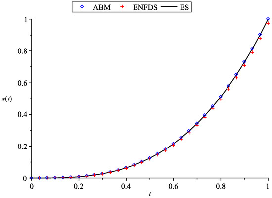
Figure 1. Numerical results using fractional Adams–Bashforth–Moulton (ABM) and explicit non-local finite-difference scheme (ENFDS) methods compared to exact solution (ES) for Example 1 at $N=30$.

Example 2.

In the Cauchy problem (9) we choose:

$$\omega \left(t\right)={\omega }_0^{\beta },f\left(t\right)=\frac{\mu t^{\delta }}{\mathsf{\Gamma }\left(1+\delta \right)},\lambda =0.$$

Then we come to the following problem:

$${\partial }_{0t}^{\beta }x\left(\tau \right)+{\omega }_0^{\beta }x\left(t\right)=\frac{\mu t^{\delta }}{\mathsf{\Gamma }\left(1+\delta \right)},x\left(0\right)={\alpha }_1,\dot{x}\left(0\right)={\alpha }_2.$$

(30)

The solution to the Cauchy problem (30) is the function:

$$x\left(t\right)={\alpha }_1{E}_{\beta ,1}\left(-{\left({\omega }_{0}t\right)}^{\beta }\right)+{\alpha }_{2}t{E}_{\beta ,2}\left(-{\left({\omega }_{0}t\right)}^{\beta }\right)+\mu t^{\beta +\delta }{E}_{\beta ,\beta +\delta +1}\left(-{\left({\omega }_{0}t\right)}^{\beta }\right),\delta >-\beta ,$$

(31)

where $E_{\alpha ,\beta }\left(z\right)={\displaystyle \sum _{k=0}^{\infty }}{\displaystyle \frac{z^k}{\mathsf{\Gamma }\left(\alpha k+\beta \right)}}$ is a Mittag–Leffler type function [5].

Let us consider numerical methods for solving the Cauchy problem (30) and compare them with the exact solution (31). First, consider the usual harmonic oscillator ($\beta =2$). We choose the values of the parameters in problem (30) as follows: $\delta =0.3,\mu =0.5,{\omega }_0=2,{\alpha }_1={\alpha }_2=1,t\in \left[0,1\right]$.

We see that the ABM method works in much the same way as the ENFDS method. The order of computational accuracy is shown in the following Table 4 and Table 5 (Figure 2 and Figure 3).

Table 4. Error analysis of numerical methods for Example 2 ($\beta =2$).

N	h	${\mathit{\xi }}_{\mathit{F}}$	${\mathit{\xi }}_{\mathit{PC}}$	${\mathit{p}}_{\mathit{F}}$	${\mathit{p}}_{\mathit{PC}}$
10	1/10	0.0962543446	0.0974594278	-	-
20	1/20	0.0483529972	0.0450644425	0.993246342	1.112812209
40	1/40	0.0243287977	0.0216596566	0.990940293	1.056979173
80	1/80	0.0122257234	0.0106471450	0.992745193	1.024543742
160	1/160	0.0061384979	0.0052867956	0.993962258	1.010001173
320	1/320	0.0030783418	0.0026378633	0.995732241	1.003023747
640	1/640	0.0015461838	0.0013190516	0.993441601	0.9998688

Table 5. Error analysis of numerical methods for Example 2 ($\beta =1.8$).

N	h	${\mathit{\xi }}_{\mathit{F}}$	${\mathit{\xi }}_{\mathit{PC}}$	${\mathit{p}}_{\mathit{F}}$	${\mathit{p}}_{\mathit{PC}}$
10	1/10	0.1220802888	0.0833919341	-	-
20	1/20	0.0632933442	0.0376498054	0.947704578	1.147265441
40	1/40	0.0326304379	0.0179210448	0.955835448	1.070987659
80	1/80	0.0167613673	0.0087578726	0.961078508	1.033002381
160	1/160	0.0085801061	0.0043373867	0.966072448	1.013754391
320	1/320	0.0043785606	0.0021615271	0.970538809	1.004775148
640	1/640	0.0022275871	0.0010803221	0.974974836	1.000589405

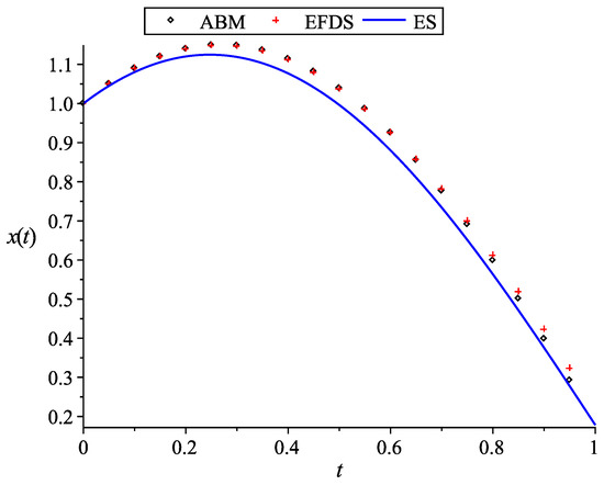
Figure 2. Numerical results using fractional Adams–Bashforth–Moulton (ABM) and explicit non-local finite-difference scheme (ENFDS) methods compared to exact solution (ES) for Example 2 at $N=20$ and $\beta =2$.

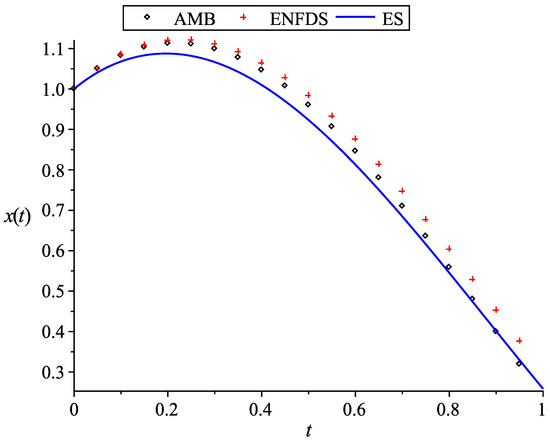
Figure 3. Numerical results using fractional Adams–Bashforth–Moulton (ABM) and explicit non-local finite-difference scheme (ENFDS) methods compared to exact solution (ES) for Example 2 at $N=20$ and $\beta =1.8$.

In the case $b=1.8$, the error analysis is given in Figure 3 and Table 5.

We see that the order of the computational accuracy of the methods tends to unity, i.e., the accuracy of the ABM method is similar to that of the ENFDS method, although the convergence rate is higher.

In this paper, we do not aim to improve the order of accuracy of numerical methods; this can be done, for example, by constructing an implicit non-local finite-difference scheme of a higher order of accuracy [14]. Since the ABM method converges faster than the ENFDS method, we will use it in the study of specific types of LFOs.

6. Forced Oscillations of Linear Fractional Oscillators

To determine the relationship of the orders of fractional derivatives in the model Equation (9) with the characteristics of the LFO, we will investigate their forced oscillations. In Equation (9), as the external force, we take a harmonic function with amplitude $\delta$ and frequency $\phi$: $f\left(t\right)=\delta cos\left(\phi t\right)$. Based on this, the model equation will take the form:

$${\partial }_{0t}^{\beta }x\left(\tau \right)+\lambda {\partial }_{0t}^{\gamma }x\left(\tau \right)+\omega \left(t\right)x\left(t\right)=\delta cos\left(\phi t\right),$$

(32)

Theorem 4.

Equation (32) is equivalent to the equation:

$$m\ddot{x}\left(t\right)+p\dot{x}\left(t\right)+s^{2}x\left(t\right)=\delta cos\left(\phi t\right),$$

(33)

where $m=-{\phi }^{\beta -2}cos\left(\beta \pi /\phantom{\beta \pi 2}2\right),p={\phi }^{\beta -1}sin\left(\beta \pi /\phantom{\beta \pi 2}2\right)+\lambda {\phi }^{\gamma -1}sin\left(\gamma \pi /\phantom{\gamma \pi 2}2\right)$, $s^2=\omega \left(t\right)+\lambda {\phi }^{\gamma }cos\left(\gamma \pi /\phantom{\gamma \pi 2}2\right)$, $x\left(t\right)=Acos\left(u\right),\dot{x}\left(t\right)=-A\phi sin\left(u\right),\ddot{x}\left(t\right)=-A{\phi }^{2}cos\left(u\right),u=\phi t+\mathsf{\Phi }$, $A,\mathsf{\Phi }$ is the amplitude and phase of steady-state oscillations.

Proof. 

We will seek a solution to Equation (32) in the form:

$$x\left(t\right)=Acos\left(\phi t+\mathsf{\Phi }\right)=Acos\left(u\right),$$

(34)

Taking into account (2), Equation (32) can be rewritten as:

$$\frac{1}{\mathsf{\Gamma }\left(2-\beta \right)}\underset{0}{\overset{t}{\int }}\frac{\ddot{x}\left(\tau \right)d\tau }{{\left(t-\tau \right)}^{\beta -1}}+\frac{\lambda }{\mathsf{\Gamma }\left(1-\gamma \right)}\underset{0}{\overset{t}{\int }}\frac{\dot{x}\left(\tau \right)d\tau }{{\left(t-\tau \right)}^{\gamma }}+\omega \left(t\right)x\left(t\right)=\delta cos\left(\phi t\right).$$

(35)

Then the first term in (35), taking into account representation (34), can be represented as:

$$\frac{1}{\mathsf{\Gamma }\left(2-\beta \right)}\underset{0}{\overset{t}{\int }}\frac{\ddot{x}\left(\tau \right)d\tau }{{\left(t-\tau \right)}^{\beta -1}}\frac{1}{\mathsf{\Gamma }\left(2-\beta \right)}\underset{0}{\overset{t}{\int }}{v}^{1-\beta }\ddot{x}\left(t-v\right)dv=-\frac{A{\phi }^2}{\mathsf{\Gamma }\left(2-\beta \right)}\underset{0}{\overset{t}{\int }}{v}^{1-\beta }cos\left(\phi \left(t-v\right)+\mathsf{\Phi }\right)dv$$

$$=-\frac{A{\phi }^2}{\mathsf{\Gamma }\left(2-\beta \right)}\underset{0}{\overset{t}{\int }}{v}^{1-\beta }\left[cos\left(\phi \left(t-v\right)\right)cos\left(\mathsf{\Phi }\right)-sin\left(\phi \left(t-v\right)\right)sin\left(\mathsf{\Phi }\right)\right]dv$$

$$=-\frac{A{\phi }^{2}cos\left(\mathsf{\Phi }\right)}{\mathsf{\Gamma }\left(2-\beta \right)}\underset{0}{\overset{t}{\int }}{v}^{1-\beta }cos\left(\phi \left(t-v\right)\right)dv+\frac{A{\phi }^{2}sin\left(\mathsf{\Phi }\right)}{\mathsf{\Gamma }\left(2-\beta \right)}\underset{0}{\overset{t}{\int }}{v}^{1-\beta }sin\left(\phi \left(t-v\right)\right)dv$$

$$=-\frac{A{\phi }^{2}cos\left(\mathsf{\Phi }\right)}{\mathsf{\Gamma }\left(2-\beta \right)}\underset{0}{\overset{t}{\int }}{v}^{1-\beta }\left[cos\left(\phi t\right)cos\left(\phi v\right)+sin\left(\phi t\right)sin\left(\phi v\right)\right]dv$$

$$+\frac{A{\phi }^{2}sin\left(\mathsf{\Phi }\right)}{\mathsf{\Gamma }\left(2-\beta \right)}\underset{0}{\overset{t}{\int }}{v}^{1-\beta }\left[sin\left(\phi t\right)cos\left(\phi v\right)-cos\left(\phi t\right)sin\left(\phi v\right)\right]dv$$

$$=-\frac{A{\phi }^{2}cos\left(\mathsf{\Phi }\right)cos\left(\phi t\right)}{\mathsf{\Gamma }\left(2-\beta \right)}\underset{0}{\overset{t}{\int }}{v}^{1-\beta }cos\left(\phi v\right)dv-\frac{A{\phi }^{2}cos\left(\mathsf{\Phi }\right)sin\left(\phi t\right)}{\mathsf{\Gamma }\left(2-\beta \right)}\underset{0}{\overset{t}{\int }}{v}^{1-\beta }sin\left(\phi v\right)dv$$

(36)

$$+\frac{A{\phi }^{2}sin\left(\mathsf{\Phi }\right)sin\left(\phi t\right)}{\mathsf{\Gamma }\left(2-\beta \right)}\underset{0}{\overset{t}{\int }}{v}^{1-\beta }cos\left(\phi v\right)dv-\frac{A{\phi }^{2}sin\left(\mathsf{\Phi }\right)cos\left(\omega t\right)}{\mathsf{\Gamma }\left(2-\beta \right)}\underset{0}{\overset{t}{\int }}{v}^{1-\beta }sin\left(\phi v\right)dv$$

$$=\left[sin\left(\mathsf{\Phi }\right)sin\left(\phi t\right)-cos\left(\mathsf{\Phi }\right)cos\left(\phi t\right)\right]\frac{A{\phi }^2}{\mathsf{\Gamma }\left(2-\beta \right)}\underset{0}{\overset{t}{\int }}{v}^{1-\beta }cos\left(\phi v\right)dv$$

$$-\left[sin\left(\mathsf{\Phi }\right)cos\left(\phi t\right)+cos\left(\mathsf{\Phi }\right)sin\left(\phi t\right)\right]\frac{A{\phi }^2}{\mathsf{\Gamma }\left(2-\beta \right)}\underset{0}{\overset{t}{\int }}{v}^{1-\beta }sin\left(\phi v\right)dv$$

$$=\frac{-A{\phi }^{2}cos\left(u\right)}{\mathsf{\Gamma }\left(2-\beta \right)}\underset{0}{\overset{t}{\int }}{v}^{1-\beta }cos\left(\phi v\right)dv-\frac{A{\phi }^{2}sin\left(u\right)}{\mathsf{\Gamma }\left(2-\beta \right)}\underset{0}{\overset{t}{\int }}{v}^{1-\beta }sin\left(\phi v\right)dv.$$

In the case of steady-state oscillations at $t\to \infty$, the integrals in (36) can be written as follows [5]:

$$\underset{0}{\overset{t}{\int }}{v}^{1-\beta }cos\left(\phi v\right)dv\approx \frac{\mathsf{\Gamma }\left(2-\beta \right)}{{\phi }^{2-\beta }}sin\left(\left(\beta -1\right)\pi /\phantom{\left(\beta -1\right)\pi 2}2\right)=-\frac{\mathsf{\Gamma }\left(2-\beta \right)}{{\phi }^{2-\beta }}cos\left(\beta \pi /\phantom{\beta \pi 2}2\right).$$

(37)

$$\underset{0}{\overset{t}{\int }}{v}^{1-\beta }sin\left(\phi v\right)dv\approx \frac{\mathsf{\Gamma }\left(2-\beta \right)}{{\phi }^{2-\beta }}cos\left(\left(\beta -1\right)\pi /\phantom{\left(\beta -1\right)\pi 2}2\right)=\frac{\mathsf{\Gamma }\left(2-\beta \right)}{{\phi }^{2-\beta }}sin\left(\beta \pi /\phantom{\beta \pi 2}2\right).$$

(38)

Taking into account relations (37) and (38), we get:

$$\frac{1}{\mathsf{\Gamma }\left(2-\beta \right)}\underset{0}{\overset{t}{\int }}\frac{\ddot{x}\left(\tau \right)d\tau }{{\left(t-\tau \right)}^{\beta -1}}=A{\phi }^{\beta }\left(cos\left(u\right)cos\left(\beta \pi /\phantom{\beta \pi 2}2\right)-sin\left(u\right)sin\left(\beta \pi /\phantom{\beta \pi 2}2\right)\right).$$

(39)

Similarly, the second term in (35) will have the form:

$$\frac{\lambda }{\mathsf{\Gamma }\left(1-\gamma \right)}\underset{0}{\overset{t}{\int }}\frac{\dot{x}\left(\tau \right)d\tau }{{\left(t-\tau \right)}^{\gamma }}=\lambda A{\phi }^{\gamma }\left(cos\left(\gamma \pi /\phantom{\gamma \pi 2}2\right)cos\left(u\right)-sin\left(\gamma \pi /\phantom{\gamma \pi 2}2\right)sin\left(u\right)\right).$$

(40)

Taking into account (34), (38) and (40), Equation (32) can be rewritten as:

$$A{\phi }^{\beta }\left(cos\left(u\right)cos\left(\beta \pi /\phantom{\beta \pi 2}2\right)-sin\left(u\right)sin\left(\beta \pi /\phantom{\beta \pi 2}2\right)\right)+\lambda A{\phi }^{\gamma }\left(cos\left(\gamma \pi /\phantom{\gamma \pi 2}2\right)cos\left(u\right)-sin\left(\gamma \pi /\phantom{\gamma \pi 2}2\right)sin\left(u\right)\right)$$

$$+\omega \left(t\right)Acos\left(u\right)=\delta cos\left(\phi t\right).$$

(41)

Taking into account in Equation (33) that $\dot{x}\left(t\right)=-A\phi sin\left(u\right),\ddot{x}\left(t\right)=-A{\phi }^{2}cos\left(u\right)$, we arrive at Equation (33). ☐

Remark 6.

Please note that Equation (33) is a classical linear oscillator with friction and external harmonic action, for which the relations for the amplitude–frequency (AFC), phase-frequency (PFC) characteristics and Q-factor are known:

$$A=\frac{\delta }{\sqrt{U^2+W^2}},\mathsf{\Phi }=arctan\left(-\frac{W}{U}\right),Q={\displaystyle \frac{s}{p}},$$

(42)

where $U=s^2-{\phi }^{2}m,W=\phi p$.

Formulas (42) for the AFC and PFC can be rewritten as follows:

$$A=\frac{\delta }{\sqrt{{\phi }^{2\beta }+{\omega }^2\left(t\right)+\lambda {\phi }^{\gamma }\left(\lambda {\phi }^{\gamma }+2{\phi }^{\gamma }cos\left(\left(\beta -\gamma \right)\pi /\phantom{\left(\beta -\gamma \right)\pi 2}2\right)+2\omega \left(t\right)cos\left(\gamma \pi /\phantom{\gamma \pi 2}2\right)\right)+2\omega \left(t\right){\phi }^{\beta }cos\left(\beta \pi /\phantom{\beta \pi 2}2\right)}},$$

(43)

$$\mathsf{\Phi }=arctan\left(-\frac{\left({\phi }^{\beta }sin\left(\beta \pi /\phantom{\beta \pi 2}2\right)+\lambda {\phi }^{\gamma }sin\left(\gamma \pi /\phantom{\gamma \pi 2}2\right)\right)}{\omega \left(t\right)+\lambda {\phi }^{\gamma }cos\left(\gamma \pi /\phantom{\gamma \pi 2}2\right)+{\phi }^{\beta }cos\left(\beta \pi /\phantom{\beta \pi 2}2\right)}\right),$$

$$Q={\displaystyle \frac{\sqrt{\omega \left(t\right)+\lambda {\phi }^{\gamma }cos\left(\gamma \pi /2\right)}}{{\phi }^{\beta -1}sin\left(\beta \pi /2\right)+\lambda {\phi }^{\gamma -1}sin\left(\gamma \pi /2\right)}}.$$

Remark 7.

Recall that the AFC determines the dependence of the amplitude of steady-state oscillations on the frequency of the harmonic input signal. The maximum value of the amplitude corresponds to the value of the resonant frequency. Therefore, the AFC curves are also called resonant. PFC is the dependence of the phase difference between the input and output signals on the frequency of the harmonic input signal. Q-factor is a parameter of an oscillatory system that determines the width of the resonance and characterizes how many times the energy reserves in the system are greater than the energy losses during the phase change by 1 radian.

Figure 4 shows the resonance curves AFC obtained by formula (43), as well as using the ABM method, taking into account the parameter values [18]: $\lambda =0.5,\delta =50,\gamma =1,\omega \left(t\right)={\omega }_0=1$.

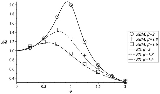
Figure 4. Resonance curves plotted for different values of the parameter $\beta$ by Formula (43) and by the ABM method.

Figure 4 shows that in the classical case with the value of the parameter $\beta =2$, the maximum amplitude is achieved at the value of the frequency $\varphi =1$, i.e., resonance occurs ($\varphi ={\omega }_0=1$). Furthermore, with decreasing parameter $\beta$, the maximum amplitude decreases, and the resonant frequency shifts to the region of lower frequencies. Therefore, it can be concluded that the parameter $\beta$ is responsible for the intensity of energy dissipation in an oscillatory system with memory.

From Figure 4, we also see that the resonance curves obtained by the numerical ABM algorithm give an acceptable result. The numerical algorithm for calculating the resonance curves is based on the fact that over time the amplitude of the oscillations reaches a steady state. Therefore, we first calculate the initial LFO model using the ABM method for sufficiently large t and different values of the frequency of external influence $\phi$.

Figure 5 shows the curves of the phase-frequency characteristic $\mathsf{\Phi }$ at different values of the parameters $\beta$ and $\gamma$.

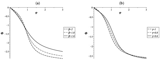
Figure 5. PFC curves plotted for different values of $\beta$ and a fixed value of $\gamma =1$ (a) and for different values of gamma and a fixed value of $\beta =1.8$ (b).

From Figure 5a, for the classical case at $\beta =2$ and $\gamma =1$, the limiting value of the phase shift at $\phi \to \infty$ is $\mathsf{\Phi }=-\pi$. With a decrease in the values of the parameter $\beta$, the limiting phase shift will be $\mathsf{\Phi }=-\beta \pi /2$, i.e., will decrease. Please note that the PFC curves are rearranged in reverse order, which is typical for memory effects.

Figure 5b shows PFC curves plotted at various values of the parameter $\gamma$. It can be noted that in this case the limiting value of the phase shift remains practically unchanged, but the regrouping of the curves remains.

Figure 6a shows the Q-factor plotted for various values of beta and fixed frequency $\phi =0.5,1,1.5$, as well as $\gamma =1$. It is seen that with decreasing values of the parameter $\beta$, the Q-factor decreases for each fixed value of the frequency $\phi$. This fact confirms that the beta parameter is responsible for the intensity of the LFO energy dissipation.

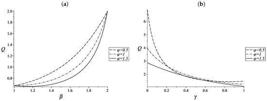
Figure 6. Calculated Q-factor curves plotted depending on the values of the parameters $\beta$ (a) and $\gamma$ (b).

Figure 6b shows the Q-factor obtained for different values of the parameter gamma and fixed values of the frequency $\phi =0.5,1,1.5$, as well as $\beta =1.8$. Here we can see that the Q-factor increases with decreasing gamma parameter values. Therefore, the $\gamma$ parameter, as well as the beta parameter, is responsible for the intensity of energy dissipation. Please note that the $\beta$ and $\gamma$ parameters act in different directions, i.e., if the $\beta$ parameter decreases the Q-factor, then the $\gamma$ parameter, on the contrary, leads to its increase.

In the previous examples in Formula (43), we chose the natural frequency $\omega \left(t\right)$ as a constant. Consider more general cases when $\omega \left(t\right)=t$ and $\omega \left(t\right)=1+3cos\left(2t\right)$. The first case corresponds to the fractional Airy oscillator, and the second to the fractional Mathieu oscillator. We will explore them in more detail in the next section.

Figure 7 shows AFC surfaces and Q-factor surfaces plotted against $\beta$ and t for a fractional Airy oscillator. Here the parameter values were chosen: gray—$\gamma =0.8$, blue—$\gamma =0.6$, red—$\gamma =0.4$, $\phi =0.5$, the rest of the parameter values are taken from the previous example.

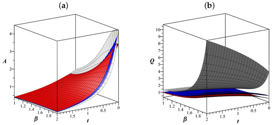
Figure 7. AFC surfaces (a) and Q-factor surfaces (b) plotted against $\beta$ and t.

In Figure 7a, we can see that as the values of the $\beta$ parameter decrease over the entire time interval [0,2], AFC also decreases for each value of $\gamma$. Figure 7b confirms this pattern. We see that the Q-factor decreases with decreasing values of the $\beta$ parameter for each value of $\gamma$ over the entire time interval.

Figure 8 shows the surfaces of the frequency response and Q-factor of a fractional Airy oscillator depending on $\gamma$ and t. Here the values of the $\beta$ parameter were chosen: 1.8—gray, 1.6—blue, 1.4—red. Leave the rest of the parameters unchanged.

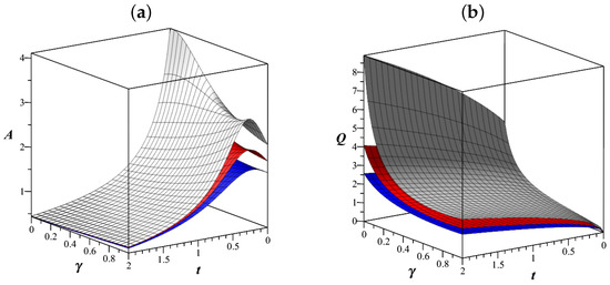
Figure 8. AFC surfaces (a) and Q-factor surfaces (b) plotted against $\gamma$ and t.

In Figure 8a,b, we see that the AFC and Q-factor decrease with decreasing $\gamma$ values for various fixed $\beta$ values over the entire time interval of t.

Figure 9 and Figure 10, by analogy with Figure 7 and Figure 8, show the AFC and Q-factor surfaces for the Mathieu fractional oscillator at different values of the parameters $\beta$ and $\gamma$.

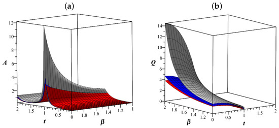
Figure 9. AFC surfaces (a) and Q-factor surfaces (b) plotted against $\gamma$ and t.

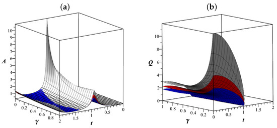
Figure 10. AFC surfaces (a) and Q-factor surfaces (b) plotted against $\beta$ and t.

Figure 9 and Figure 10 confirm the conclusions drawn earlier: the parameters $\beta$ and $\gamma$ are responsible for the intensity of energy dissipation and act in different directions. With a decrease in the parameter $\beta$, the intensity of energy dissipation increases, and with a decrease in the parameter $\gamma$, the intensity of energy dissipation decreases.

7. Research of Some Types of LFO

7.1. An Analogue of a Harmonic Oscillator

Consider an analogue of a harmonic oscillator (AHO), which is specified by the following parameters in the Cauchy problem (9): $\omega \left(t\right)={\omega }_0^{\beta }$, $f\left(t\right)=\delta cos\left(\phi t\right)$, where $\delta$, $\phi$ are the amplitude and frequency of the external harmonic influence. We get the following Cauchy problem:

$${\partial }_{0t}^{\beta }x\left(\tau \right)+\lambda {\partial }_{0t}^{\gamma }x\left(\tau \right)+{\omega }_0^{\beta }x\left(t\right)=\delta cos\left(\phi t\right),x\left(0\right)={\alpha }_1,\dot{x}\left(0\right)={\alpha }_2,$$

(44)

Please note that the Cauchy problem (44) with the values of the parameters $\beta =1$, $\gamma =1$ will describe a linear harmonic oscillator.

Let us investigate the problem (44) by the ABM method under conditions of free oscillations ($\delta =0$) both without friction ($\lambda =0$) and with its presence ($\lambda \ne 0$) for a harmonic oscillator. The remaining values of the parameters of problem (44) are chosen as follows: $t\in \left[0,20\right],{\omega }_0^2=1,\lambda =0.3,x\left(0\right)=0.2,\dot{x}\left(0\right)=0.1$. For the ABM method, let us choose $N=2000$ points of the computational grid. The results of the numerical study are shown in Figure 11.

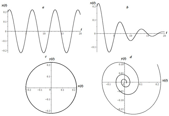
Figure 11. Harmonic oscillator ($\beta =2,\gamma =1$) without friction: (a)—oscillogram and (c)—phase trajectory, as well as with friction: (b)—oscillogram and (d)—phase trajectory, in conditions of free oscillations.

In Figure 11, we see typical calculated curves of oscillograms and phase trajectories of a harmonic oscillator under free oscillation conditions. In the absence of friction, the oscillogram (Figure 11a) has a constant oscillation amplitude, and its corresponding phase trajectory (Figure 11c) is a closed line, the rest point of the oscillator in this case is the center. In the case of damping, the oscillatory mode has a damping nature (Figure 11b), the phase trajectory is open (Figure 11d), the rest point is a stable focus.

Consider an AHO without friction, taking into account free vibrations. Let the fractional force of inertia be of order $\beta =1.8$, and the values of the remaining parameters are taken from the previous case. The calculation results are shown in Figure 12.

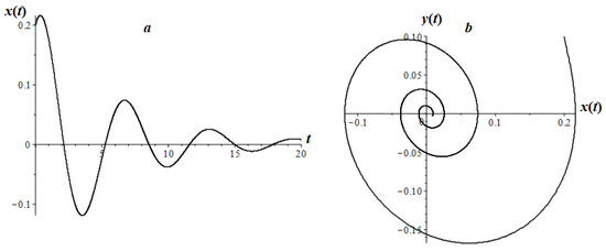
Figure 12. AHO, experiencing free oscillations without damping at $\beta =1.8$: (a) oscillogram; (b) phase trajectory.

Figure 12 shows that the introduction of a fractional derivative to describe the inertial force results in a damped oscillatory mode, similar to the damped harmonic oscillator mode (Figure 3b,c). This is in good agreement with V. Volterra’s hereditary theory.

Let us consider the resonance effect for a harmonic oscillator—an increase in the oscillation amplitude when the frequency of free oscillations and the frequency of an external periodic action (${\omega }_0^2=\phi =1$) without friction coincide. We choose the amplitude of the external periodic action $\delta =2$ and $t\in \left[0.60\right]$.

Figure 13 shows the classical resonance for a frictionless harmonic oscillator. The oscillogram (Figure 13a) has an infinitely increasing amplitude, and the phase trajectory (Figure 13b) has the form of an unwinding spiral (resting point is an unstable focus).

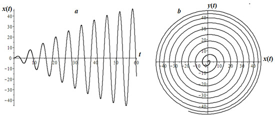
Figure 13. Harmonic oscillator without friction in resonance mode: (a) oscillogram; (b) phase trajectory.

The case of AHO without friction with ${\omega }_0^{1.8}=\phi =1$, for example, with the parameter $\beta =1.8$, is shown in Figure 14.

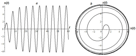
Figure 14. AHO without friction at $\beta =1.8$ and ${\omega }_0^{1.8}=\phi =1$.

In this case, we do not observe the resonance effect, due to the fact that the natural oscillations of the oscillator have a damping character, and due to an external harmonic effect, over time, the amplitude of the oscillations reaches a steady state (Figure 14a). The phase trajectory over time “winds” on a closed trajectory and reaches the limit cycle (Figure 14b).

It should be noted that with a decrease in the value of the parameter, for example, $\beta =1.6$, the phase trajectory reaches the limit cycle faster (Figure 15b), due to the rapid damping of natural oscillations (Figure 15a).

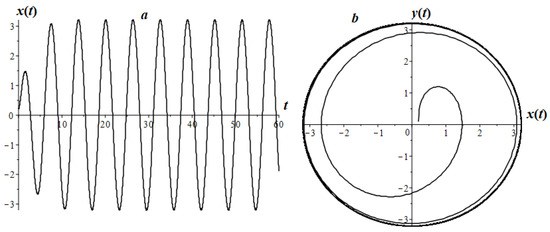
Figure 15. AHO without friction at $\beta =1.8$ and ${\omega }_0^{1.6}=\varphi =1$.

7.2. Fractional Oscillator Mathieu

The Mathieu oscillator is of wide interest, since it has a parametric resonance, which arises as a result of changes in the parameters ${\xi }_1$ and ${\xi }_2$, which is associated with the instability of the oscillatory system, at which the amplitude of oscillations increases. For the first time, this oscillator was investigated by E. Mathieu in 1868 in the problem of oscillation of a membrane with an elliptical boundary [19].

The Cauchy problem (9) for the fractional Mathieu oscillator when choosing the functions: $\omega \left(t\right)={\xi }_1+{\xi }_{2}cos\left(\omega t\right)$, where ${\xi }_1$, ${\xi }_2$ are positive parameters that determine the parametric resonance, has the form:

$${\partial }_{0t}^{\beta }x\left(\tau \right)+\lambda {\partial }_{0t}^{\gamma }x\left(\tau \right)+\left({\xi }_1+{\xi }_{2}cos\left(\omega t\right)\right)x\left(t\right)=\delta cos\left(\phi t\right),x\left(0\right)={\alpha }_1,\dot{x}\left(0\right)={\alpha }_2,$$

(45)

In the case when $\beta =2$, $\gamma =1$, the Cauchy problem (45) turns into the classical problem for parametric resonance. Let us consider this case under conditions of free oscillations $\delta =0$ and without friction $\lambda =0$. To do this, we determine the values of the following parameters: ${\xi }_1=2,{\xi }_2={\omega }_0=1,x\left(0\right)=0.2,\dot{x}\left(0\right)=0.1,t\in \left[0,100\right]$, for the computational grid of the ABM method, we choose $N=2000$. The calculation results are shown in Figure 16.

Figure 16. Ordinary Mathieu oscillator without friction in free oscillation mode: (a) oscillogram; (b) phase trajectory.

In Figure 16, we see the classic effect of parametric resonance, when resonance occurs as a result of changing the parameters ${\xi }_1$ and ${\xi }_2$. In order to investigate the effect of parametric resonance, the Strett–Ains diagrams are constructed, which determine the boundaries of the instability region in which it exists [20,21]. As a result of generalization to the fractional case, the Strett–Ains diagrams depend on the values of the parameters beta and gamma [22]. Let us choose the parameter $\beta =1.9$, and leave the rest unchanged. The calculation result is shown in Figure 17.

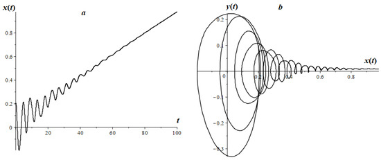
Figure 17. Aperiodic mode of the Mathieu fractional oscillator with no friction in the free oscillation mode: (a) oscillogram; (b) phase trajectory.

In Figure 17a, we see damped oscillations on the one hand, and on the other, an aperiodic regime, which characterizes the growing dynamics, so there is no parametric resonance here. Let us take the values of the parameters from [22]: ${\xi }_1=0.25,{\xi }_2=0.5,\beta =1.8$, which correspond to falling into the region of instability—the existence of the main resonance. We leave the rest of the parameters from the previous case.

In Figure 18, we see a significant increase in the amplitude of oscillations (Figure 18a, and the phase trajectory unwinds in Figure 18b. Taking into account fractional friction ($\lambda =0.3,\gamma =0.8$), we will get a damped vibration mode (Figure 19).

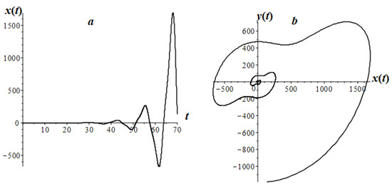
Figure 18. Parametric resonance of the Mathieu fractional oscillator at $\beta =1.8$: (a) oscillogram; (b) phase trajectory.

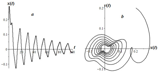
Figure 19. Damped mode of the Mathieu fractional oscillator: (a) oscillogram; (b) phase trajectory.

In the presence of an external influence, the Mathieu fractional oscillator can have rather complex, multi-periodic oscillatory modes. Let’s take the parameter case as an example: ${\xi }_1=3,{\xi }_2=5,\beta =1.6,\gamma =0.8,\lambda =0.9,\delta =\phi =3,t\in \left[0,100\right]$. The simulation results are shown in Figure 20.

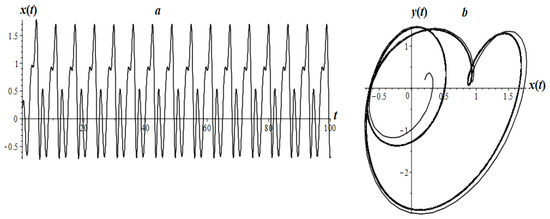
Figure 20. Multi-periodic Fractional Mathieu Oscillator Mode: (a) oscillogram; (b) phase trajectory.

7.3. Airy Fractional Oscillator

The Airy oscillator is an oscillation model that was first investigated by British astronomer George Airy in optics to describe the appearance of stars as a point source of light in a telescope [23]. Airy oscillations are also considered within the framework of the theory of diffractive optics for obtaining laser beams [24].

Cauchy problem (9) for the fractional Airy oscillator when choosing the functions $\omega \left(t\right)=t,f\left(t\right)=\delta cos\left(\phi t\right)$:

$${\partial }_{0t}^{\beta }x\left(\tau \right)+\lambda {\partial }_{0t}^{\gamma }x\left(\tau \right)+tx\left(t\right)=\delta cos\left(\phi t\right),x\left(0\right)={\alpha }_1,\dot{x}\left(0\right)={\alpha }_2,$$

(46)

In the case $\beta =2,\gamma =1$, the Cauchy problem (46) turns into the Cauchy problem for the classical Airy oscillator (Figure 21).

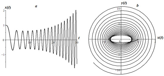
Figure 21. The classic Airy oscillator: (a) oscillogram; (b) phase trajectory.

Figure 21 shows the calculated oscillogram (Figure 21a) and the phase trajectory (Figure 22b) with the following parameter values: $\lambda =\delta =0,t\in \left[0,30\right],x\left(0\right)=1,\dot{x}\left(0\right)=0$, and for the calculation grid the number of nodes is $N=4000$. It is known that the classical Airy oscillator has an oscillatory regime with continuous amplitude [24].

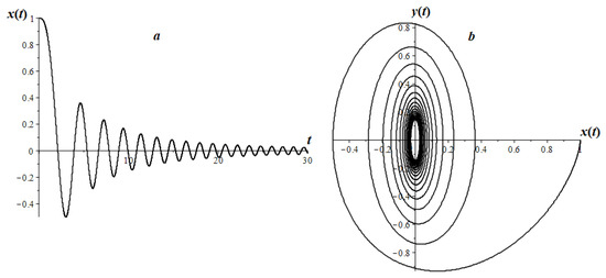
Figure 22. The classic Airy oscillator with friction: (a) oscillogram; (b) phase trajectory.

In the presence of friction $\lambda =0.3$, the Airy oscillations reach the steady state (Figure 22a), and the phase trajectory (Figure 22b) enters a constant orbit—the limit cycle.

In the case of a fractional Airy oscillator at $\beta =1.8$ without damping ($\lambda =0$) and external influence ($\delta =0$), we will get a damped oscillatory mode (Figure 23).

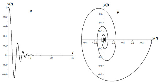
Figure 23. Damped oscillatory mode of the fractional Airy oscillator: (a) oscillogram; (b) phase trajectory.

The case of taking into account external influence and friction is shown in Figure 24.

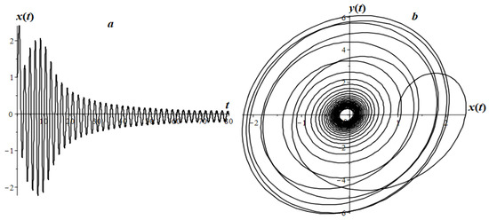
Figure 24. Fractional Airy oscillator with friction and external action: (a) oscillogram; (b) phase trajectory.

Here, in Figure 24a, we see that the growth of the amplitude at the beginning of the oscillatory process is replaced by its decline, and then an exit to the steady state occurs. The phase trajectory reaches the limit cycle (Figure 1b).

8. Discussion

The article considered a wide class of linear fractional oscillators in the case when the memory function was chosen as a power-law one (4). However, the memory function can be chosen differently, based on the conditions of the problem or experimental data. Therefore, the class of hereditary oscillators is much wider and richer than the class of fractional oscillators. On the other hand, the definition of the memory function can give a new definition of the derivative of fractional order, which will make it possible to develop fractional calculus in the future.

In this work, several numerical methods for solving the Cauchy problem were chosen: ABM and ENFD, which were implemented in the Maple computer environment. We did not set ourselves the task of improving the accuracy of these methods, therefore, it is possible to use other more accurate methods.

It is of interest to study the asymptotic stability of the equilibrium points of the fractional dynamical system (9).

Also of interest is the study of LFO with variable memory. In this case, derivatives of fractional variable orders appear in the model equation of the Cauchy problem (9). Some aspects of the numerical analysis of the generalized Cauchy problem (9) were considered by the author in [25].

In developing the research topic, it is of particular interest to consider the Cauchy problem (9) in terms of the fractional Riemann–Liouville derivative with non-local initial conditions [26,27].

9. Conclusions

In this paper, a numerical analysis of the Cauchy problem for a model class of fractional linear oscillators was carried out. The ENFDS and ABM methods were considered to be numerical methods. It was shown on test examples that the ABM method converges faster and is more accurate (not always) than the ENFDS method. Forced oscillations of the LFO are investigated. The amplitude–frequency and phase-frequency characteristics, as well as the Q-factor, have been investigated. It is shown that the parameters $\beta$ and $\gamma$ are responsible for the intensity of the LFO energy dissipation, which is very important for engineering applications. Using the ABM method, the calculated curves of oscillograms and phase trajectories of some LFO: Mathieu, Airy, and AHO were constructed and their properties were investigated. The results obtained earlier are confirmed.

References

- Andronov, A.; Vitt, A.; Khaikin, S. Theory of Oscillators: Adiwes International Series in Physics; Elsevier: Amsterdam, The Netherlands, 2013; Volume 4, p. 848. [Google Scholar]
- Danylchuk, H.; Kibalnyk, L.; Serdiuk, O. Study of critical phenomena in economic systems using a model of damped oscillations. SHS Web Conf. 2019, 65, 06008. [Google Scholar] [CrossRef]
- Li, Z.; Yang, Q. Systems and synthetic biology approaches in understanding biological oscillators. Quant Biol. 2018, 6, 1–14. [Google Scholar] [CrossRef] [PubMed]
- Volterra, V. Sur les equations integro-differentielles et leurs applications. Acta Math. 1912, 35, 295–356. [Google Scholar] [CrossRef]
- Kilbas, A.; Srivastava, H.; Trujillo, J. Theory and Applications of Fractional Differential Equations; Elsevier: Amsterdam, The Netherlands, 2006; Volume 204, p. 523. [Google Scholar]
- Oldham, K.; Spanier, J. The Fractional Calculus. Theory and Applications of Differentiation and Integration to Arbitrary Order; Academic Press: London, UK, 1974; p. 240. [Google Scholar]
- Miller, K.; Ross, B. An Introduction to the Fractional Calculus and Fractional Differntial Equations; A Wiley-Interscience Publication: New York, NY, USA, 1993; p. 384. [Google Scholar]
- Pskhu, A.; Rekhviashvili, S. Analysis of Forced Oscillations of a Fractional Oscillator. Tech. Phys. Lett. 2018, 44, 1218–1221. [Google Scholar] [CrossRef]
- Parovik, R. Amplitude-Frequency and Phase-Frequency Perfomances of Forced Oscillations of a Nonlinear Fractional Oscillator. Tech. Phys. Lett. 2019, 45, 660–663. [Google Scholar] [CrossRef]
- Khalouta, A.; Kadem, A. A New Method to Solve Fractional Differential Equations: Inverse Fractional Shehu Transform Method. Appl. Appl. Math. 2019, 14, 926–941. [Google Scholar]
- Momani, S.; Odibat, Z. Numerical comparison of methods for solving linear differential equations of fractional order. Chaos Solitons Fractals 2007, 31, 1248–1255. [Google Scholar] [CrossRef]
- Diethelm, K.; Ford, N.; Freed, A.; Luchko, Y. Algorithms for the fractional calculus: A selection of numerical methods. Comput. Methods Appl. Mech. Eng. 2005, 194, 743–773. [Google Scholar] [CrossRef]
- Parovik, R. Mathematical model of a wide class memory oscillators. Bull. South Ural State Univ. Ser. Math. Model. Program. 2018, 11, 108–122. [Google Scholar] [CrossRef]
- Garrappa, R. Numerical Solution of Fractional Differential Equations: A Survey and a Software Tutorial. Mathematics 2018, 6, 16. [Google Scholar] [CrossRef]
- Yang, C.; Liu, F. A computationally effective predictor-corrector method for simulating fractional-order dynamical control system. ANZIAM J. 2006, 47, 168–184. [Google Scholar] [CrossRef]
- Diethelm, K.; Ford, N.; Freed, A. A predictor-corrector approach for the numerical solution of fractional differential equations. Nonlinear Dyn. 2002, 29, 3–22. [Google Scholar] [CrossRef]
- Rekhviashvili, S.; Pskhu, A.; Agarwal, P.; Jain, S. Application of the fractional oscillator model to describe damped vibrations. Turk. J. Phys. 2019, 43, 236–242. [Google Scholar] [CrossRef]
- Parovik, R. Quality Factor of Forced Oscillations of a Linear Fractional Oscillator. Tech. Phys. 2020, 65, 1015–1019. [Google Scholar] [CrossRef]
- Mathieu, E. Mémoire sur le mouvement vibratoire d’une membrane de forme elliptique. J. Math. Pures Appl. 1868, 13, 137–203. [Google Scholar]
- Butikov, I. Analytical expressions for stability regions in the Ince–Strutt diagram of Mathieu equation. Am. J. Phys. 2018, 86, 257–267. [Google Scholar] [CrossRef]
- Rand, R.; Sah, S.; Suchorsky, M. Fractional Mathieu equation. Commun. Nonlinear Sci. Numer. Simul. 2010, 15, 3254–3262. [Google Scholar] [CrossRef]
- Parovik, R. Fractal parametric oscillator as a model of a nonlinear oscillation system in natural mediums. Int. J. Commun. Netw. Syst. Sci. 2013, 6, 134–138. [Google Scholar] [CrossRef]
- Airy, G. On the intensity of light in the neighbourhood of a caustic. Trans. Camb. Philos. Soc. 1838, 6, 379–402. [Google Scholar]
- Siviloglou, G. Accelerating finite energy Airy beams. Opt. Lett. 2007, 32, 979–981. [Google Scholar] [CrossRef]
- Parovik, R. Explicit finite-difference scheme for the numerical solution of the model equation of nonlinear hereditary oscillator with variable-order fractional derivatives. Arch. Control Sci. 2016, 26, 429–435. [Google Scholar] [CrossRef]
- Zhang, X.G.; Liu, L.S.; Wu, Y.H. Multiple positive solutions of a singular fractional differential equation with negatively perturbed term. Math. Comput. Model. 2012, 55, 1263–1274. [Google Scholar] [CrossRef]
- Zhang, X.G.; Wu, Y.H.; Caccetta, L. Nonlocal fractional order differential equations with changing-sign singular perturbation. Appl. Math. Model. 2015, 39, 6543–6552. [Google Scholar] [CrossRef]
Publisher’s Note: MDPI stays neutral with regard to jurisdictional claims in published maps and institutional affiliations. |
© 2020 by the author. Licensee MDPI, Basel, Switzerland. This article is an open access article distributed under the terms and conditions of the Creative Commons Attribution (CC BY) license (http://creativecommons.org/licenses/by/4.0/).