Abstract
Improving the efficiency of solar panels is the main task of solar energy generation. One of the methods is a solar tracking system. One of the most important parameters of tracking systems is a precise orientation to the Sun. In this paper, the performance of single-axis solar trackers based on schedule and light dependent resistor (LDR) photosensors, as well as a stationary photovoltaic installation in various weather conditions, were compared. A comparative analysis of the operation of a manufactured schedule solar tracker and an LDR solar tracker in different weather conditions was performed; in addition, a simple method for determining the rotation angle of a solar tracker based on the encoder was proposed. Finally, the performance of the manufactured solar trackers was calculated, taking into account various weather conditions for one year. The proposed single-axis solar tracker based on schedule showed better results in cloudy and rainy weather conditions. The obtained results can be used for designing solar trackers in areas with a variable climate.
1. Introduction
The development of solar energy conversion methods inevitably lead to the development of autonomous systems based on photovoltaic panels, such as portable and low-power solar power plants, street lighting systems, transport, Smart Grid systems, etc. However, when developing and designing any autonomous systems, there is a question of a compromise between the reliability, ease of implementation, cost, and efficiency of photovoltaic systems [,,,]. Today, there are various methods and technologies that increase the efficiency of photovoltaic systems. One of these methods is a solar tracking system (solar tracker). Currently, solar trackers are divided into two main groups depending on their rotation mechanism: single-axis trackers and two-axis trackers. Both groups increase the efficiency of solar cells [,,,].
For large solar power plants, it is cost-effective to use two-axis tracking systems [,,]; because the larger the area of the solar panels, the more energy is generated, thus the energy of the rotating motors can be neglected [,,,,].
A number of other researchers compared the characteristics of single-axis and two-axis trackers and showed an increase in the energy of two-axis trackers compared to single-axis trackers by 3–5% []. In articles [,,], single-axis trackers consisting of several solar panels are considered. The authors conducted the experiment for a year, and as a result, the data obtained from the single-axis tracker were compared with the data from the two-axis tracker. It was concluded that the efficiency difference between them was 4%.
In the article [], taking into account regional climatic conditions, a comparative study of photovoltaic installations was conducted. As a result, comparing the total energy for the entire year, the authors concluded that a single-axis solar tracker generates 32.2% more energy, and a two-axis tracker 36.8%, more than a stationary photovoltaic installation. The authors also showed that the difference between the energy generated by two-axis and single-axis trackers is 3.96%, and taking into account the influence of clouds, 3.44%. This shows that the two-axis and single-axis tracking systems do not make a significant difference in power generation. However, a two-axis tracking system will be much more expensive to install and operate.
Considering the above, in low-power photovoltaic systems consisting of a single solar panel, it is more efficient to use trackers with a single axis of rotation [,,,].
Depending on the latitude of a particular area and the influence of climatic conditions, trackers with one axis of rotation are installed with the optimal annual angle of inclination to the Sun [,,,]. In the article [], a single-axis tracker with a vertical axis of rotation was considered. As a result, the authors came to the conclusion that in more areas of Chinese territory, such a tracker is the most optimal. The authors of the article [,] also developed a highly efficient single-axis tracker with a vertical rotation axis.
In the article [], the authors developed a single-axis solar tracker with an East–West rotation axis and compared it with a stationary solar panel. The tracker’s efficiency was 12–20% more than fixed solar panel.
Most solar tracking systems use a method based on photosensors or a method based on astronomical calculations of the Sun’s position during the day [,].
For the first method, photoresistors (LDR), photodiodes, or light intensity sensors can be used. In articles [,,,,,], the authors used photoresistors as a light sensor. In the same way, the authors of the article [] used catadioptric cameras as an optical sensor for detecting solar radiation.
However, such control systems are not always effective in using solar trackers. Optical sensors can be affected by reflected or scattered light coming from surrounding obstacles []. In the event of adverse weather conditions, such systems consume more energy due to the strong scattering of sunlight when passing through clouds. Tracking systems based on optical sensors allow tracking of the Sun only in clear skies and good weather conditions [].
The second control type of solar tracking systems is based on various algorithms and mathematical calculations [,,,,,,,] of the motion equations of the Earth around the Sun to determine its exact position in space. In articles [,,], the solar tracking system was controlled by a microcontroller unit (MCU) with auxiliary devices that included an encoder and a global positioning system (GPS) that helped determine the trajectory of the Sun.
In the article [], a solar tracker with a hybrid algorithm was developed. The control unit is equipped with photoresistors as well as a magnetometer HMC5883L as a digital compass for determining the azimuth of the tracker. The authors showed that the system will work smoothly in all weather conditions. Additionally, in the articles [,], the authors developed a solar tracker with controls based on global positioning sensors (GPS) and digital compasses.
However, various random factors (for example, atmospheric interference, electromagnetic interference, weather changes, solar activity) [,] can sometimes lead to loss of GPS signal. This may affect the quality of measurements []. In addition, random deviations of the electronic compass from the horizontal plane can lead to errors in determining the azimuth coordinate [,]. Moreover, the main problem of compass navigation is the deviation caused by external magnetic interference and metal reflectors. The magnitude of magnetic interference, as well as interference caused by metal reflectors, is unpredictable and cannot be modeled numerically or compensated by calibration. Such external magnetic interference can significantly increase the error of the compass [,,]. Installing a digital compass and global positioning system (GPS) in a solar tracker is economically unprofitable compared to a tracker based on photosensors. Table 1 shows the comparative characteristics of a fixed solar panel and developed trackers with different methods for determining the position of the Sun.

Table 1.
The comparative results of experimental studies.
In the existing literature, various mechanisms and methods for optimizing and improving the efficiency of solar panels are shown, and single-axis solar tracking systems with various mechanisms and methods for accurate orientation to the Sun are considered. However, a more detailed study of the performance and comparative analysis of solar trackers based on LDR and schedule in adverse weather conditions have not been performed. In this work, a comparison is made for two single-axis trackers with a vertical axis of rotation, based on the readings of LDR photo sensors and based on astronomical calculations of the Sun’s position in the sky. An encoder was used to determine the azimuth angle of the solar tracker rotation. This design solution is a trade-off between price and accuracy of orientation to the Sun, and is also well suited for use in low-power stations.
In order to simulate the average annual generated energy, both solar trackers conducted observations of solar radiation power in the summer period in Almaty.
The first part describes the design of the developed single-axis solar tracker and the electronic control unit for the solar tracking system. The second part shows the algorithms of the solar trackers. The comparative results of experimental studies are presented below (Table 1).
2. The Structure and Design Features of the Developed Single-Axis Solar Tracking Systems
The design of the considered single-axis trackers is identical. The difference between them lies in the methods of finding the optimal orientation to the Sun, based on photosensors and based on astronomical calculations of the Sun’s position in the sky.
Figure 1 shows the azimuth of sunrise and sunset for Almaty city in the middle of each month. This angle can be found using the arithmetic mean. For this, the solstice days of 22 June and 22 December are chosen. The azimuth of sunrise and sunset, respectively, will be equal to , and , . Then, using the formula below (1), the optimal azimuth angle can be found:

Figure 1.
Azimuthal angles of the Sun’s movement during each month.
For a stationary photovoltaic module, the optimal azimuthal orientation angle was chosen as . Figure 2 shows the design of a single-axis solar tracker with a vertical axis of rotation, where (1) is a place to mount solar panels SAKOPOLY-60W with output power 60 W; (2) is a linear actuator for changing the angle of inclination of the panel towards the Sun β0; (3) is a mechanical part, responsible for the rotation of the solar tracker in the horizontal plane, and the angle γ is rotated by 360°; (4) is a bearing holding base (tube) of solar panels; (5) is an encoder with a variable resistor to determine the azimuth of the solar tracker rotation angle. Bearings are installed in two places of the rotating base to reduce the load on the tracker motor.
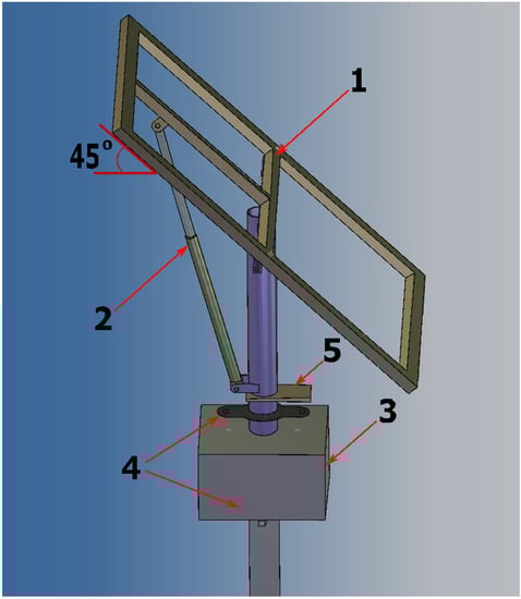
Figure 2.
The general structure of a single-axis solar tracker.
Figure 3 shows the internal rotation mechanism of the Sun tracking system. Here, (1) is the support tube holding the solar panel; (2) is the gear wheel (worm wheel) fixed to the support tube; (3) is the worm gear (worm and driveshaft) connected to the gear wheel (2); (4) is the DC motor SV35-130/HP5BFN controlling the rotation of the worm gear. This mechanism is more reliable in controlling the solar tracker, since the worm-rotating mechanism is more resistant to external dynamic forces (wind, manual rotation of the tracker). In this way, the tracker turns only when the DC motor turns on (rotates).

Figure 3.
Mechanism for rotating the tracker in a horizontal plane.
Figure 4 shows the structure of the encoder for determining the azimuth angle of the solar tracker rotation. Here, the main element is a stationary single-turn potentiometer (4) with resistance of 1 kOhm. The mechanical angle of rotation reaches , which is quite enough for our purposes. The installed gears (1) are the same size. One of the gears (3) is attached to the tracker’s support tube and rotates with the solar panel. All these components are located in the same block (2).
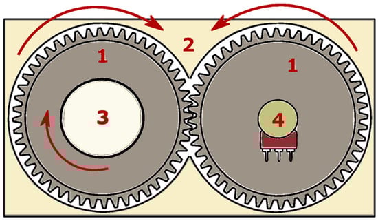
Figure 4.
The structure of the encoder.
The potentiometer is connected to the analog input of a microcontroller with a ten-bit ADC. Accordingly, the angle corresponds approximately to 0.185 mV.
3. Block Diagram of Electronic Control Units for Solar Trackers
This section will cover the control units of the studied solar tracking systems.
3.1. Solar Tracking System Based on Astronomical Calculations of the Sun’s Position
This method is based on astronomical calculations of the Sun’s trajectory relative to the Earth in the horizontal coordinate system (2) []:
where δ is the declination angle and d is the ordinal number of the current day of the year, so for 1 January, d = 1. The height of the Sun α is calculated as:
where φ is the latitude of the sun tracking system’s location and LST is the local solar time. Finally, the expression for the azimuth angle, :
Figure 5 shows the electronic unit of a single-axis solar tracking system for this method. The entire electronic circuit is powered by a 12 V battery (4). The circuit also has a 5 V (6) and 3.3 V (2) voltage stabilizer, which are respectively connected to the Atmega 328p (1) and an SD card (3) programmable microcontroller. The coordinates of the Sun’s movement are stored in the SD card. Using these data, as well as the DS1307 real-time clock (10), the microcontroller turns the motor at a certain angle through the l298n driver (11), directing the photovoltaic panel (13) towards the Sun. The rotation angle of the solar tracker is calculated through the encoder using a variable resistor (12). To measure the voltage on the solar battery, a voltage sensor is used, which is a voltage divider connected to the analog input of the microcontroller (8). To measure the current generated by the solar battery, a digital current sensor ACS712 (9) connected to the output of the solar panel is used. A 750 W rheostat (5) with a 30 Ohm rating was used as the load. All data from the installed sensors are sent to the dispatcher via a wireless channel using the LoRa E32-1W wireless module (7). Wireless modules with LoRa modulation (LongRange) have a high level of noise immunity and a relatively low level of energy consumption [].

Figure 5.
Functional diagram of the electronic control unit of a single-axis Solar tracking system based on astronomical calculations.
3.2. Solar Tracking System Based on Photosensitive Sensors
This method is based on the use of light-sensitive sensors, in our case, LDR. Figure 6 shows the control unit diagram of a single-axis solar tracking system based on photosensors. The tracker is controlled using the Atmega 328P (1) programmable microcontroller. The entire system is powered by a 12 V battery (5). Therefore, the microcontroller is powered via the LM7805 stabilizer (12). The upper part of the circuit (2) with the LM324 operational amplifier controls the rotation of the DC motor. Two photoresistors (3) are installed here to determine the intensity of solar radiation. The signals passing through the photoresistors are amplified by an operational amplifier to control the transistors. They, in turn, act as a key for the motor. A relay (4) is installed between the motor and the battery to avoid unnecessary energy consumption. The system also has an ACS712 digital current sensor (8) and a voltmeter (6). They measure the power of the electric current generated by the solar battery (9). The load for the solar panel is a rheostat (11) with a resistance of 30 Ohms and a power of 750 watts. To determine the exact orientation of the photovoltaic panel to the Sun, an encoder (7) was also installed here, but it does not affect the operation of this tracker. It is necessary to compare the rotation angles of the scheduled solar tracker and LDR solar tracker. All data from the sensors are sent to the microcontroller and are sent to the dispatcher using the LoRa E32-1W (10) wireless module.

Figure 6.
Functional diagram of the electronic control unit of a single-axis solar tracking system based on photoresistors.
4. Algorithms for Single-Axis Solar Tracking Systems
This section will cover the algorithms of the manufactured trackers.
4.1. Algorithm for a Single-Axis Solar Tracker Based on an Astronomical Date
Figure 7 shows a block diagram of the algorithm for a single-axis solar tracking system based on astronomical calculations. The system is autonomous. Using the built-in real-time sensor and SD card with the coordinates of the Sun’s movement, the system automatically sets the appropriate azimuth angles depending on the date and time.

Figure 7.
Algorithm for a single-axis solar tracker based on astronomical data.
After turning the system on, the microcontroller accesses the DS1307 real-time clock. Using the date (d) and time (t) as well as SD card data, the controller determines the azimuth and height of the Sun above the horizon. If the Sun has not yet risen, the system remains in the initial position. If the Sun has risen, the controller determines the azimuth angle γ of the Sun at a given time and starts turning the tracker to the desired angle. The tracker is rotated until the angle from the encoder is equal to the azimuthal angle of the Sun stored on the flash drive. Once installed in the desired position, the system measures the current (I) and voltage (U) of the solar panel. Next, data are sent to the dispatcher via a wireless channel using the LoRa wireless module. Then, the system goes into sleep mode for a certain adjustable period of time. The duty cycle is repeated until the microcontroller detects the sunset.
4.2. Algorithm for a Single-Axis Solar Tracker Based on Photosensors
Figure 8 shows a block diagram of the solar tracking system algorithm based on photoresistors. The microcontroller starts the system only when the light sensor detects the sunrise. Next, the controller switches on the relay for 1 min. At this time, the solar panel is oriented to the Sun. The tracker will only stop when the light intensities are equal. After 1 min, the microcontroller switches off the relay. When set to the desired position, the system measures the output current (I) and voltage (U) of the solar panel. The system also detects the azimuth angle of the solar tracker using an encoder. All sensor data are sent to the control center using the LoRa wireless modules. Then, the system goes into sleep mode for a certain adjustable period of time. The device has two tips (lock, button) to indicate the maximum azimuth angle of sunrise and sunset. These azimuth values were chosen for the summer and winter solstices on 22 June and 21 December. Azimuthal angles of sunrise and sunset for Almaty city on these days are and , respectively.

Figure 8.
Algorithm for a single-axis solar tracker based on photosensors.
5. Experimental Results and Discussion
Experimental work was carried out on the territory of the al-Farabi KazNU University, Almaty, in order to compare the generated power of the single-axis solar trackers with (based on schedule and LDR) time and photosensor management.
Figure 9 shows the experimental installations of single-axis solar trackers. SAKOPOLY-60W with output power 60 W was used as a solar panel. Solar panel specifications: maximum power current Imp—3.33 A; maximum power voltage Vmp—18.2 V; open circuit voltage Voc—22.7 V; short circuit current Isc—3.66 A. Here, (1) is a tracker that works with astronomical time; (2) is a tracker that works with a photosensitive sensor; (3) is a stationary photovoltaic installation; (4) is an electronic control unit; (5) is a load for a solar panel; (6) is a power source for an electronic unit.

Figure 9.
Experimental installations.
The experiment was conducted over five days, in various weather conditions. Measurements of voltage and current were conducted using embedded ADC of MCU and current sensor ACS712. Data from voltage and current sensors were delivered by LoRa wireless channel every 15 min during the whole experimental day. Figure 10a–e show graphs of solar panel power generation over 5 days in July 2020. Sharp dips in the charts due to strong light scattering correspond to the appearance of clouds in the sky. It can be seen from the graphs if the weather conditions are favorable, both trackers generate the same amount of energy. However, when weather conditions worsen and cloudiness, rain, or fog occur, differences appear in the generated energy graphs. The tracker based on astronomical calculations shows slightly better results. This is due to the fact that when the sun’s rays are scattered on clouds, photosensors are not able to accurately determine the position of the Sun; in this case, the solar panel may be directed in the opposite direction from the position of the Sun, which affects the generation of solar energy. Figure 11a–c show the rotation angles of the solar panels under strong scattering conditions obtained using encoders. These graphs show erroneous azimuth angles of solar tracker rotation with photosensors.
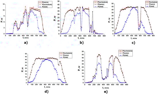
Figure 10.
Generation of energy on: (a) 1 July 2020, (b) 2 July 2020, (c) 3 July 2020, (d) 8 July 2020, (e) 9 July 2020.
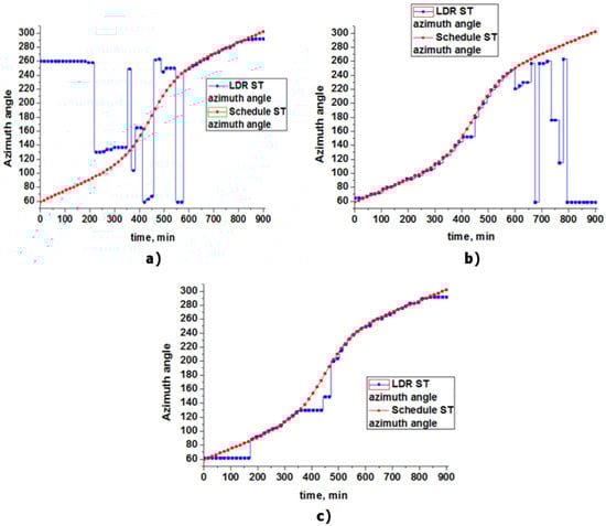
Figure 11.
The azimuthal angles of the trackers: (a) 1 July 2020, (b) 2 July 2020, (c) 9 July 2020.
6. The Calculation of the Efficiency
In order to determine the efficiency of the experimental installations, calculations were made for the total energy generation during the day, which is shown in Table 2. Here, Esc—energy of the schedule controlled solar tracker; ELDR—energy of solar tracker with LDR; Efix—energy of fixed solar panel.
Table 2.
Total amount of power generated by day.
The efficiency of the tracker can be estimated using the Equation (5): where ET is the energy generated by the solar tracker, EPV is the energy equivalent to a fixed photovoltaic panel without a tracker, and EC is the energy consumption for the tracker mechanism [,]:
To calculate the efficiency of solar trackers, it is also necessary to calculate the consumption of the tracker motors. Table 3 shows the values used to determine the consumption.
Table 3.
Power performance of motor.
The installation mechanism for turning the tracker by 1 degree consumes 0.823 joules. Table 4 shows the motor consumption of a schedule solar tracker. Here, is the total azimuthal angle of the Sun from sunrise to sunset; E—the energy required to rotate the tracker to the total azimuthal angle; tr—time to turn the tracker on a total azimuth angle; Pr is the power consumed by the mechanism of the tracker. The resulting energy values should be doubled since the tracker returns to its original position at the end of each day.
Table 4.
Power consumption of schedule solar tracker’s motor.
The amount of energy consumed for 5 days of the experiment was 0.557 Wh, and the efficiency of the tracker based on astronomical calculations was 57.4%, taking into account the energy consumption for the rotation mechanism.
Next, two trackers are compared using expression (5). The efficiency of schedule ST compared to LDR ST was 4.2% on cloudy and rainy days, and on days with variable cloud cover, it is 1.15%. The consumption of the schedule ST motor is 60% less than that of the LDR ST motor due to errors in determining the position of the Sun by photosensors.
7. Modeling the Performance of the Tracker Taking into Account the Weather Conditions during the Year
The climate in Almaty city is sharply continental—all four seasons are pronounced here, with frequent clouds and rapid weather condition changes. As a result, the design of solar power plants using single-axis trackers requires an assessment of their performance. To simulate the performance of a schedule ST and LDR ST, it is necessary to estimate the change in radiation levels under different weather conditions. In order to determine the solar radiation coming to the Earth’s surface during the day, experiments were performed using an autonomous wireless installation with a pyranometer for 5 days in August 2020. The obtained data were used to estimate the reduction in the radiation power level in cloudy and rainy weather. To determine how much the performance of photovoltaic systems decreases in various weather conditions, the model of solar radiation per square meter of the horizontal surface during the year was used. The total radiation (G) coming from the Sun can be calculated using the formula (6) []:
where n is the ordinal number of the day in the year, T is the local time, and k is the correction factor depending on climatic conditions []; —correction factor for the distance from the Earth to the Sun; I0—constant solar radiation 1.37 kW/m2; —the influence of the angle of the panel; —the influence of the azimuthal angle; hs—the height of Sun.
Figure 12 shows graphs of solar radiation received from the pyranometer as well as models of radiation on the same days. The graph of the mathematical model of solar radiation from 18 to 24 August has no changes, while the graphs obtained using the pyranometer strongly depend on weather conditions. Using experimental data and a mathematical model, the average degree of decrease in solar radiation power Δχ is calculated to predict incoming radiation under adverse weather conditions. If it is represented as an array with i rows equal to the number of days under consideration and j columns equal to the number of radiation measurements during the day, the matrix (7) is obtained:
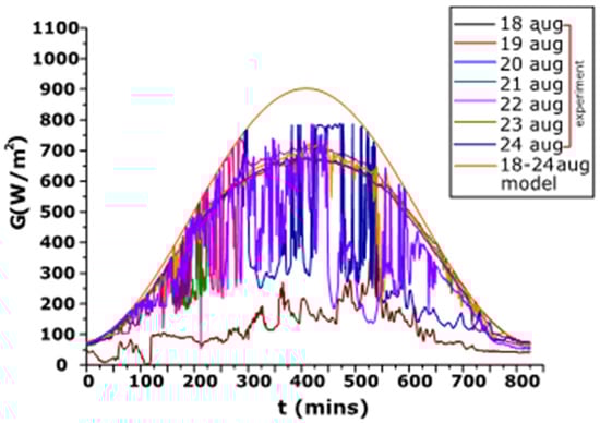
Figure 12.
Radiation values of the experiment (the first specified dates from 18 to 24 August) and the model (the lower specified dates from 18 to 24 August).
In the same way, a matrix is constructed for the power values obtained from formula (6).
Therefore, the time intervals for the matrixes (7) and (8) are the same. Next, a set of matrix elements (7) in each row is selected, having a low level of solar radiation due to clouds gexp and obtaining an array with the number of elements n. The same elements are selected from the matrix (8) for the gmodel array. Then, the average share of solar radiation in adverse conditions Δχ during the day can be expressed as:
Here, is the average coefficient for adverse weather conditions.
As a result of the calculations, the following coefficient values were obtained:
- In rainy weather conditions, the solar radiation level is 0.2 of the calculated Gmodel value on a corresponding day;
- In cloudy weather, the solar radiation level is 0.45 of the calculated Gmodel value on a corresponding day;
- On days with variable cloud cover, the solar radiation flux reaches 0.66 of the calculated Gmodel on a corresponding day.
Using the obtained coefficients for various weather conditions, the radiation level was calculated for the 2019 year. Weather conditions for the year were obtained from an internet resource []. Figure 13 shows radiation graphs for the 2019 year under ideal conditions and taking into account coefficients for various weather conditions.

Figure 13.
Calculated annual solar radiation under ideal conditions and taking into account weather conditions.
Using data from annual solar radiation, the amount of electrical energy generated by solar trackers is calculated.
Figure 14 shows dependence graphs of energy generated by trackers during 2019, taking into account coefficients for various weather conditions.

Figure 14.
Calculated annual solar radiation under ideal conditions and weather conditions.
Table 5 shows the estimated amount of energy generated by solar trackers in various weather conditions.
Table 5.
Estimated amount of energy generated by solar trackers in various weather conditions.
As can be seen from Table 5, the number of clear days is slightly higher than the number of cloudy and rainy days. Consequently, the amount of energy produced by trackers on these days will differ.
The results obtained in this work can be used in the design of solar trackers in areas with variable climatic conditions.
8. Conclusions
As a result of this work, it was found that the schedule-based solar tracking system is 4.2% more efficient than LDR solar trackers in different weather conditions. The proposed tracker showed 57.4% more efficiency compared with a fixed solar panel set to optimal tilt angle. Wrong determination of the Sun’s position by the LDR tracker in cloudy or rainy weather leads to a decrease in the power of the solar panel. In addition, as a result of this work, a mechanism was developed using an encoder for accurate determination of the azimuth angle of the Sun. This mechanism is a trade-off between accuracy and simplicity and the cost of necessary equipment. Based on the experimental data, the output power of solar trackers was calculated during the year. The obtained results can be used in the design of solar trackers in areas with a variable climate.
Author Contributions
Conceptualization, N.K., A.S. and S.M.; methodology, N.K. and M.N.; software, D.T.; validation, G.D. and Y.S.; investigation, N.K and M.N.; data curation, Y.S. and G.D.; writing—original draft preparation, N.K.; visualization, A.M.; supervision, A.S. and S.M.; project administration, A.S. All authors have read and agreed to the published version of the manuscript.
Funding
This work has been supported financially by the research project AP05132464 of the Ministry of Education and Science of the Republic of Kazakhstan and was performed at Research Institute of Mathematics and Mechanics in al-Farabi Kazakh National University, which is gratefully acknowledged by the authors.
Acknowledgments
We acknowledge the administration of Research Institute of Mathematics and Mechanics in al-Farabi Kazakh National University for support and assistance.
Conflicts of Interest
The authors declare no conflict of interest.
References
- Mwasilu, F.; Justo, J.J.; Kim, E.-K.; Do, T.D.; Jung, J.-W. Electric vehicles and smart grid interaction: A review on vehicle to grid and renewable energy sources integration. Renew. Sustain. Energy Rev. 2014, 34, 501–516. [Google Scholar] [CrossRef]
- Rodrigues, S.; Torabikalaki, R.; Faria, F.; Cafôfo, N.; Chen, X.; Ivaki, A.R.; Mata-Lima, H.; Morgado-Dias, F. Economic feasibility analysis of small scale PV systems in different countries. Sol. Energy 2016, 131, 81–95. [Google Scholar] [CrossRef]
- Saymbetov, A.K.; Nurgaliyev, M.K.; Nalibayev, Y.D.; Kuttybay, N.B.; Svanbayev, Y.A.; Dosymbetova, G.B.; Tulkibaiuly, Y.; Meiirkhanov, A.K.; Kopzhan, Z.K.; Gaziz, K.A. Intelligent Energy Efficient Wireless Communacation System for Street Lighting. In Proceedings of the International Conference on Computing and Network Communications (CoCoNet), Astana, Kazakhstan, 15–17 August 2018. [Google Scholar]
- Tukymbekov, D.; Saymbetov, A.; Nurgaliyev, M.; Kuttybay, N.; Nalibayev, Y.; Dosymbetova, G. Intelligent energy efficient street lighting system with predictive energy consumption. In Proceedings of the International Conference on Smart Energy Systems and Technologies (SEST), Porto, Portugal, 9–11 September 2019. [Google Scholar]
- Singh, R.; Kumar, S.; Gehlot, A.; Pachauri, R. An imperative role of sun trackers in photovoltaic technology: A review. Renew. Sustain. Energy Rev. 2018, 82, 3263–3278. [Google Scholar] [CrossRef]
- Kuttybay, N.; Mekhilef, S.; Saymbetov, A.; Nurgaliyev, M.; Meiirkhanov, A.; Dosymbetova, G.; Kopzhan, Z. An Automated Intelligent Solar Tracking Control System with Adaptive Algorithm for Different Weather Conditions. In Proceedings of the 2019 IEEE International Conference on Automatic Control and Intelligent Systems (I2CACIS), Shah Alam, Selangor, 29 June 2019. [Google Scholar]
- Mousazadeh, H.; Keyhani, A.; Javadi, A.; Mobli, H.; Abrinia, K.; Sharifi, A. A review of principle and sun-tracking methods for maximizing solar systems output. Renew. Sustain. Energy Rev. 2009, 13, 1800–1818. [Google Scholar] [CrossRef]
- Saymbetov, A.K.; Nurgaliyev, M.K.; Tulkibaiuly, Y.; Toshmurodov, Y.K.; Nalibayev, Y.D.; Dosymbetova, G.B.; Kuttybay, N.B.; Gylymzhanova, M.M.; Svanbayev, Y.A. Method for Increasing the Efficiency of a Biaxial Solar Tracker with Exact Solar Orientation. Appl. Sol. Energy 2018, 54, 126–130. [Google Scholar] [CrossRef]
- Senpinar, A.; Cebeci, M. Evaluation of power output for fixed and two-axis tracking PVarrays. Appl. Energy 2012, 92, 677–685. [Google Scholar] [CrossRef]
- Huang, B.; Sun, F. Feasibility study of one axis three positions tracking solar PV with low concentration ratio reflector. Energy Convers. Manag. 2007, 48, 1273–1280. [Google Scholar] [CrossRef]
- Nsengiyumva, W.; Chen, S.G.; Hu, L.; Chen, X. Recent advancements and challenges in Solar Tracking Systems (STS): A review. Renew. Sustain. Energy Rev. 2018, 81, 250–279. [Google Scholar] [CrossRef]
- Gil, F.G.; Martin, M.D.S.; Vara, J.P.; Calvo, J.R.; Perlovsky, L.; Dionysiou, D.D.; Mastorakis, N.E. A review of solar tracker patents in Spain. In Proceedings of the 3rd WSEAS International Conference on Energy Planning, Energy Saving, Environmental Education, EPESE ’09, 3rd WSEAS International Conference on Renewable Energy Sources, RES ’09, 3rd WSEAS International Conference on Waste Management, WWAI ’09, Canary Islands, Spain, 1–3 July 2009; pp. 292–297. [Google Scholar]
- Helwa, N.H.; Bahgat, A.B.G.; El Shafee, A.M.R.; El Shenawy, E.T. Computation of the Solar Energy Captured by Different Solar Tracking Systems. Energy Sources 2000, 22, 35–44. [Google Scholar] [CrossRef]
- Helwa, N.H.; Bahgat, A.B.G.; El Shafee, A.M.R.; El Shenawy, E.T. Maximum Collectable Solar Energy by Different Solar Tracking Systems. Energy Sources 2000, 22, 23–34. [Google Scholar] [CrossRef]
- Gordon, J.; Wenger, H.J. Central-station solar photovoltaic systems: Field layout, tracker, and array geometry sensitivity studies. Sol. Energy 1991, 46, 211–217. [Google Scholar] [CrossRef]
- Gay, C.F.; Yerkes, J.W.; Wilson, J.H. Performance advantages of two-axis tracking for large flat-plate photovoltaic energy systems. In Proceedings of the Photovoltaic Specialists Conference, Record (A84-22957 09-44), San Diego, CA, USA, 27–30 September 1982; Volume 16, pp. 1368–1371. [Google Scholar]
- Koussa, M.; Cheknane, A.; Hadji, S.; Haddadi, M.; Noureddine, S. Measured and modelled improvement in solar energy yield from flat plate photovoltaic systems utilizing different tracking systems and under a range of environmental conditions. Appl. Energy 2011, 88, 1756–1771. [Google Scholar] [CrossRef]
- Alexandru, C.; Tatu, N.I. Optimal design of the solar tracker used for a photovoltaic string. J. Renew. Sustain. Energy 2013, 5, 23133. [Google Scholar] [CrossRef]
- Li, Z.; Liu, X.; Tang, R. Optical performance of inclined south-north single-axis tracked solar panels. Energy 2010, 35, 2511–2516. [Google Scholar] [CrossRef]
- Li, Z.; Liu, X.; Tang, R. Optical performance of vertical single-axis tracked solar panels. Renew. Energy 2011, 36, 64–68. [Google Scholar] [CrossRef]
- Fahad, H.M.; Islam, A.; Islam, M.; Hasan, F.; Brishty, W.F.; Rahman, M. Comparative Analysis of Dual and Single Axis Solar Tracking System Considering Cloud Cover. In Proceedings of the International Conference on Energy and Power Engineering (ICEPE), Dhaka, Bangladesh, 14–16 March 2019. [Google Scholar]
- Al-Rousan, N.; Isa, N.A.M.; Desa, M.K.M. Advances in solar photovoltaic tracking systems: A review. Renew. Sustain. Energy Rev. 2018, 82, 2548–2569. [Google Scholar] [CrossRef]
- Huang, B.; Ding, W.; Huang, Y. Long-term field test of solar PV power generation using one-axis 3-position sun tracker. Sol. Energy 2011, 85, 1935–1944. [Google Scholar] [CrossRef]
- Kacira, M.; Simsek, M.; Babur, Y.; Demirkol, S. Determining optimum tilt angles and orientations of photovoltaic panels in Sanliurfa, Turkey. Renew. Energy 2004, 29, 1265–1275. [Google Scholar] [CrossRef]
- Huang, B.-J.; Huang, Y.-C.; Chen, G.-Y.; Hsu, P.-C.; Li, K. Improving Solar PV System Efficiency Using One-Axis 3-Position Sun Tracking. Energy Procedia 2013, 33, 280–287. [Google Scholar] [CrossRef]
- Chang, T.P. Performance study on the east–west oriented single-axis tracked panel. Energy 2009, 34, 1530–1538. [Google Scholar] [CrossRef]
- Al-Mohamad, A. Efficiency improvements of photo-voltaic panels using a Sun-tracking system. Appl. Energy 2004, 79, 345–354. [Google Scholar] [CrossRef]
- Lorenzo, E.; Pérez, M.; Ezpeleta, A.; Acedo, J. Design of tracking photovoltaic systems with a single vertical axis. Prog. Photovolt. Res. Appl. 2002, 10, 533–543. [Google Scholar] [CrossRef]
- Obara, S.; Matsumura, K.; Aizawa, S.; Kobayashi, H.; Hamada, Y.; Suda, T. Development of a solar tracking system of a nonelectric power source by using a metal hydride actuator. Sol. Energy 2017, 158, 1016–1025. [Google Scholar] [CrossRef]
- Lazaroiu, G.C.; Longo, M.; Roscia, M.; Pagano, M. Comparative analysis of fixed and sun tracking low power PV systems considering energy consumption. Energy Convers. Manag. 2015, 92, 143–148. [Google Scholar] [CrossRef]
- Sefa, I.; Demirtaş, M.; Çolak, I. Application of one-axis sun tracking system. Energy Convers. Manag. 2009, 50, 2709–2718. [Google Scholar] [CrossRef]
- Chin, C.S.; Babu, A.; McBride, W. Design, modeling and testing of a standalone single axis active solar tracker using MATLAB/Simulink. Renew. Energy 2011, 36, 3075–3090. [Google Scholar] [CrossRef]
- Hoffmann, F.M.; Molz, R.F.; Kothe, J.V.; Nara, E.O.B.; Tedesco, L.P.C. Monthly profile analysis based on a two-axis solar tracker proposal for photovoltaic panels. Renew. Energy 2018, 115, 750–759. [Google Scholar] [CrossRef]
- Yilmaz, S.; Ozcalik, H.R.; Dogmus, O.; Dincer, F.; Akgol, O.; Karaaslan, M. Design of two axes sun tracking controller with analytically solar radiation calculations. Renew. Sustain. Energy Rev. 2015, 43, 997–1005. [Google Scholar] [CrossRef]
- Barsoum, N. Fabrication of Dual-Axis Solar Tracking Controller Project. Intell. Control. Autom. 2011, 2, 57–68. [Google Scholar] [CrossRef]
- El Kadmiri, Z.; El Kadmiri, O.; Masmoudi, L.; Bargach, M.N. A Novel Solar Tracker Based on Omnidirectional Computer Vision. J. Sol. Energy 2015, 2015, 1–6. [Google Scholar] [CrossRef]
- Tudorache, T.; Kreindler, L. Design of a solar tracker system for PV power plants. Acta Polytech. Hung. 2010, 7, 23–39. [Google Scholar]
- Pattanasethanon, S. The Solar Tracking System by Using Digital Solar Position Sensor. Am. J. Eng. Appl. Sci. 2010, 3, 678–682. [Google Scholar] [CrossRef]
- Algarin, R.; Arturo, C.; Castro, A.J.O.; Casas, J.N. Dual-axis solar tracker for using in photovoltaic systems. Int. J. Renew. Energy 2017, 7, 137–145. [Google Scholar]
- Sungur, C. Multi-axes sun-tracking system with PLC control for photovoltaic panels in Turkey. Renew. Energy 2009, 34, 1119–1125. [Google Scholar] [CrossRef]
- Roth, P.; Georgiev, A.; Boudinov, H. Cheap two axis sun following device. Energy Convers. Manag. 2005, 46, 1179–1192. [Google Scholar] [CrossRef]
- Kamala, J.; Joseph, A. Solar tracking for maximum and economic energy harvesting. Int. J. Eng. Technol. 2014, 5, 5030–5037. [Google Scholar]
- Ranganathan, R.; Mikhael, W.; Kutkut, N.; Batarseh, I. Adaptive sun tracking algorithm for incident energy maximization and efficiency improvement of PV panels. Renew. Energy 2011, 36, 2623–2626. [Google Scholar] [CrossRef]
- Nayak, S.R. Solar Tracking Application. IOSR J. Eng. 2012, 2, 1278–1281. [Google Scholar] [CrossRef]
- Sidek, M.; Azis, N.; Hasan, W.; Ab Kadir, M.; Shafie, S.; Radzi, M. Automated positioning dual-axis solar tracking system with precision elevation and azimuth angle control. Energy 2017, 124, 160–170. [Google Scholar] [CrossRef]
- Gregor, R.; Takase, Y.; Rodas, J.; Carreras, L.; Gregor, D.; López, A. Biaxial Solar Tracking System Based on the MPPT Approach Integrating ICTs for Photovoltaic Applications. Int. J. Photoenergy 2015, 2015, 1–10. [Google Scholar] [CrossRef]
- Fathabadi, H. Novel high efficient offline sensorless dual-axis solar tracker for using in photovoltaic systems and solar concentrators. Renew. Energy 2016, 95, 485–494. [Google Scholar] [CrossRef]
- Tharamuttam, J.K.; Ng, A.K. Design and Development of an Automatic Solar Tracker. Energy Procedia 2017, 143, 629–634. [Google Scholar] [CrossRef]
- Ho, M.-C.; Lai, A.-C.; Chong, K.-K.; Tan, M.-H.; Lim, B.H.; King, Y.J.; Lee, J.-V. Design and Construction of Prototype Mobile Sun-Tracking System for Concentrator Photovoltaic System. Energy Procedia 2017, 142, 736–742. [Google Scholar] [CrossRef]
- Jiang, X.; Zhang, J.; Harding, B.J.; Makela, J.J.; Domínguez-García, A.D. Spoofing GPS Receiver Clock Offset of Phasor Measurement Units. IEEE Trans. Power Syst. 2013, 28, 3253–3262. [Google Scholar] [CrossRef]
- Zhang, Z.; Gong, S.; Dimitrovski, A.; Li, H. Time Synchronization Attack in Smart Grid: Impact and Analysis. IEEE Trans. Smart Grid 2013, 4, 87–98. [Google Scholar] [CrossRef]
- Skvortzov, V.Y.; Lee, H.-K.; Bang, S.; Lee, Y. Application of Electronic Compass for Mobile Robot in an Indoor Environment. In Proceedings of the 2001 IEEE International Conference on Robotics and Automation, Seoul, Korea, 21–26 May 2001. [Google Scholar]
- Cho, S.Y.; Park, C.G. Tilt compensation algorithm for 2-axis magnetic compass. Electron. Lett. 2003, 39, 1589. [Google Scholar] [CrossRef]
- Ojeda, L.; Borenstein, J. Experimental results with the KVH C-100 fluxgate compass in mobile robots. In Proceedings of the IASTED International Conference on Robotics and Applications, Honolulu, HI, USA, 14–16 August 2000. [Google Scholar]
- Kwon, W.; Roh, K.-S.; Sung, H.-K. Particle filter-based heading estimation using magnetic compasses for mobile robot navigation. In Proceedings of the IEEE International Conference on Robotics and Automation, Orlando, FL, USA, 15–18 May 2006. [Google Scholar]
- Lee, K.; Kim, Y.; Yun, J.; Lee, J. Magnetic-interference-free dual-electric compass. Sens. Actuators A Phys. 2005, 120, 441–450. [Google Scholar] [CrossRef]
- Nurgaliyev, M.; Saymbetov, A.; Yashchyshyn, Y.; Kuttybay, N.; Tukymbekov, D. Prediction of energy consumption for LoRa based wireless sensors network. Wirel. Netw. 2020, 26, 3507–3520. [Google Scholar] [CrossRef]
- Ioniţă, M.A.; Alexandru, C. Dynamic optimization of the tracking system for a pseudo-azimuthal photovoltaic platform. J. Renew. Sustain. Energy 2012, 4, 053117. [Google Scholar] [CrossRef]
- Zhang, P.; Zhou, G.; Zhu, Z.; Li, W.; Cai, Z. Numerical study on the properties of an active sun tracker for solar streetlight. Mechatronics 2013, 23, 1215–1222. [Google Scholar] [CrossRef]
- Zhu, Y.; Liu, J.; Yang, X. Design and performance analysis of a solar tracking system with a novel single-axis tracking structure to maximize energy collection. Appl. Energy 2020, 264, 114647. [Google Scholar] [CrossRef]
- World-weather.ru. Available online: https://world-weather.ru/pogoda/kazakhstan/almaty/ (accessed on 6 September 2020).
© 2020 by the authors. Licensee MDPI, Basel, Switzerland. This article is an open access article distributed under the terms and conditions of the Creative Commons Attribution (CC BY) license (http://creativecommons.org/licenses/by/4.0/).