Abstract
In 2019, the Event Horizon Telescope (EHT) released the first image of a black hole, sparking huge interest in the study of black-hole images. We present analytical solutions to the null geodesic equations for Kerr–Newman–de Sitter black holes derived using Jacobi elliptic functions. Using these solutions, we have performed an analytic ray-tracing simulation to model direct images, lensing rings, and photon rings, considering standard observers and zero angular momentum observers (ZAMOs). Additionally, we have derived analytic expressions for the critical parameters governing the structure of the photon ring and analyzed them in detail. From the foregoing, an increase in charge leads to a decrease in both time delay and Lyapunov exponent, while the change in azimuthal angle is insignificant. These findings improve our understanding of the effects of charge on black-hole photon rings and provide a foundation for future studies.
1. Introduction
General relativity (GR) stands as the preeminent theory of gravity, extensively corroborated through its capacity to elucidate an array of astrophysical phenomena. According to the uniqueness theorems, black holes are characterized exclusively by mass, angular momentum, and electromagnetic charge, often encapsulated by the “no-hair” theorem. Nevertheless, whether black holes are described by the Kerr solution or alternative solutions within or beyond the gr framework remains an open question.
Evidence from observations coming from a variety of cosmological probes has perpetually highlighted the existence of dark energy, a cryptic entity responsible for the universe’s accelerating expansion. The cosmological constant provides a simple and elegant explanation for observed acceleration, thereby presenting an appealing option for further investigation. Furthermore, it is feasible to presume that black holes are slightly charged, making it worthwhile to investigate how this affects their observational characteristics. The Kerr–Newmann–de Sitter solution is a black-hole model that takes into consideration both charge and the cosmological constant. This research project seeks to examine the effect of charge and the cosmological constant on a black-hole photon ring.
The Event Horizon Telescope (EHT) collaboration has recently conducted groundbreaking interferometric observations of the supermassive black holes M87* and Sagittarius (Sgr) at the centers of Messier 87 and the Milky Way, respectively [1,2]. These observations have provided unprecedented insights into the emission structure on horizon scales. The relentless pursuit of enhanced image resolution and unprecedented levels of detail persists, propelled by the ongoing endeavors of the next-generation EHT [3]. Through these endeavors, the next-generation EHT aims to achieve the remarkable feat of capturing dynamic and high-resolution cinematic representations of black holes. This raises the questions:
- What can be anticipated as the resolution improves?
- What knowledge can be gleaned from such increasingly precise observations?
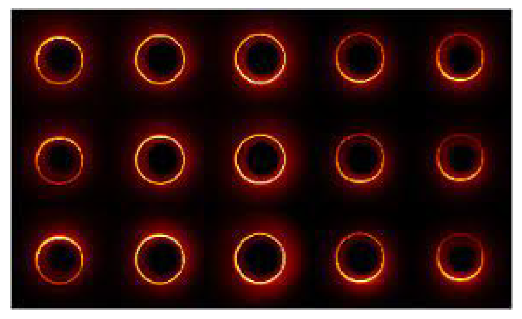
Simulations employing general relativistic magnetohydrodynamics (grMHD) demonstrate that the appearance of a black hole, if high resolution were achieved, would be dominated by a conspicuous presence of a thin and bright ring, aptly christened the “photon ring”, as illustrated in Figure 1.
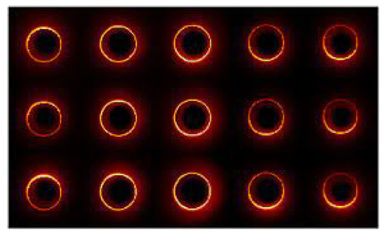
Figure 1.
General relativistic magnetohydrodynamic simulations of black-hole images [4].
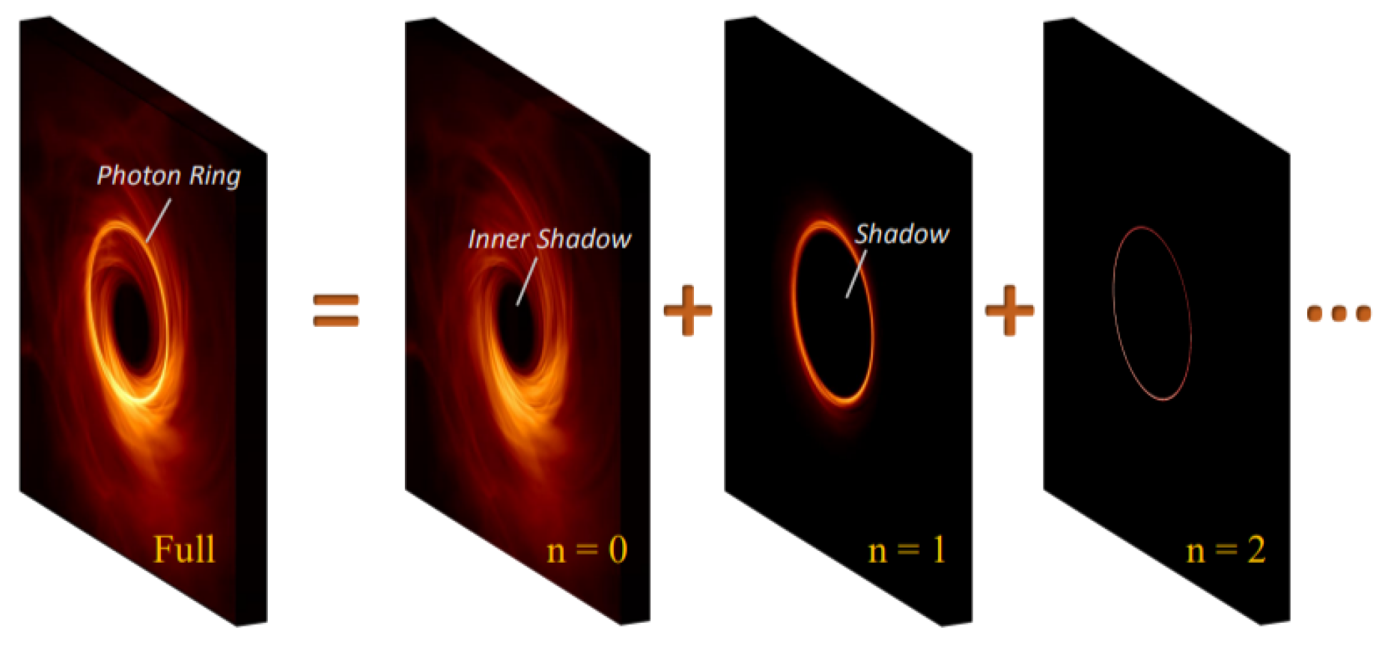
The existence of the photon ring is a categorical outcome of the strong gravity of the black hole, rendering it impervious to the details of the astrophysical source profile around the black hole. Calculations within the framework of gr unmask a captivating revelation: the photon ring, rather than being a single continual entity, unveils itself as a nested sequence of self-similar subrings, as illustrated in Figure 2.
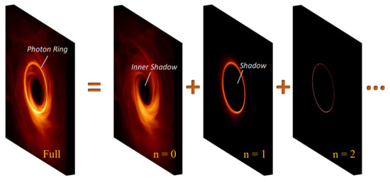
Figure 2.
Series of subrings in the black-hole image [3].
The subsequent subrings are exponentially demagnified and progressively converge to the critical curve. The very essence of the critical curve’s geometry is a candid manifestation of the black hole’s mass, spin, and the observer’s inclination, all intricately interwoven within the framework of gr. If the black hole’s metric encompasses additional parameters, the critical curve may undergo deviations from its gr archetype. Despite the undeniable significance of the critical curve, it is in itself not directly observable. Notably, unlike the critical curve, the photon ring bestows upon us a remarkable advantage—it is directly observable. Therefore, delving into the investigation of the photon ring unveils a captivating arena to peer deeply into gravity’s nature in the vicinity of black holes, both theoretically and experimentally.
Observational evidence from a wide range of cosmological probes [5,6] has consistently pointed to the existence of dark energy, an elusive entity responsible for the universe’s accelerating expansion. Because it provides a simple and elegant solution to the observed acceleration, the cosmological constant is a natural candidate for deciphering this phenomenon. Besides, it is important to highlight the physical interpretation of the cosmological constant considered in this work. In 1934, Lemaître proposed that the cosmological constant represents the energy density of a Lorentz Invariant Vacuum Energy (LIVE). He further argued that if the velocity relative to the vacuum energy is not measurable, its mass per unit volume will remain constant during the adiabatic expansion of a spatially homogeneous universe. Moreover, it is plausible to presuppose that black holes are somewhat charged, making it noteworthy to study how this affects their observational features. The Kerr–Newmann–de Sitter solution is a black-hole solution that takes into account both charge and cosmological constant. Apart from charge and Lorentz Invariant Vacuum Energy (LIVE), Kerr–Newman–de Sitter (KNdS) also accommodates the spin of the black hole. The presence of these three parameters complicates the geodesics, motivating us to derive its analytical solutions to gain a deeper understanding of this solution (KNdS). Additionally, in comparison to numerical analysis, which requires extensive computational power and is prone to errors, these analytical solutions help in explicitly understanding these geodesics by giving us more insights into the physics around the black hole.
Articles that have attempted ray-tracing in (KNdS) black holes include [7], where the authors conducted ray-tracing numerically, which is computationally expensive and lacks the precision required to resolve the individual photon rings corresponding to different orbital counts of the photons. For example, in the case of spin zero, the authors attempt an analytical approach using Weierstrass’ elliptic functions, which they note is more efficient for shadow modeling, since it avoids the need to compute full photon paths. By deriving exact analytic solutions using Jacobi elliptic functions, we achieve higher precision in ray-tracing without relying on computationally expensive methods. Additionally, our analytical framework allows for the separation of photon rings based on the number of photon orbits around the black hole, which was not resolved in [7]. Furthermore, the use of analytical solutions allows us to go a step further by investigating the underlying parameters that control the structure of the photon ring, such as the time delay, Lyapunov exponent, and change in azimuthal angle, which cannot be extracted through numerical methods. The analytical framework provides explicit functional forms of these parameters, revealing their dependence on black-hole spin, charge, and the cosmological constant. As a result, this work provides an avenue for investigating the photon rings and critical parameters in KNdS, which are important in the tests of general relativity as they present the physical observables that can be detected by the next-generation event horizon telescope [8].
The goal of this paper is to investigate the effect of charge and the cosmological constant on the black-hole photon ring. This work is organized as follows: In Section 2, we begin with a brief overview of the Kerr–Newmann–de Sitter solution. In Section 3, we proceed to investigate direct images, lensing rings, and the photon rings. Furthermore, we explore the critical parameters governing the structure of the images in Section 4 and give a conclusion of our results in Section 5. In the Section 5, we present the relevant calculation framework that has been used to obtain the solutions of various sections.
2. Overview of the Kerr–Newmann–De Sitter Solution
KNdS is one of the most general stationary, axially symmetric type D solutions of the Einstein–Maxwell equations in general relativity that describes the spacetime geometry in the region surrounding an electrically charged, rotating black hole. It generalizes the Kerr–Newman metric by taking into account the cosmological constant . In Boyer Lindquist coordinates, the metric is given by the line element [9],
where
Rescaled units are used so that the speed of light and gravitational constants are normalized (c = 1, G = 1). The metric depends on four parameters, namely the mass m, the spin a, a parameter for electric and magnetic charge and the cosmological constant . For , (1) reduces to the Reissner–Nordström–de Sitter metric [10] while in the uncharged case, we have the Kerr–de Sitter (KdS) (, ) or Schwarzschild–de Sitter (, a = 0) solutions [11].
Four fundamental quantities determine the equations of motion of photons: the Lagrangian, Carter’s constant Q, energy E, and the angular momentum in the z axis . and E are due to the axial symmetry and stationarity of the black-hole solution, while Q is associated with the hidden symmetry in KNdS spacetime. In the case of photons, only the sign of E has a physical meaning, hence the quantities , Q and E can be reparametrized as,
Null geodesics in KNdS spacetime in terms of these parameters are then given by,
where represents the four momenta along the photon’s trajectory.
To decouple (3)–(5), the Mino time parameter is introduced and defined as:
With which the decoupled equations become,
where
With the subscripts o and s denoting the observer and the source, respectively, and the Mino parameter is related to the integrals through the relationship;
Solutions to these integrals have been expressed in terms of Jacobi elliptic functions in Appendix B.
2.1. Analysis of the Angular Potential
In this subsection, we will do a brief analysis of the angular potential to acquire a grasp of various properties that will be useful in the subsequent sections. The angular potential has been given in Equation (11). Making use of the substitution on Equation (11) results in,
Solving for the roots gives,
where
Thus, the roots in terms of will be given by inverting which results in,
Equation (17) represents the turning points that a photon encounters in the latitudinal direction. The nature of the roots of Equation (17) can be investigated using the relation,
If , then whereby and . Mathematically, this implies that and will be real, while and will be complex. Physically, the photon will oscillate between and , which is the ordinary type of motion. In the ordinary type of motion, the photon crosses the equatorial plane each time as . Furthermore, if , then which implies that and . This means that all the roots will be real. In this case, the photon will either oscillate between and or and . This type of motion is referred to as vortical motion. In vortical motion, the photon is confined on one hemisphere since and or and . In the case that , then which gives rise to motion confined on the equatorial plane.
2.2. Analysis of the Radial Potential
In this subsection, we will conduct an analysis of the radial potential to gain insights into the important features that arise as a result of this potential. Focus will be given to the aspects that are relevant to the subsequent sections. The radial potential is as expressed in Equation (10), and its roots have been calculated in Appendix A. The roots represent the turning points that a photon encounters in the exterior of a black hole before escaping towards an observer, or, if there is no turning point in the exterior, the photon will plunge into the black hole. In the special case that a photon is bound at a constant radius in the exterior of a black hole, we have that . This is the mathematical condition for the existence of bound photon orbits. Using this condition, the constants of motion for bound photon orbits can be analytically obtained as follows:
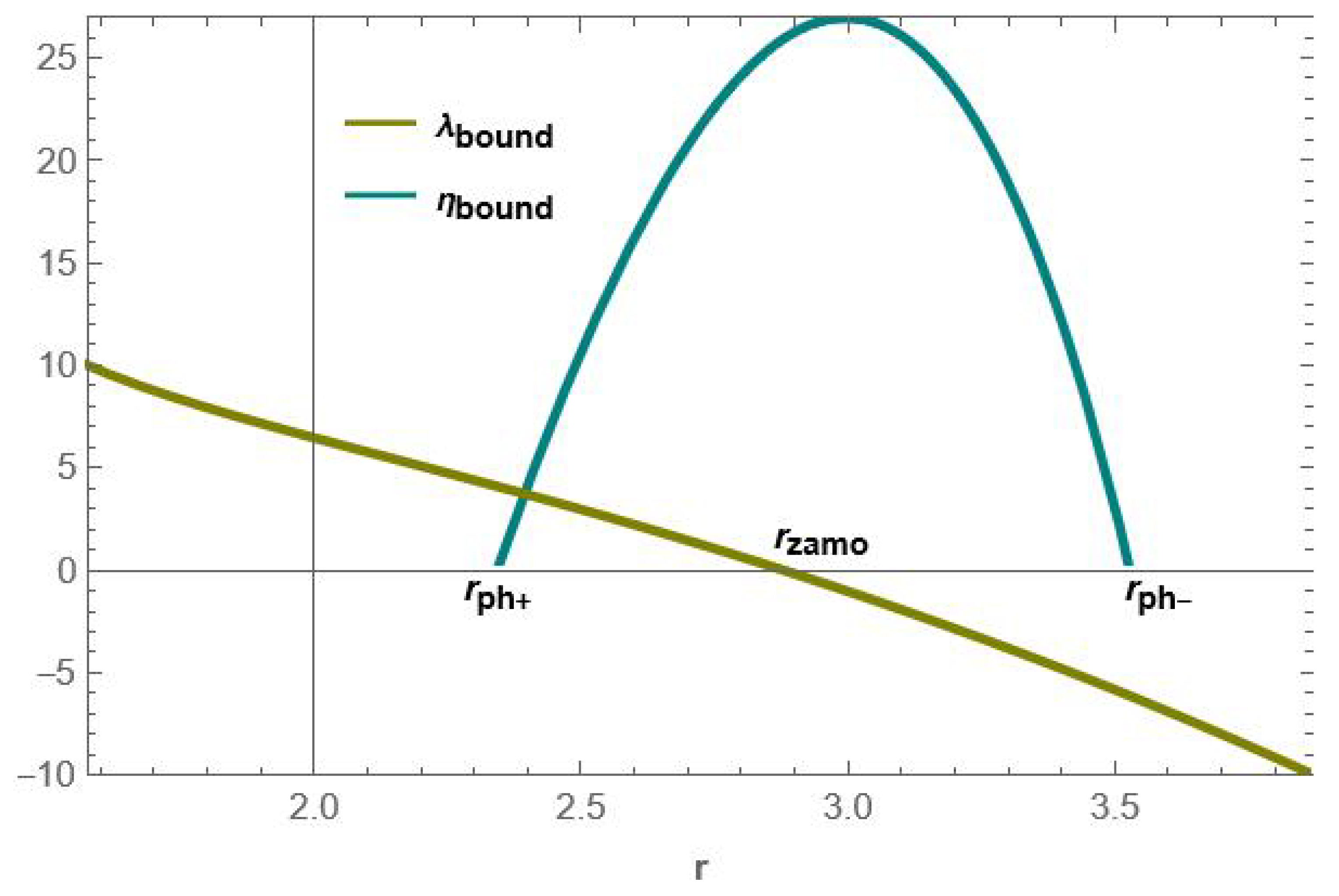
Using these constants of motion, Equations (19) and (20), various important aspects of bound photon orbits can be obtained. An illustration of these parameters is as shown in Figure 3.
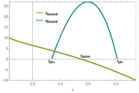
Figure 3.
Illustration of the constants of motion. In this plot, we have set , and .
The general behavior of is that it monotonically increases from zero to a maximum, where it again begins to monotonically decrease to zero. The points where form the lower and upper bounds in the exterior of a black hole where bound photon orbits can exist. These two radii, where , are referred to as the radius of equatorial bound photon orbits. We, respectively, denote them as and . The region is known as the photon region.
The parameter , on the other hand, monotonically decreases from positive values to negative values. The radial point where this parameter vanishes is known as the radius of the zero angular momentum orbit (). This radial point marks the region of transition of the orbits from co-rotating to counter-rotating orbits. Therefore, in the region of co-rotating orbits, , photons move with positive angular momentum in the azimuthal direction. On the other hand, in the region of counter-rotating orbits, , photons move with negative angular momentum in the z direction. By co-rotating, we mean that the photons move on orbits that are in the same direction as the direction of rotation of the black hole. By counter-rotating, we mean that photons move on orbits that are aligned in the opposite direction to the rotation of the black hole.
3. Direct Images, Lensing Rings, and Photon Rings
Our approach of constructing the direct images, lensing rings, and photon rings will consider locally static observers in the exterior of the KNdS black hole. Specifically, we will consider an observer with a frame of the form [12],
An illustration of this observer’s frame is as shown in Figure 4.
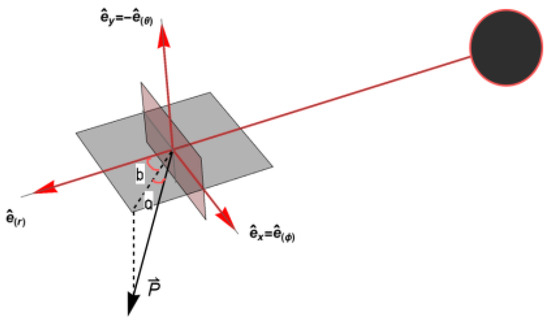
Figure 4.
The photon’s four-momentum projected onto the observer’s frame.
Here, represents the time-like vector whereas , and are the three basis vectors which correspond to the observer motion in the three spatial dimensions. The observer represented by the frame defined by (22) has zero angular momentum owing to the fact that . As a result, this observer is also referred to as the zero angular momentum observer.
The photon’s four momenta , when projected on the basis vector, result in directly measurable quantities in the observer’s local frame [12],
The observational angles a and b are then defined in terms of the four momenta as [12,13],
Considering that our observer is located at a distance from the black hole, then it is the apparent position in terms of Cartesian coordinates is expressed as [14],
Substituting the relations in Equation (24) as well as for from Equations (3)–(5) into Equation (25) gives
where
Furthermore, it is convenient to express these Cartesian coordinates in terms of and , which are the parameters depending on the constants of motion of the photons. Depending on the chosen values of and , the photons will occupy unique regions on the plane. For instance, when and are such that the photons follow spherical null geodesics, then the corresponding shape on the plane is a nearly circular image, which is the so-called critical curve. Besides, our goal is to conduct the ray-tracing analytically. It is then important that we have Equation (26) in terms of and since the equations of null geodesics depend on these two parameters instead of x and y. Thus, making and the subject in Equation (26) gives
Up to this point, we have the general expressions of the constants of motion in terms of the black-hole parameters, the observer position, and the Cartesian coordinates of the observer. It is important to note that these expressions are different from those derived in Equations (19) and (20). This is because Equations (19) and (20) defines only the special case when photons are bound at a constant radius while Equations (27) and (28) are general to any photon orbit.
To obtain the direct images, lensing rings, and photon rings, we will need to account for every turning point the photons make as they cross the equatorial plane. We consider photons crossing the equatorial plane as our approach is to obtain images of equatorial disks.
Thus, to achieve accurate analytic ray-tracing, it is crucial to present the solutions in terms of the turning points that photons undergo [13]. We then highlight the angular integrals in terms of the various turning points encountered by photons in the direction. This approach is enhanced by the establishment of definitions and signs that are beneficial for the analysis [15],
where m denotes the number of turning points. Furthermore, and denote the polar momentum at the endpoints and of the geodesic, respectively. Using the defined signs, the angular integrals unpack as [15],
Using Equation (29) alongside the general solutions in Equation (A15), we have
where . At this point, the relationship Equation (13) becomes important as we can now directly construct the images by applying the analytical expression
An investigation of the images of the equatorial disks for different values of m using the analytical expression Equation (31). This expression enables the separate investigation of different photon rings. Equation (31) provides a framework for visualizing rings based on the number of half-orbits, m, completed by a photon around the black hole. Additionally, it allows for the distinct visualization of rings associated with escape and plunge orbits. Moreover, Equation (31) offers a faster and more precise approach compared to computationally expensive numerical techniques, which often lack accuracy.
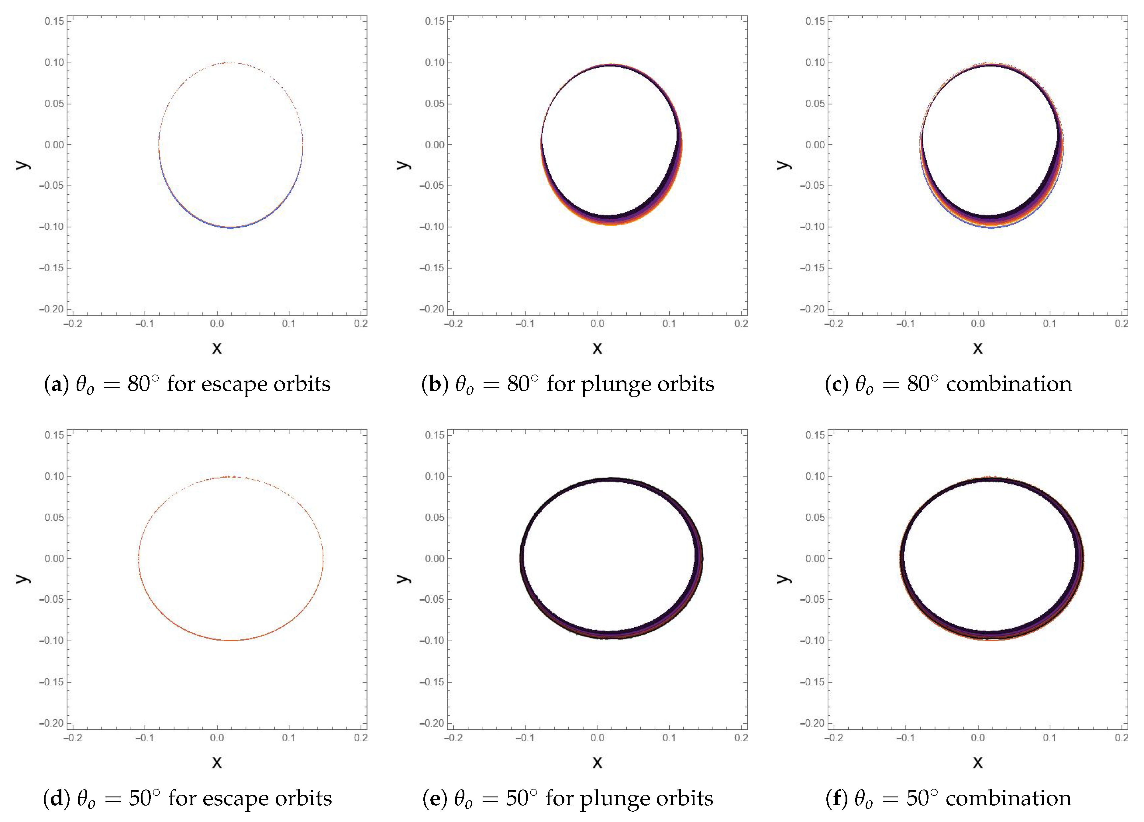
In Figure 5, we investigate the images for given two different angles of inclination, and . An observer detects these images after photons have crossed the equatorial disk once. The images for escape orbits are those images for which photons encounter a turning point in the exterior of a black hole and escape toward an observer. This region of the image forms the outer image while the region of the image for plunge orbits is that which arises from photons that do not encounter a turning point in the exterior of a black hole. As a result, these photons plunge into the black hole, forming the inner region on the observer’s screen. When the angle of inclination is lower, i.e., , the images appear to be nearly circular as compared to where they deviate so much from circularity. After just one half orbit, the orbits are weakly lensed; hence, the resulting images appear thick, as can be seen from the images in these plots.
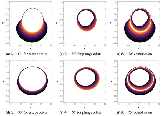
Figure 5.
Images of the equatorial disk for , , , for different angles of inclination of the observer.
In Figure 6, we investigate the images for for two different angles of inclination, and . An observer detects these images after photons have crossed the equatorial disk twice. When , the photons are on orbits that have undergone extreme lensing due to strong gravity. The resulting images appear extremely demagnified as compared to the images for which . Images for which comprises the photon ring. Since these images appear after photons have crossed the equatorial disk several times, their corresponding arrival time on the observer screen are different.
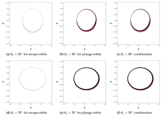
Figure 6.
Images of the equatorial disk for , , , for different angles of inclination of the observer.
4. Analysis of Critical Parameters
In this section, we will derive the relations for time delay, the Lyapunov exponent, and the change in azimuthal angle, which are the parameters governing the arrival time, demagnification, and rotation of subsequent images on the observer’s screen. Moreover, we will conduct an exploration of the influence of charge on these parameters as well as the cosmological constant. It is worth noting that subsequent images occur after photons make extra half-orbits around the black hole. Thus, for every extra half orbit a photon makes around the black hole, a different image that is exponentially demagnified appears on the observer’s screen. As a result, to express the critical parameters analytically, it is physically plausible to evaluate the angular integrals between two turning points, as this corresponds to half an orbit around the black hole.
4.1. Time Delay
Derivation of time delay will involve evaluation of Equation (9) over half an orbit. Solutions to the integrals over half-orbits have been expressed in Equations (A19)–(A21). As a result, Equation (9) becomes,
We note that the radial integral in Equation (9) has been expressed in terms of the angular integral through the relation Equation (13), resulting in the appearance of in the first term of Equation (32).
Figure 7 is an illustration of how varies with and . From the illustrations, it is clear that an increase in charge leads to a decrease in . For instance, when , we have that while when , we have that . Therefore, in a highly charged KNdS black hole, photons would take less time to complete half-orbits as compared to a less charged KNdS black hole. This then implies that subsequent images of a highly charged KNdS black hole will be detected faster by an observer. However, in the case of varying the cosmological constant, an increase in the value of results in an increase on . Thus, the implication of a larger cosmological constant would be that photons would take more time to complete half-orbits. This would then slow down the time of detection of subsequent images by an observer.
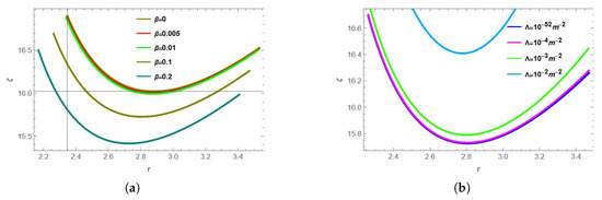
Figure 7.
Time delay for varying values of and . (a) Time delay for different values of with . (b) Time delay for different values of with .
Generally, in both cases, monotonically decreases to a minimum at a value of r, which corresponds to the radial position of the zero angular momentum orbit, before beginning to increase monotonically. As a result, when the black hole has spin, photons take different times to complete half-orbits depending on their radial position. In the case of spin zero (), no longer varies but rather takes specific values. This is owing to the fact that when black-hole spin is zero, the photon region reduces to a photon shell. Even so, as shown in Table 1, an increase in charge results in a decrease in the time taken for orbits to complete half-orbits, which corresponds to an observer detecting subsequent images faster when an RN black hole is highly charged. Moreover, an increase in the cosmological constant results in an increase in the time taken for photons to complete half-orbits. This implies that with a higher value of the cosmological constant, subsequent images of an RN black hole will be delayed more from being detected by an observer.

Table 1.
Time delay for varying values of , and spin zero ().
4.2. Lyapunov Exponent
The Lyapunov exponent, , gives the rate of exponential deviation of nearly bound orbits from the bound orbits. Denoting the radial coordinate of a bound photon as and considering a small deviation . Then, the radial coordinate of a nearly bound photon orbit will be . The next step is to perform a Taylor series expansion of the radial potential with respect to this deviation. This will result in
Equation (33) provides an approximation of a radial potential for a nearly bound photon orbit. We limit our consideration to terms up to the second order of as higher-order terms become extremely infinitesimal. Furthermore, , which is basically the condition for bound photon orbits. This condition implies that the first two terms of Equation (33) will vanish. By defining as the initial deviation and as the deviation after n half-orbits, then after n half-orbits, we show that
Simplifying Equation (34) results in,
Equation (35) gives the rate at which nearly bound photon orbits deviate from the bound photon orbits. This property gives rise to the exponential demagnification of the subsequent images of the photon ring.
As illustrated in Figure 8, an increase in charge results in a decrease in the rate of exponential deviation of nearly bound photons from bound photons. Thus, for a highly charged KNdS black hole, subsequent images will appear to be less demagnified as compared to the less charged KNdS black hole. Moreover, with the increasing value of the cosmological constant, the rate of exponential deviation also increases. This implies that with a higher value of , subsequent images will appear more demagnified as compared to smaller values of .
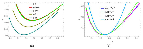
Figure 8.
Lyapunov exponent for varying values of , and . (a) Lyapunov exponent for different values of with . (b) Lyapunov exponent for different values of with .
Values of the Lyapunov exponent in the case of spin zero are as illustrated in Table 2. As shown, when the value of charge increases, the Lyapunov exponent decreases, implying that the rate of deviation of nearly bound photon orbits decreases. This corresponds to a decrease in the magnitude of demagnification of subsequent images. Similarly, an increase in the cosmological constant leads to a decrease in the Lyapunov exponent, indicating that a larger cosmological constant reduces the degree of demagnification of subsequent photon rings in a Reissner–Nordström–de Sitter black hole.
Table 2.
Lyapunov exponent for varying values of , and spin zero ().
4.3. Change in Azimuthal Angle
The change in azimuthal angle, , controls the rotation of subsequent images on the observer’s screen. This parameter is derived by evaluating Equation (8) over half-orbits. The solutions of the respective integrals evaluated over half-orbits have been given on Equations (A19)–(A21). Substituting these solutions into Equation (8) gives,
Equation (36) is the analytical expression with which to explore the amount of rotation subsequent images experience on the observer’s screen.
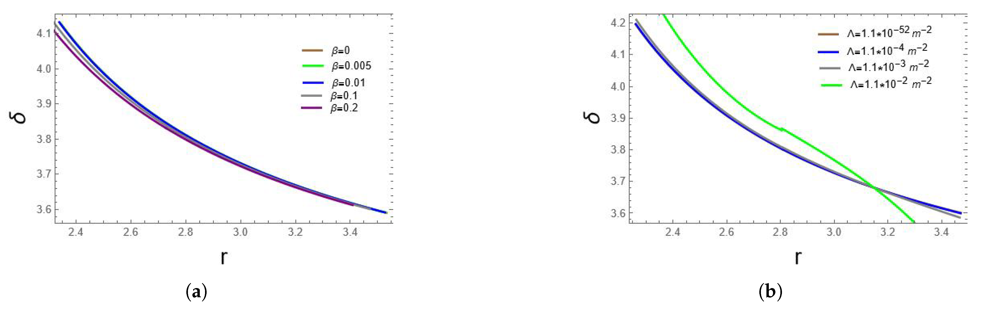
As illustrated Figure 9, the change in azimuthal angle is monotonic and indistinguishable for small values of cosmological constant. However, as increases or approaches , there is a considerable change implying that, for a KNdS black hole, an increase in leads to a greater change in azimuthal angle. For prograde orbits as , the change in azimuthal angle increases significantly and tends to decrease for retrograde orbits, i.e., beyond the . Furthermore, the change in azimuthal angle is also monotonic for different charge values. For prograde orbits, an increase in charge leads to a decrease in the change in azimuthal angle, as illustrated in the figure, whereas for retrograde orbits, the change in azimuthal angle for different values of charge is insignificant. From Table 3, in the case of spin zero, change in azimuthal angle does not vary with changes in charge but remains constant. This is brought about by the absence of frame-dragging for a non-rotating black hole making the change in azimuthal angle evolve symmetrically. On the other hand, an increase in leads to an increase in the change in azimuthal angle, though at a slow rate.

Figure 9.
Change in azimuthal angle for varying values of , and . (a) Change in azimuthal angle for different values of with . (b) Change in azimuthal angle for different values of with .
Table 3.
Change in azimuthal angle for varying values of , and spin zero ().
5. Conclusions
In this work, we have done an analytic investigation of the imprints of charge and LIVE on the photon ring of a KNdS black hole. Our analytic solutions of the integrals have made use of the Jacobi Elliptic integrals. We have analyzed images of equatorial disks for varying values of m, which we use to denote the number of times a photon crosses the equatorial plane. When , the photons are weakly lensed, and the images appear thick. However, as m increases, the photons are strongly lensed, which results in highly demagnified images referred to as the photon ring. Moreover, when , the images appear more circular for smaller angles of inclination, i.e., , and deviate extremely from circularity at higher observer inclination such as .
Imprints of charge on the critical parameters governing the exponential demagnification and arrival time of the subsequent images. These are the time delay , Lyapunov exponent , and change in azimuthal angle . We observe that an increase in charge leads to a decrease in the time delay. Therefore, in a highly charged KNdS black hole, photons would take less time to complete half-orbits as compared to a less charged KNdS black hole. This then implies that subsequent images of a highly charged KNdS black hole will be detected faster by an observer. However, in the case of varying the cosmological constant, an increase in the value of leads to an increase on . Thus, the implication of a larger cosmological constant would be that photons would take more time to complete half-orbits. This would then slow down the time of detection of subsequent images by an observer. Moreover, an increase in charge leads to a decrease in the rate of exponential deviation of nearly bound photons from bound photons. Thus, for a highly charged KNdS black hole, subsequent images will appear to be less demagnified as compared to the less charged KNdS black hole. Moreover, with the increasing value of the cosmological constant, the rate of exponential deviation also increases. This implies that with a higher value of , subsequent images will appear more demagnified as compared to smaller values of . Our conclusion for the imprints of charge is that the electromagnetic repulsion in the KNdS counteracts the gravitational attraction, and whereas the change in azimuthal angle is influenced mostly by the spin of the black hole, the charge has minimal effect on it. On the other hand, for the time delay and Lyapunov exponent, weaker gravitational attraction when the charge increases means that the photons will escape faster as compared to when the charge is less, hence stronger gravitational attraction. While a broader range of was explored for theoretical completeness, it is important to note that observational data suggest is on the order of .
Author Contributions
Conceptualization, J.M.; Software, D.W.; Formal analysis, J.M.; Investigation, J.M. and E.O.; Data curation, J.M.; Supervision, E.O.; Project administration, D.W. All authors have read and agreed to the published version of the manuscript.
Funding
This research received no external funding.
Data Availability Statement
The original contributions presented in the study are included in the article. Further inquiries can be directed to the corresponding author.
Conflicts of Interest
The authors declare no conflict of interest.
Abbreviations
The following abbreviations are used in this manuscript:
| LIVE | Lorentz Invariant Vacuum Energy |
| gr | General relativity |
| KdS | Kerr–de Sitter |
| KNdS | Kerr–Newman–de Sitter |
| EHT | Event Horizon Telescope |
| Sgr | Sagittarius |
Appendix A. Calculation of Roots of the Radial Potential
In this appendix, we illustrate Ferrari’s method with which we use to calculate the roots of the radial potential. In doing so, we express Equation (10) as,
The coefficients in (A1) have been defined as,
Given Equation (A1) is a quartic polynomial, Ferrari’s method gives the general form for its roots as,
In Equation (A3), is a root of the resolvent cubic of (A1) and can be obtained by first rewriting (A1) as,
A parameter p is introduced into (A4) by adding the terms on the left and right-hand side of Equation (A4) to obtain,
The right-hand side of (A5) is a perfect square, thus obtaining its discriminant and equating it to zero gives,
Equation (A6) is the resolvent cubic of Equation (A1) whose roots are obtained by first expressing it as a depressed cubic through the relation . This results in,
Cardano’s method gives the roots of (A7) where we select the real root,
We substitute v back into our relation for p to obtain
Finally, substituting (A9) into (A3) and distributing the signs results in the four roots of the radial potential,
Appendix B. Solutions to the Angular Integrals
In this section, we present the solutions of the angular integrals in terms of the Jacobi elliptic integrals of the first kind, second kind, and third kind. These integrals are, respectively, denoted as , , and . The angular potential is expressed in terms of its roots as:
where
Using this notation on the angular integrals results in,
Equation (A14), we have made use of the substitution while in Equation (A15) we have utilized . In the same approach, the solutions for the remaining integrals become,
The above integrals, when evaluated over half an orbit, i.e., performing integration over to or vice versa, reduce to
References
- Akiyama, K.; Alberdi, A.; Alef, W.; Asada, K.; Azulay, R.; Baczko, A.-K.; Ball, D.; Baloković, M.; Barrett, J.; Bintley, D.; et al. First M87 Event Horizon Telescope Results. I. The Shadow of the Supermassive Black Hole. Astrophys. J. Lett. 2019, 875, L1. [Google Scholar] [CrossRef]
- Akiyama, K.; Alberdi, A.; Alef, W.; Algaba, J.C.; Anantua, R.; Asada, K.; Azulay, R.; Bach, U.; Baczko, A.-K.; Ball, D.; et al. First Sagittarius A* Event Horizon Telescope Results. I. The Shadow of the Supermassive Black Hole in the Center of the Milky Way. Astrophys. J. Lett. 2022, 930, L12. [Google Scholar] [CrossRef]
- Johnson, M.D.; Akiyama, K.; Blackburn, L.; Bouman, K.L.; Broderick, A.E.; Cardoso, V.; Fender, R.P.; Fromm, C.M.; Galison, P.; Gómez, J.L.; et al. Key Science Goals for the Next-Generation Event Horizon Telescope. Galaxies 2023, 11, 61. [Google Scholar] [CrossRef]
- Akiyama, K.; Alberdi, A.; Alef, W.; Asada, K.; Azulay, R.; Baczko, A.-K.; Ball, D.; Baloković, M.; Barrett, J.; Bintley, D.; et al. First M87 Event Horizon Telescope Results. V. Physical Origin of the Asymmetric Ring. Astrophys. J. Lett. 2019, 875, L5. [Google Scholar] [CrossRef]
- Perlmutter, S.; Aldering, G.; Valle, M.D.; Deustua, S.; Ellis, R.S.; Fabbro, S.; Fruchter, A.; Goldhaber, G.; Groom, D.E.; Hook, I.M.; et al. Discovery of a supernova explosion at half the age of the Universe and its cosmological implications. Nature 1998, 391, 51–54. [Google Scholar] [CrossRef]
- Perlmutter, S.; Aldering, G.; Goldhaber, G.; Knop, R.A.; Nugent, P.; Castro, P.G.; Deustua, S.; Fabbro, S.; Goobar, A.; Groom, D.E.; et al. Measurements of Ω and Λ from 42 high redshift supernovae. Astrophys. J. 1999, 517, 565–586. [Google Scholar] [CrossRef]
- Garnier, A. Motion equations in a Kerr–Newman–de Sitter spacetime: Some methods of integration and application to black holes shadowing in Scilab. Class. Quantum Gravity 2023, 40, 135011. [Google Scholar] [CrossRef]
- Lupsasca, A.; Cárdenas-Avendaño, A.; Palumbo, D.C.; Johnson, M.D.; Gralla, S.E.; Marrone, D.P.; Galison, P.; Tiede, P.; Keeble, L. The Black Hole Explorer: Photon ring science, detection, and shape measurement. In Proceedings of the Space Telescopes and Instrumentation 2024: Optical, Infrared, and Millimeter Wave, Yokohama, Japan, 16–21 June 2024; SPIE: San Francisco, CA, USA, 2024; Volume 13092, pp. 2173–2197. [Google Scholar]
- Park, J.; Gwak, B. Bound on Lyapunov exponent in Kerr-Newman-de Sitter black holes by a charged particle. J. High Energy Phys. 2024, 2024, 23. [Google Scholar] [CrossRef]
- Gwak, B. Thermodynamics and cosmic censorship conjecture in Kerr–Newman–de Sitter black hole. Entropy 2018, 20, 855. [Google Scholar] [CrossRef]
- Slanỳ, P.; Stuchlík, Z. Equatorial circular orbits in Kerr–Newman–de Sitter spacetimes. Eur. Phys. J. C 2020, 80, 587. [Google Scholar] [CrossRef]
- Li, P.C.; Guo, M.; Chen, B. Shadow of a spinning black hole in an expanding universe. Phys. Rev. D 2020, 101, 084041. [Google Scholar] [CrossRef]
- Omwoyo, E.; Belich, H.; Fabris, J.C.; Velten, H. Black hole lensing in Kerr-de Sitter spacetimes. Eur. Phys. J. Plus 2023, 138, 1043. [Google Scholar] [CrossRef]
- Bardeen, J.M. Timelike and Null Geodesics in the Kerr Metric; Department of Physics Yale University: New Haven, CT, USA, 1973; pp. 215–240. [Google Scholar]
- Kapec, D.; Lupsasca, A. Particle motion near high-spin black holes. Class. Quantum Gravity 2019, 37, 015006. [Google Scholar] [CrossRef]


Disclaimer/Publisher’s Note: The statements, opinions and data contained in all publications are solely those of the individual author(s) and contributor(s) and not of MDPI and/or the editor(s). MDPI and/or the editor(s) disclaim responsibility for any injury to people or property resulting from any ideas, methods, instructions or products referred to in the content. |
© 2025 by the authors. Licensee MDPI, Basel, Switzerland. This article is an open access article distributed under the terms and conditions of the Creative Commons Attribution (CC BY) license (https://creativecommons.org/licenses/by/4.0/).