Existence in the Large for Caputo Fractional Multi-Order Systems with Initial Conditions

Abstract

One of the key applications of the Caputo fractional derivative is that the fractional order of the derivative can be utilized as a parameter to improve the mathematical model by comparing it to real data. To do so, we must first establish that the solution to the fractional dynamic equations exists and is unique on its interval of existence. The vast majority of existence and uniqueness results available in the literature, including Picard’s method, for ordinary and/or fractional dynamic equations will result in only local existence results. In this work, we generalize Picard’s method to obtain the existence and uniqueness of the solution of the nonlinear multi-order Caputo derivative system with initial conditions, on the interval where the solution is bounded. The challenge presented to establish our main result is in developing a generalized form of the Mittag–Leffler function that will cooperate with all the different fractional derivative orders involved in the multi-order nonlinear Caputo fractional differential system. In our work, we have developed the generalized Mittag–Leffler function that suffices to establish the generalized Picard’s method for the nonlinear multi-order system. As a result, we have obtained the existence and uniqueness of the nonlinear multi-order Caputo derivative system with initial conditions in the large. In short, the solution exists and is unique on the interval where the norm of the solution is bounded. The generalized Picard’s method we have developed is both a theoretical and a computational method of computing the unique solution on the interval of its existence.

1. Introduction

Fractional differential equations have various applications in widespread fields of science, such as engineering [1], chemistry [2,3,4], biology [5,6], physics [7,8,9], numerical analysis [10,11], and others [12,13]. In addition, Caputo fractional differential equations have the same initial and boundary conditions as the corresponding integer order dynamic equations. To use the order of the fractional derivative as a parameter to enhance the model, we need to show that the solution to the Caputo fractional differential equation exists and is unique on its interval of existence. However, a majority of the theoretical and computational methods of establishing existence and uniqueness results of dynamic equations are local existence results only. This includes Picard’s method as well, which is both a theoretical and a computational method of proving the existence and uniqueness results for dynamic equations with initial conditions. In this work, we generalize Picard’s method to provide an existence and uniqueness result in the large for the solution of the nonlinear multi-order Caputo differential system with initial conditions.

The incorporation of fractional derivatives of order $0<q<1$ allows for generalizations of the standard nonlinear system to multi-order systems where each iteration of the system has its own derivative order. A system of the form

$$\begin{array}{c}\hfill {}^{c}D^{0.65}{x}_1=f_1(t,x_1,x_2)\\ \hfill {}^{c}D^{0.75}{x}_2=f_2(t,x_1,x_2)\end{array}$$

would be a simple illustration of a multi-order system. However, the computation of the solution on its interval of existence is not guaranteed by Picard’s method. In [14], the authors have established that the fractional order of the derivative can be chosen as a parameter to enhance the model. With the modeling point in view, in this paper, we develop an existence result, namely existence in the large, for nonlinear multi-order fractional systems incorporating the Caputo fractional derivative with respect to time. In [15,16,17], the authors developed results for Riemann–Liouville multi-order systems. In their work, they constructed iterative techniques for various cases of multi-order systems, and their existence results were developed via upper and lower solution techniques. In [18], existence in the large was proven for the Caputo fractional reaction diffusion equation by Picard’s method. In [19,20], the authors studied two and three-order systems of Caputo fractional differential equations of the same fractional order derivative with initial conditions using the Laplace transform method.

In this paper, we establish that the solution to the nonlinear multi-order Caputo differential system exists and is unique on the entire time interval where the norm of the solution is bounded. This is what is referred to as existence in the large.

A common challenge when working with multi-order systems is that the generalized exponential function, also known as the Mittag–Leffler function, depends on the order of the derivatives in question. That is, ${}^{c}D^q{E}_q\left(\lambda t^q\right)=\lambda E_q\left(\lambda t^q\right)$ only if the order of the derivative and the parameter for the Mittag–Leffler function are equal. Overcoming this challenge requires the construction of a generalized form of the Mittag–Leffler function that will cooperate with all the fractional derivative orders in the system.

In Section 2, we recall known results of fractional differential equations. In Section 3, we establish a nice formula for the generalized Mittag–Leffler function which cooperates with all the different order derivatives of the system and proves its convergence is uniform, allowing term-by-term fractional calculus operations. In Section 3, we also prove the existence of a unique solution of the linear Caputo multi-order system and then develop a comparison theorem. This comparison theorem leads to a Gronwall-type inequality that we incorporate in the proof of our main result. Our main result is developed in Section 4, where we establish a generalized Picard’s existence and uniqueness result for the solution to the nonlinear Caputo multi-order system. Finally, we extend this result from a finite domain $[0,T]$ for any $T,$ $T<\infty$ where the solution of the system is bounded. It should be noted that in biological models, such as population models, the interval of existence is $[0,\infty ).$ On the other hand, the solution to $u^{\prime }=u^2,u\left(0\right)=1$ is known to exist on the interval $[0,1).$ However, the unique solution of ${}^{c}D^q=u^2,u\left(0\right)=1,$ cannot be computed easily. Using a comparison theorem, we can establish that the interval of existence for any $q<1$ is at best $[0,1-ϵ)$ for small $ϵ$, which depends on the value of $q.$ Here the value of q can be chosen in such a way that our solution matches realistic data. In Section 5, we develop illustrative numerical results for biological models, involving different-order Caputo fractional derivatives.

2. Preliminaries

In this paper, we examine existence and uniqueness results for multi-order systems of Caputo fractional differential equations of orders $0<q<1$ over the interval $J=[0,T]$. Our results employ the Caputo form of the fractional derivative given as

$${}^{c}D^{q}x\left(t\right)=\frac{1}{\Gamma (1-q)}{\int }_0^t{(t-s)}^{-q}\left(\frac{d}{ds}x\left(s\right)\right)ds,$$

for $x\in C^1\left(J\right)$. The corresponding fractional integral is defined as

$$I^{q}x\left(t\right)=\frac{1}{\Gamma \left(q\right)}{\int }_0^t{(t-s)}^{q-1}x\left(s\right)ds.$$

In this section, we recall results regarding the scalar nonlinear Caputo fractional initial value problem

$${}^{c}D^{q}x=f(t,x),x\left(0\right)=x_0,$$

(1)

with $t\in J$ and $x\in C^1\left(J\right)$. As seen in [12,21,22], if $x\in C^1\left(J\right)$, then (1) is equivalent to the fractional integral equation

$$x\left(t\right)=x_0+\frac{1}{\Gamma \left(q\right)}{\int }_0^t{(t-s)}^{q-1}f(s,x)ds.$$

An important function in the discourse of fractional calculus is the Mittag–Leffler function which, for parameters $\alpha ,\beta \in \mathbb{R}$, is defined as

$$E_{\alpha ,\beta }\left(\lambda t^q\right)=\sum _{k=0}^{\infty }\frac{{\left(\lambda t^q\right)}^k}{\Gamma (k\alpha +\beta )}$$

and is entire for $\alpha ,\beta >0$. The one-parameter Mittag–Leffler function defined as

$$E_{\alpha }\left(\lambda t^q\right)=E_{\alpha ,1}\left(\lambda t^q\right)=\sum _{k=0}^{\infty }\frac{{\left(\lambda t^q\right)}^k}{\Gamma (k\alpha +1)}$$

is a special case of the Mittag–Leffler function that is integral to the study of Caputo fractional derivatives, since ${}^{c}D^q{E}_q\left(\lambda t^q\right)=\lambda E_q\left(\lambda t^q\right)$. We refer the reader to [23] for more details.

Our results focus on the nonlinear multi-order N systems of the form

$${}^{c}D^{q_i}{x}_i=f_i(t,\mathit{x}),x_i\left(0\right)={\eta }_i.$$

(2)

where $0<q_i<1$, $\mathit{x}=(x_1,x_2,x_3,\dots ,x_N)$ and ${\eta }_i\in \mathbb{R}$ for each $i\in C=\{1,2,3,\dots ,N\}$. For simplicity, we will always assume i, or other indices, are in C unless stated otherwise. For convenience, we will be using the following notation

$${}^{c}D=({}^{c}D^{q_1},{}^{c}D^{q_2},{}^{c}D^{q_3},\dots ,{}^{c}D^{q_N}),\mathrm{and}\mathcal{I}=(I^{q_1},I^{q_2},I^{q_3},\dots ,I^{q_N}).$$

Thus, system (2) could be written as

$${}^{c}D\mathit{x}=\mathit{f}(t,\mathit{x}),\mathit{x}\left(0\right)=\mathbf{\eta },$$

where $\mathbf{\eta }=({\eta }_1,{\eta }_2,{\eta }_3,\dots ,{\eta }_N)$. The notation of multi-order integrals can be cumbersome, so let $K_i(t,s)=\frac{1}{\Gamma \left(q_i\right)}{(t-s)}^{q_i-1}$; additionally, we utilize $K_i$ when writing the Riemann–Liouville integral. Therefore, we can write ${\int }_0^t{K}_i(t,s)\varphi ds$ to mean the $q_i$ integral of any function $\varphi$. It should be noted that the Riemann–Liouville integral and the Caputo integral of the same order are the same.

In the next section, we develop a generalized Mittag–Leffler function and prove its uniform convergence and integral properties. From there, we establish a uniqueness result for a linear multi-order system and develop a Gronwall-style inequality for use in the proof of uniqueness in our main result for nonlinear systems.

3. Auxiliary Results

Results for the multi-order system involve a generalized Mittag–Leffler function. This function is an adjustment of the multi-order generalized exponential as discussed in [16]. Specifically, for $t\in J$ and a constant $\lambda \in \mathbb{R}$, we consider

$$Z(\lambda ,t)=\sum _{k_1=0}^{\infty }\sum _{k_2=0}^{\infty }\sum _{k_3=0}^{\infty }\cdots \sum _{k_N=0}^{\infty }\frac{\left({\lambda }^{k_1+k_2+\cdots k_N}\right)\left(t^{k_1{q}_1+k_2{q}_2+\cdots k_N{q}_N}\right)}{\Gamma (1+k_1{q}_1+k_2{q}_2+\cdots k_N{q}_N)}.$$

(3)

In [16], the functions constructed were generalizations of the two-parameter Mittag–Leffler function $E_{q_i,q_i}$, and they proved that the series converged uniformly. Thus, with only minor alterations, we can establish that Z converges uniformly on J as well. We show this proof next.

Theorem 1.

$Z(\lambda ,t)$ converges uniformly on J, and if $\lambda >0$, then for every i, $I^{q_i}Z(\lambda ,t)<\frac{1}{\lambda }Z(\lambda ,t)$ on J.

Proof. 

To begin the proof, we define $Z_i$ to be the first i sums of $Z(\lambda ,t)$; for example,

$$Z_3=\sum _{k_1=0}^{\infty }\sum _{k_2=0}^{\infty }\sum _{k_3=0}^{\infty }\frac{\left({\lambda }^{k_1+k_2+k_3}\right)\left(t^{k_1{q}_1+k_2{q}_2+k_3{q}_3}\right)}{\Gamma (1+k_1{q}_1+k_2{q}_2+k_3{q}_3)}.$$

Thus, with this notation, $Z_N=Z(\lambda ,t)$ and $Z_1=E_{q_1}\left(\lambda t^{q_1}\right)$, implying that $Z_1$ converges uniformly.

We will now prove that $Z_2$ converges uniformly. To do so, we utilize the beta function

$$B(x,y)={\int }_0^1{s}^{x-1}{(1-s)}^{y-1}ds$$

along with its decreasing nature. $B(x,y)$ decreases in x and y for $x,y>0$, since if $0<x_1\le x_2$, then for $s\in (0,1)$ we have $s^{x_1-1}\ge s^{x_2-1}$, implying $B(x_1,y)\ge B(x_2,y)$. The symmetry of B establishes its monotonicity in both variables.

Now, if we split off the $k_2=0$ term from $Z_2$, we are left with two series: one only in terms of $k_1$ and another in terms of both $k_1$ and $k_2$ with $k_2\ge 1$. The result is shown below:

$$Z_2=\sum _{k_1=0}^{\infty }\frac{{\lambda }^{k_1}{t}^{k_1{q}_1}}{\Gamma (1+k_1{q}_1)}+\sum _{k_1=0}^{\infty }\sum _{k_2=1}^{\infty }\frac{\left({\lambda }^{k_1+k_2}\right)\left(t^{k_1{q}_1+k_2{q}_2}\right)}{\Gamma (1+k_1{q}_1+k_2{q}_2)}.$$

The first term above is $Z_1$, which converges uniformly, so we will show that the double series above converges uniformly.

For $t\in J$ and every $k_1\ge 1,k_2\ge 0$, we have

$$\begin{array}{cc}\hfill \frac{\left({\lambda }^{k_1+k_2}\right)\left(t^{k_1{q}_1+k_2{q}_2}\right)}{\Gamma (1+k_1{q}_1+k_2{q}_2)}& \le B(1+k_1{q}_1,k_2{q}_2)\frac{\left({\lambda }^{k_1+k_2}\right)\left(T^{k_1{q}_1+k_2{q}_2}\right)}{\Gamma (1+k_1{q}_1)\Gamma \left(k_2{q}_2\right)}\hfill \\ \hfill & \le B(q_1,q_2)\frac{{\lambda }^{k_1}{T}^{k_1{q}_1}}{\Gamma \left(k_1{q}_1\right)}\frac{{\lambda }^{k_2}{T}^{k_2{q}_2}}{\Gamma (1+k_2{q}_2)}.\hfill \end{array}$$

(4)

Now we note that the second fraction in line (4) makes up the terms of $E_{q_2}\left(\lambda t^{q_2}\right).$ Next, we consider the first fraction, noting that

$$\sum _{k_1=1}^{\infty }\frac{{\lambda }^{k_1}{T}^{k_1{q}_1}}{\Gamma \left(k_1{q}_1\right)}=\sum _{k_1=0}^{\infty }\frac{{\lambda }^{k_1+1}{T}^{k_1{q}_1+q_1}}{\Gamma (k_1{q}_1+q_1)}=\lambda T^{q_1}{E}_{q_1,q_1}\left(\lambda T^{q_1}\right).$$

Applying these results and the Weierstrass M-test, we find that $Z_2$ converges uniformly on J.

The proof that the remaining $Z_i$ series converge uniformly follows by similar arguments. We show the details for $Z_3$, exemplifying how the later cases can be developed. We again start by isolating the $k_3=0$ term, yielding

$$Z_3=Z_2+\sum _{k_1=0}^{\infty }\sum _{k_2=0}^{\infty }\sum _{k_3=1}^{\infty }\frac{\left({\lambda }^{k_1+k_2+k_3}\right)\left(t^{k_1{q}_1+k_2{q}_2+k_3{q}_3}\right)}{\Gamma (1+k_1{q}_1+k_2{q}_2+k_3{q}_3)}.$$

As we just proved, $Z_2$ converges uniformly, so we focus on the triple series above. Thus, for $t\in J$, $k_1,k_2\ge 0$, and $k_3\ge 1$, we have

$$\begin{array}{cc}\hfill & \frac{\left({\lambda }^{k_1+k_2+k_3}\right)\left(t^{k_1{q}_1+k_2{q}_2+k_3{q}_3}\right)}{\Gamma (1+k_1{q}_1+k_2{q}_2+k_3{q}_3)}\hfill \\ \hfill & \le B(1+k_1{q}_1+k_2{q}_2,k_3{q}_3)\frac{\left({\lambda }^{k_1+k_2+k_3}\right)\left(T^{k_1{q}_1+k_2{q}_2+k_3{q}_3}\right)}{\Gamma (1+k_1{q}_1+k_2{q}_2)\Gamma \left(k_3{q}_3\right)}\hfill \\ \hfill & \le B(q_1+q_2,q_3)\frac{\left({\lambda }^{k_1+k_2}\right)\left(T^{k_1{q}_1+k_2{q}_2}\right)}{\Gamma (1+k_1{q}_1+k_2{q}_2)}\frac{{\lambda }^{q_3}{T}^{k_3{q}_3}}{\Gamma \left(k_3{q}_3\right)}.\hfill \end{array}$$

Similar to previous work, the first fraction makes up the terms of $Z_2$, and the second fraction makes up the terms of $\lambda T^{q_3}{E}_{q_3,q_3}\left(\lambda T^{q_3}\right)$. Therefore, by the Weierstrass M-test, $Z_3$ converges uniformly on J. Continuing this process, we can prove that every $Z_i$ converges uniformly, including the final step, which will give us that $Z_N$, that is $Z(\lambda ,t)$, converges uniformly on J. Since N is fixed and finite in this case, we can employ the above steps exhaustively; however, we can also inductively prove that $Z_N$ will converge uniformly for all N by utilizing the same steps.

Since convergence is uniform, we can take the fractional integral of the series term by term. To evaluate the fractional integral, we consider $i=1$ for simplicity and note that the same result will hold for every i.

$$\begin{array}{cc}\hfill I^{q_1}Z(d,t)& =\sum _{k_1=0}^{\infty }\sum _{k_2=0}^{\infty }\sum _{k_3=0}^{\infty }\cdots \sum _{k_N=0}^{\infty }\frac{\left({\lambda }^{k_1+k_2+\cdots k_N}\right)\left(t^{[k_1+1]q_1+k_2{q}_2+\cdots k_N{q}_N}\right)}{\Gamma (1+[k_1+1]q_1+k_2{q}_2+\cdots k_N{q}_N)}\hfill \\ \hfill & =\sum _{k_1=1}^{\infty }\sum _{k_2=0}^{\infty }\sum _{k_3=0}^{\infty }\cdots \sum _{k_N=0}^{\infty }\frac{\left({\lambda }^{[k_1-1]+k_2+\cdots k_N}\right)\left(t^{k_1{q}_1+k_2{q}_2+\cdots k_N{q}_N}\right)}{\Gamma (1+k_1{q}_1+k_2{q}_2+\cdots k_N{q}_N)}.\hfill \end{array}$$

(5)

Note that the sum in the second line of (5) is missing the $k_1=0$ term and, provided $\lambda >0$, this term will be positive. Further, since the calculation found in (5) will hold for all i, we can say that $I^{q_i}Z(\lambda ,t)<\frac{1}{\lambda }Z(\lambda ,t).$ □

Now we look at the homogeneous linear multi-order system with constant coefficients

$${}^{c}D\mathit{x}=A\mathit{x},\mathit{x}\left(0\right)=\mathbf{\eta },$$

(6)

where A is a real valued $N\times N$ matrix. Denoting the terms of $A=\left(a_{i,j}\right)$, we can equivalently write (6) as

$${}^{c}D^{q_i}{x}_i=\sum _{k=1}^N{a}_{i,k}{x}_k,x_i\left(0\right)={\eta }_i.$$

Many of our future results depend on the value of T from the interval $J=[0,T]$. To conveniently carry out these results, define $\tau$ as the constant

$$\tau =\left\{\begin{array}{cc}T& \mathrm{if}T\ge 1,\\ 1& \mathrm{if}T<1.\end{array}\right.$$

(7)

This constant is used frequently in our upcoming results, since $t^{q_i}\le \tau$ for all i, and $t\in J$ for any value of T.

In the following proof that the linear system has a unique solution, we utilize Caccioppoli’s extended Banach Contraction Mapping Principle, which we state below.

Theorem 2.

Let $(X,d)$ be a complete metric space, and let $f:X\to X$ be a mapping such that for each $n\ge 1$, there exists a constant $c_n$ such that

$$d(f^n\left(x\right),f^n\left(y\right))\le c_{n}d(x,y),$$

for all $x,y\in X$, where ${\sum }_{n=1}^{\infty }{c}_n<\infty$. Then, f has a unique fixed point.

We direct the reader to [24,25] for more details, including the proof. Now we will use this contraction mapping principle to prove that system (6) has a unique solution. Unless stated otherwise, we use the sum norm in our results, that is, $\parallel \mathit{x}\parallel ={\sum }_{i=1}^N\left|x_i\right|$.

Theorem 3.

The linear system (6) has a unique solution on J, and the successive approximations

$${\mathit{x}}_{n+1}={\mathit{x}}_0+\mathcal{I}\left(A{\mathit{x}}_n\right),{\mathit{x}}_0=\mathbf{\eta }$$

(8)

converge uniformly to the solution.

Proof. 

Let $\mathcal{J}\left(\mathit{x}\right)$ be the mapping

$${\mathcal{J}}_i\left(x_i\right)={\eta }_i+{\int }_0^t{K}_i(t,s)\sum _{k=1}^N{a}_{i,k}{x}_{k}ds.$$

For simplicity, let $M={max}_{i,j}\left|a_{i,j}\right|$, then

$$\begin{array}{cc}\hfill |{\mathcal{J}}_i\left(x_i\right)-{\mathcal{J}}_i\left(y_i\right)|& =\left|{\int }_0^t{K}_i(t,s)\sum _{k=1}^N{a}_{i,k}(x_k-y_k)ds\right|\hfill \\ \hfill & \le \frac{MN\parallel \mathit{x}-\mathit{y}\parallel }{\Gamma \left(q_i\right)}{\int }_0^t{(t-s)}^{q_i-1}ds\hfill \\ \hfill & =\frac{MN{t}^{q_i}}{\Gamma (q_i+1)}\parallel \mathit{x}-\mathit{y}\parallel \le \frac{MN\tau }{\Gamma (q_i+1)}\parallel \mathit{x}-\mathit{y}\parallel .\hfill \end{array}$$

Similarly,

$$\begin{array}{cc}\hfill & |{\mathcal{J}}_i^2\left(x_i\right)-{\mathcal{J}}_i^2\left(y_i\right)|\hfill \\ \hfill & =\left|{\int }_0^t{K}_i(t,s)\sum _{k=1}^N{a}_{i,k}\left({\mathcal{J}}_k\left(x_k\right)-{\mathcal{J}}_k\left(y_k\right)\right)ds\right|\hfill \\ \hfill & =\left|{\int }_0^t{K}_i(t,s)\sum _{k=1}^N{a}_{i,k}{\int }_0^s{K}_i(s,v)\sum _{k=1}^N{a}_{i,j}(x_j-y_j)dvds\right|\hfill \\ \hfill & \le M^2{N}^2\parallel \mathit{x}-\mathit{y}\parallel {\int }_0^t{K}_i(t,s)\left({\int }_0^s{K}_i(s,v)dv\right)ds\hfill \\ \hfill & =\frac{M^2{N}^2{t}^{2q_i}}{\Gamma (2q_i+1)}\parallel \mathit{x}-\mathit{y}\parallel \le \frac{M^2{N}^2{\tau }^2}{\Gamma (2q_i+1)}\parallel \mathit{x}-\mathit{y}\parallel .\hfill \end{array}$$

Continuing the process inductively, we can show that for all n,

$$|{\mathcal{J}}_i^n\left(x_i\right)-{\mathcal{J}}_i^n\left(y_i\right)|\le \frac{M^n{N}^n{\tau }^n}{\Gamma (n{q}_i+1)}\parallel \mathit{x}-\mathit{y}\parallel ,$$

therefore, for all n,

$$\parallel {\mathcal{J}}^n\left(\mathit{x}\right)-{\mathcal{J}}^n\left(\mathit{y}\right)\parallel \le \parallel \mathit{x}-\mathit{y}\parallel \sum _{k=1}^N\frac{M^n{N}^n{\tau }^n}{\Gamma (n{q}_k+1)},$$

and since $E_{q_i}\left(MN\tau \right)$ converges uniformly for every i, we obtain

$$\sum _{n=1}^{\infty }\sum _{k=1}^N\frac{M^n{N}^n{\tau }^n}{\Gamma (n{q}_k+1)}=\sum _{k=1}^N{E}_{q_k}\left(MN\tau \right).$$

Therefore, the mapping $\mathcal{J}$ has a unique fixed point by Theorem 2, implying (6) has a unique solution. □

The succeeding inequality properties help us prove uniqueness in our main result.

Corollary 1.

The solution to (6) satisfies the inequality

$$\parallel x\parallel \le \parallel \eta \parallel \left[1+2MN\tau \sum _{k=1}^N{E}_{q_k}\left(MN\tau \right)\right],$$

where $M={max}_{i,j}\left|a_{i,j}\right|.$

Proof. 

From Theorem 3, the sequence of successive approximations

$${\mathit{x}}_{n+1}=\mathcal{J}\left({\mathit{x}}_n\right)={\mathit{x}}_0+\mathcal{I}\left(A{\mathit{x}}_n\right),{\mathit{x}}_0=\mathbf{\eta }$$

converges uniformly, and since ${\mathit{x}}_n={\mathit{x}}_0+{\sum }_{k=1}^n({\mathit{x}}_k-{\mathit{x}}_{k-1})$ for all n, the series ${\sum }_{k=1}^{\infty }({\mathit{x}}_k-{\mathit{x}}_{k-1})$ also converges uniformly. Now, note from the previous proof we have

$$\begin{array}{c}\hfill \parallel {\mathit{x}}_2-{\mathit{x}}_1\parallel =\parallel \mathcal{J}\left({\mathit{x}}_1\right)-\mathcal{J}\left({\mathit{x}}_0\right)\parallel \le \parallel {\mathit{x}}_1-{\mathit{x}}_0\parallel \sum _{k=1}^N\frac{MN\tau }{\Gamma (q_k+1)}.\end{array}$$

Similarly,

$$\begin{array}{cc}\hfill \parallel {\mathit{x}}_3-{\mathit{x}}_2\parallel & =\parallel \mathcal{J}\left({\mathit{x}}_2\right)-\mathcal{J}\left({\mathit{x}}_1\right)\parallel =\parallel {\mathcal{J}}^2\left({\mathit{x}}_1\right)-{\mathcal{J}}^2\left({\mathit{x}}_0\right)\parallel \hfill \\ \hfill & \le \parallel {\mathit{x}}_1-{\mathit{x}}_0\parallel \sum _{k=1}^N\frac{M^2{N}^2{\tau }^2}{\Gamma (2q_k+1)};\hfill \end{array}$$

continuing this process inductively, we can show that

$$\parallel {\mathit{x}}_n-{\mathit{x}}_{n-1}\parallel \le \parallel {\mathit{x}}_1-{\mathit{x}}_0\parallel \sum _{k=1}^N\frac{M^n{N}^n{\tau }^n}{\Gamma (n{q}_k+1)}$$

for all n. Now let us consider $\parallel {\mathit{x}}_1-{\mathit{x}}_0\parallel$; for each i,

$$\begin{array}{cc}\hfill |{x_1}_i-{x_0}_i|& \le {\int }_0^t{K}_i(t,s)\sum _{k=1}^n\left|a_{i,k}{\eta }_k\right|ds\hfill \\ \hfill & \le N\parallel \eta \parallel \frac{M\tau }{\Gamma (q_i+1)}<2N\parallel \eta \parallel M\tau ,\hfill \end{array}$$

since $\frac{1}{\Gamma (q_i+1)}<2$ for each i. Thus, we have

$$\parallel {\mathit{x}}_1-{\mathit{x}}_0\parallel <2\parallel \eta \parallel NM\tau ,$$

leading to

$$\parallel {\mathit{x}}_n-{\mathit{x}}_{n-1}\parallel <2\parallel \eta \parallel MN\tau \sum _{k=1}^N\frac{M^n{N}^n{\tau }^n}{\Gamma (n{q}_k+1)}$$

for all n; since convergence is uniform, we have

$$\sum _{k=1}^{\infty }\parallel {\mathit{x}}_n-{\mathit{x}}_{n-1}\parallel \le 2\parallel \eta \parallel MN\tau \sum _{k=1}^N{E}_{q_k}\left(MN\tau \right).$$

This directly yields

$$\parallel \mathit{x}\parallel \le \parallel \eta \parallel \left[1+2MN\tau \sum _{k=1}^N{E}_{q_k}\left(MN\tau \right)\right],$$

which completes the proof. □

Remark 1.

We note that Corollary 1 implies that if $\mathbf{\eta }=\mathbf{0}$, then $\mathit{x}=\mathbf{0}$ on all of J.

Next, we develop a comparison theorem that provides conditions for when inequalities are preserved from original integral inequalities. This theorem is utilized in the uniqueness proof of our generalized Picard’s method.

Theorem 4.

Let $\mathit{y},\mathit{z}\in C^1\left(J\right)$ satisfy the inequalities

$$\begin{array}{cc}\hfill & \mathit{y}\ge \eta +\mathcal{I}\left(A\mathit{y}\right),\mathit{y}\left(0\right)\ge \mathbf{\eta },\hfill \end{array}$$

(9)

$$\begin{array}{cc}\hfill & \mathit{z}\le \eta +\mathcal{I}\left(A\mathit{z}\right),\mathit{z}\left(0\right)\le \mathbf{\eta },\hfill \end{array}$$

(10)

then $\mathit{z}\le \mathit{y}$ on J.

Proof. 

To begin, suppose the inequalities in (10) are strict inequalities; we show in this case that $\mathit{z}<\mathit{y}$. To prove this, suppose to the contrary that the set

$$\Lambda =\bigcup _{i=1}^N\{t\in J:y_i\left(t\right)\le z_i\left(t\right)\}$$

is non-empty. Let $\lambda =inf(\Lambda )$. Since $\mathit{z}\left(0\right)<\mathit{y}\left(0\right)$ and both are continuous over J, we can conclude that $z_i\left(\lambda \right)=y_i\left(\lambda \right)$ for some i and that $\lambda >0$. Therefore, since $\lambda$ is the infimum of $\Lambda$ and $\mathit{z}\le \mathit{y}$ on $[0,\lambda ]$, ${\sum }_{k=1}^N{a}_{ik}{z}_k\le {\sum }_{k=1}^N{a}_{ik}{y}_k$ on $[0,\lambda ].$ Then,

$$\begin{array}{cc}\hfill {\int }_0^{\lambda }{K}_i(\lambda ,s)\sum _{k=1}^N{a}_{ik}{z}_{k}ds& >z_i\left(\lambda \right)-{\eta }_i=y_i\left(\lambda \right)-{\eta }_i\hfill \\ \hfill & \ge {\int }_0^{\lambda }{K}_i(\lambda ,s)\sum _{k=1}^N{a}_{ik}{y}_{k}ds\hfill \\ \hfill & \ge {\int }_0^{\lambda }{K}_i(\lambda ,s)\sum _{k=1}^N{a}_{ik}{z}_{k}ds,\hfill \end{array}$$

which is a contradiction. Therefore, $\mathit{z}<\mathit{y}$ on J.

Now we will prove that $\mathit{z}\le \mathit{y}$ when the inequalities are not strict. Define the function ${\mathit{z}}_{\epsilon }$ for each i as ${z_{\epsilon }}_i=z_i-\epsilon \phi$, where $\phi =Z(2MN,t)$ as defined in (3). Then note that, since $\varphi \left(0\right)=1$, for each i,

$${z_{\epsilon }}_i\left(0\right)=z_i\left(0\right)-\epsilon <{\eta }_i.$$

Then for each i,

$$\begin{array}{cc}\hfill {z_{\epsilon }}_i-{\eta }_i+\epsilon \phi & \le {\int }_0^t{K}_i(t,s)\sum _{k=1}^N{a}_{i,k}{z}_{k}ds\hfill \\ \hfill & ={\int }_0^t{K}_i(t,s)\sum _{k=1}^N{a}_{i,k}\left[{z_{\epsilon }}_k+(z_k-{z_{\epsilon }}_k)\right]ds\hfill \\ \hfill & \le {\int }_0^t{K}_i(t,s)\sum _{k=1}^N\left[a_{i,k}{z_{\epsilon }}_k+M\epsilon \phi \right]ds\hfill \\ \hfill & <{\int }_0^t{K}_i(t,s)\sum _{k=1}^N{a}_{i,k}{z_{\epsilon }}_{k}ds+\frac{\epsilon \phi }{2}.\hfill \end{array}$$

The final inequality comes from Theorem 1, which implies $I^{q_i}\phi <\frac{1}{2MN}\phi$. This then implies that

$${z_{\epsilon }}_i<{\eta }_i+{\int }_0^t{K}_i(t,s)\sum _{k=1}^N{a}_{i,k}{z_{\epsilon }}_k.$$

Then by the previous case with strict inequalities, we have that ${\mathit{z}}_{\epsilon }<\mathit{y}$ on J. Then letting $\epsilon \to 0$, we obtain $\mathit{z}\le \mathit{y}$ on J. □

In the next section, we employ these results to prove existence in the large for system (2).

4. Main Result

What follows is a generalized Picard’s existence for system (2), which is then extended to existence in the large.

Theorem 5.

Assume $\mathit{f}$ is continuous on the rectangle S where

$$S=\left\{(t,x)|t\in [0,T],\parallel \mathit{x}\parallel <\infty \right\}$$

for some finite positive real number T. Further suppose $\mathit{f}$ attains the Lipschitz condition

$$|f_i(t,\mathit{x})-f_i(t,\mathit{y})|\le L\sum _{k=1}^N|x_k-y_k|$$

(11)

on S. Then (2) has a unique solution on $[0,T]$, and the successive approximations

$${\left(x_{n+1}\right)}_i={x_0}_i+{\int }_0^t{K}_i(t,s)f_i(t,{\mathit{x}}_n)ds,{x_0}_i={\eta }_i$$

(12)

exist on $[0,T]$ and converge uniformly to a solution x of (2).

Proof. 

First, we note that for all $n\ge 1$ we have

$${\mathit{x}}_n={\mathit{x}}_0+\sum _{k=1}^n({\mathit{x}}_k-{\mathit{x}}_{k-1}).$$

Therefore we utilize the Weierstrass M-test to show that the series ${\sum }_{k=1}^{\infty }({\mathit{x}}_k-{\mathit{x}}_{k-1})$ converges absolutely and uniformly, which in turn shows that $\left({\mathit{x}}_n\right)$ converges uniformly. The successive approximations described in (12) are defined on $[0,T]$, and since $\mathit{f}$ is continuous on S, there exists a positive constant M such that $\parallel \mathit{f}(t,{\mathit{x}}_0)\parallel \le M$ for all $t\in [0,T]$. Then note

$$\begin{array}{c}\hfill |{x_1}_i-{x_0}_i|\le \frac{1}{\Gamma \left(q_i\right)}{\int }_0^t{(t-s)}^{q_i-1}\parallel \mathit{f}(s,{\mathit{x}}_0)\parallel ds\le \frac{M{t}^{q_i}}{\Gamma (q_i+1)}\end{array}$$

for $t\in [0,T]$ and for all i. This implies that

$$\parallel {\mathit{x}}_1-{\mathit{x}}_0\parallel \le M\sum _{k=1}^N\frac{t^{q_k}}{\Gamma (q_k+1)}.$$

Then

$$\begin{array}{cc}\hfill |{x_2}_i-{x_1}_i|& \le \frac{1}{\Gamma \left(q_i\right)}{\int }_0^t{(t-s)}^{q_i-1}|f_i(s,{\mathit{x}}_{\mathbf{1}})-f_i(s,{\mathit{x}}_{\mathbf{0}})|ds\hfill \\ \hfill & \le \frac{L}{\Gamma \left(q_i\right)}{\int }_0^t{(t-s)}^{q_i-1}\parallel {\mathit{x}}_1-{\mathit{x}}_0\parallel ds\hfill \\ \hfill & \le \frac{ML}{\Gamma \left(q_i\right)}{\int }_0^t{(t-s)}^{q_i-1}\sum _{k=1}^N\frac{s^{q_k}}{\Gamma (q_k+1)}ds\hfill \\ \hfill & =ML\sum _{k=1}^N\frac{t^{q_k+q_i}}{\Gamma (q_k+q_i+1)}.\hfill \end{array}$$

Thus,

$$\parallel {\mathit{x}}_2-{\mathit{x}}_1\parallel \le ML\sum _{k_1=1}^N\sum _{k_2=1}^N\frac{t^{q_{k_1}+q_{k_2}}}{\Gamma (q_{k_1}+q_{k_2}+1)}.$$

For simplicity, let ${\sigma }_i=q_{k_i}$; continuing the previous process inductively, we can show

$$\begin{array}{cc}\hfill & \parallel {\mathit{x}}_n-{\mathit{x}}_{n-1}\parallel \hfill \\ & \le M{L}^{n-1}\sum _{k_1=1}^N\sum _{k_2=1}^N\sum _{k_3=1}^N\cdots \sum _{k_n=1}^N\frac{t^{{\sigma }_1+{\sigma }_2+\cdots {\sigma }_N}}{\Gamma (1+{\sigma }_1+{\sigma }_2+\cdots {\sigma }_n)}\hfill \\ \hfill & \le M{L}^{n-1}\sum _{k_1=1}^N\sum _{k_2=1}^N\sum _{k_3=1}^N\cdots \sum _{k_n=1}^N\frac{{\tau }^n}{\Gamma (1+{\sigma }_1+{\sigma }_2+\cdots {\sigma }_n)}\hfill \end{array}$$

(13)

for all $n\ge 2$, since $t^{{\sigma }_i}\le \tau$ for each i as defined in (7).

Now, in the direction of finding a bound on the above sums, let $\rho ={min}_{i\in C}\left\{q_i\right\}$ and note that $\frac{1}{\Gamma \left(z\right)}$ is decreasing for real numbers $z\ge 2$. Further note that there exists a $W>0$ such that $1+{\sum }_{i=1}^n{\sigma }_i\ge 2$ for all $n\ge W$. Therefore, we have that

$$\frac{1}{\Gamma \left(1+{\sum }_{i=1}^n{\sigma }_i\right)}\le \frac{1}{\Gamma (1+n\rho )},\mathrm{for}\mathrm{all}n\ge W.$$

Applying these results to the sums in (13), for $n\ge W$, we get

$$\begin{array}{cc}\hfill & \parallel {\mathit{x}}_n-{\mathit{x}}_{n-1}\parallel \le \frac{M{L}^{n-1}{N}^n{\tau }^n}{\Gamma (1+n\rho )}.\hfill \end{array}$$

The bounds above describe the terms of the convergent series $\frac{M}{L}{E}_{\rho }\left(LN\tau \right)$. Therefore, by the Weierstrass M-test, the series ${\sum }_{n=1}^{\infty }({\mathit{x}}_n-{\mathit{x}}_{n-1})$ converges absolutely and uniformly on $[0,T]$ and, in turn, ${\mathit{x}}_n$ converges uniformly on J. Therefore, letting $\mathit{x}=lim{\mathit{x}}_n$ and noting the convergence is uniform we obtain

$$\mathit{x}={\mathit{x}}_0+\mathcal{I}f(t,\mathit{x}),$$

implying this limit is a solution to (2). Now we wish to show this solution is unique, so let $\mathit{y}$ be another solution to (2), and let $\mathit{z}$ be defined as $z_i=|x_i-y_i|$ for each i. Now note that $\mathit{z}\left(0\right)=\mathbf{0}$ and

$$\begin{array}{cc}\hfill z_i& \le {\int }_0^t{K}_i(t,s)|f_i(t,\mathit{x})-f_i(t,\mathit{y})|ds\le {\int }_0^t{K}_i(t,s)L\sum _{k=1}^N{z}_{k}ds\hfill \end{array}$$

for each i. Now let $\hat{\mathit{x}}$ be the solution to the linear system

$${}^{c}D\hat{\mathit{x}}=\mathcal{L}\hat{\mathit{x}},\hat{\mathit{x}}\left(0\right)=\mathbf{0},$$

where $\mathcal{L}$ is the $N\times N$ matrix in which every entry is L. Then we have

$$\mathit{z}\le \mathcal{I}\left(\mathcal{L}\mathit{z}\right),\hat{\mathit{x}}=\mathcal{I}\left(\mathcal{L}\hat{\mathit{x}}\right),\mathrm{and}\mathit{z}\left(0\right)\le \hat{\mathit{x}}\left(0\right).$$

Then by Theorem 4, $\mathit{z}\le \hat{\mathit{x}}$; thus, by Remark 1, and since $\mathit{z}\ge 0$, we have that $\parallel \mathit{z}\parallel \le \parallel \hat{\mathit{x}}\parallel =0$, implying that the solution to (2) is unique. □

This result extends naturally to an existence in the large result given below. We note that we only extend this result to the positive t-axis due to the nature of fractional differential equations.

Theorem 6.

Assume $\mathit{f}$ is continuous and satisfies the Lipschitz condition (11) on each rectangle $S_{\lambda }$ for each λ where

$$S_{\lambda }=\left\{(t,\mathit{x})|t\in [0,\lambda ],\parallel x\parallel <\infty \right\}.$$

Then system (2) has a unique solution existing for all t.

This follows directly from the application of Theorem 5, as its hypotheses will be satisfied on each $S_{\lambda }$.

5. Applications

In this section we construct illustrative numerical examples of the generalized Picard’s method developed in Theorem 5. All computations and graph constructions were done with Python 3.9.6 on a 64-bit Windows 10 machine with a 3.4 GHz 6-core processor and 16 GB of RAM. We investigate the epidemic model studied in [20], first showing that the method applies to the single-order system and then expanding to illustrate the multi-order case.

The SIR model considered in this work was

$$\begin{array}{ccc}\hfill & {}^{c}D^{q}S\left(t\right)=-\beta S\left(t\right)I\left(t\right),\hfill & \hfill S\left(0\right)=L_1,\\ \hfill & {}^{c}D^{q}I\left(t\right)=\beta S\left(t\right)I\left(t\right)-\gamma I\left(t\right),\hfill & \hfill I\left(0\right)=L_2,\\ \hfill & {}^{c}D^{q}R\left(t\right)=\gamma I\left(t\right),\hfill & \hfill R\left(0\right)=L_3,\end{array}$$

where $\beta$ is the contact rate, and $\gamma$ is the recovery rate. $S\left(t\right)$ is the susceptible population, $I\left(t\right)$ is the infected population, and $R\left(t\right)$ is the population recovered from the disease. The authors assumed that the birth and death rates were the same for the small period of the epidemic. It is further assumed that there is no immigration and that the recovered population is immune to the disease, yielding a constant population. The authors of [20] utilized $\beta =0.01$, $\gamma =0.02$, $L_1=20$, $L_2=10$, and $L_3=5$ and examined values of $q\in \{0.8,0.85,0.9,0.95,1\}$. For the sake of comparison, we utilized the same values in our approximations. The numerical method employed computes the successive approximations from (8) up to ${\mathit{x}}_{99}$ with ${\mathit{x}}_0=(20,10,5).$

The graphs in Figure 1 show the numerical results of the generalized Picard’s method, and we find them reasonably close to results found in [20]. The computation speeds for these approximations averaged 7.762 s.

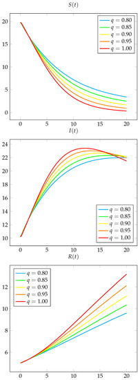
Figure 1. Solution curves for single-order systems.

For the second example, we extend the above system to the following multi-order system

$$\begin{array}{ccc}\hfill & {}^{c}D^{q_{\mathrm{1}}}S\left(t\right)=-\beta S\left(t\right)I\left(t\right),\hfill & \hfill S\left(0\right)=L_1,\\ \hfill & {}^{c}D^{q_{\mathrm{2}}}I\left(t\right)=\beta S\left(t\right)I\left(t\right)-\gamma I\left(t\right),\hfill & \hfill I\left(0\right)=L_2,\\ \hfill & {}^{c}D^{q_{\mathrm{3}}}R\left(t\right)=\gamma I\left(t\right),\hfill & \hfill R\left(0\right)=L_3,\end{array}$$

utilizing the same constants as before but now considering the following fractional derivative order groups

$$\begin{array}{ccccc}\hfill & Q_1=(0.8,0.7,0.8)\hfill & \hfill Q_2=(0.8,0.8,0.7)& \hfill & \hfill Q_3=(0.8,0.9,0.9)\\ \hfill & Q_4=(0.7,0.8,0.9)\hfill & \hfill Q_5=(0.7,0.9,0.8).\end{array}$$

These orders are chosen to illustrate the behavior of the multi-order case, which exemplifies how various orders can be chosen to better fit certain data. The approximations are computed in the same way as before, up to ${\mathit{x}}_{99}$. The computation time for the second example averaged 7.819 s. The results of the second example are shown in Figure 2.

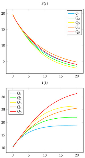
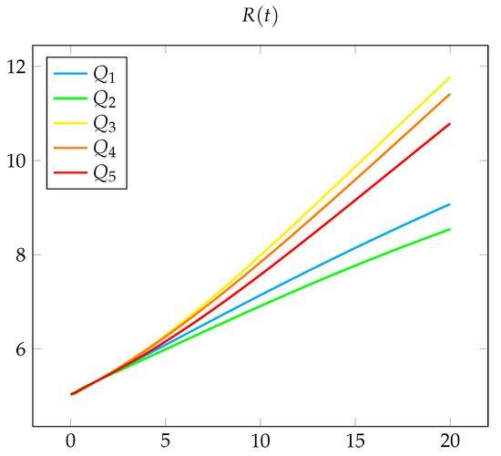
Figure 2. Solution curves for multi-order systems.

Concluding Remarks: In this work, we developed Picard’s method to prove the existence and uniqueness of the solution to multi-order Caputo systems with initial conditions. The advantage of the multi-order system is that the order of the derivatives can be used as a parameter to make the solution closer to the data available for any mathematical model compared with the integer order or Caputo fractional system of the same order. We note that if the goal is to find the best fit for the approximations, i.e., the ideal orders, then, unfortunately, this can only be done via trial and error at this time. Determining an analytic way to find the optimal order is still an open problem and something we wish to study in the future.

In [26,27], the authors studied sequential Caputo fractional differential equations and their applications. It should be noted that the solution to the sequential Caputo differential equations can be reduced to a Caputo fractional differential system. The Caputo fractional linear system with constant coefficients and initial conditions can be solved using the Laplace transform method. The explicit and numerical computation of the linear system is essential to solving the corresponding nonlinear system by any iterative method. We plan to explore the explicit and numerical computation of the Caputo multi-order linear system. This will pave the way to developing iterative methods to solve nonlinear systems combined with upper and lower solutions.

References

- Diethelm, K.; Freed, A. On the solution of nonlinear fractional differential equations used in the modeling of viscoplasticity. In Scientific Computing in Chemical Engineering II: Computational Fluid Dynamics, Reaction Engineering, and Molecular Properties; Keil, F., Mackens, W., Vob, H., Werther, J., Eds.; Springer: Berlin/Heidelberg, Germany, 1999; pp. 217–224. [Google Scholar]
- Glöckle, W.; Nonnenmacher, T. A fractional calculus approach to self similar protein dynamics. Biophy. J. 1995, 68, 46–53. [Google Scholar] [CrossRef] [PubMed]
- Metzler, R.; Schick, W.; Kilian, H.; Nonnenmacher, T. Relaxation in filled polymers: A fractional calculus approach. J. Chem. Phy. 1995, 103, 7180–7186. [Google Scholar] [CrossRef]
- Oldham, B.; Spanier, J. The Fractional Calculus; Academic Press: New York, NY, USA; London, UK, 2002. [Google Scholar]
- Zhou, Y.; He, J.W. A Cauchy problem for fractional evolution equations with Hilfer’s fractional derivative on semi-infinite interval. Fract. Calc. Appl. Anal. 2022, 25, 924–961. [Google Scholar] [CrossRef]
- Sivasankar, S.; Udhayakumar, R. Discussion on Existence of Mild Solutions for Hilfer Fractional Neutral Stochastic Evolution Equations Via Almost Sectorial Operators with Delay. Qual. Theory Dyn. Syst. 2023, 22, 67. [Google Scholar] [CrossRef]
- Sunthrayuth, P.; Shah, R.; Zidan, A.; Khan, S.; Kafle, J. The analysis of fractional-order Navier-Stokes model arising in the unsteady flow of a viscous fluid via Shehu transform. J. Funct. Spaces 2021, 2021, 1–15. [Google Scholar] [CrossRef]
- Aljahdaly, N.H.; Akgül, A.; Shah, R.; Mahariq, I.; Kafle, J. A comparative analysis of the fractional-order coupled Korteweg–De Vries equations with the Mittag–Leffler law. J. Math. 2022, 2022, 1–30. [Google Scholar] [CrossRef]
- Yang, W.; Wang, D.; Yang, L. A stable numerical method for space fractional Landau–Lifshitz equations. Appl. Math. Lett. 2016, 61, 149–155. [Google Scholar] [CrossRef]
- Sunthrayuth, P.; Ullah, R.; Khan, A.; Shah, R.; Kafle, J.; Mahariq, I.; Jarad, F. Numerical analysis of the fractional-order nonlinear system of Volterra integro-differential equations. J. Funct. Spaces 2021, 2021, 1–10. [Google Scholar] [CrossRef]
- Naeem, M.; Yasmin, H.; Shah, N.A.; Kafle, J.; Nonlaopon, K. Analytical Approaches for Approximate Solution of the Time-Fractional Coupled Schrödinger–KdV Equation. Symmetry 2022, 14, 2602. [Google Scholar] [CrossRef]
- Kilbas, A.; Srivastava, H.; Trujillo, J. Theory and Applications of Fractional Differential Equations; Elsevier: Amsterdam, The Netherlands, 2006. [Google Scholar]
- Kiryakova, V. Generalized Fractional Calculus and Applications; Pitman Research Notes in Mathematics Series; Longman-Wiley: New York, NY, USA, 1994; Volume 301. [Google Scholar]
- Almeida, R.; Bastos, N.R.O.; Monteiro, M.T.T. Modeling some real phenomena by fractional differential equations. Math. Methods Appl. Sci. 2016, 39, 4846–4855. [Google Scholar] [CrossRef]
- Denton, Z. Monotone method for multi-order 2-systems of Riemann-Liouville fractional differential equations. Commun. Appl. Anal. 2015, 19, 353–368. [Google Scholar]
- Denton, Z. Monotone Method for Riemann-Liouville Multi-Order Fractional Differential Systems. Opusc. Math. 2016, 36, 189–206. [Google Scholar] [CrossRef]
- Denton, Z.; Ramírez, J. Generalized Monotone Method for Multi-Order 2-Systems of Riemann-Liouville Fractional Differential Equations. Nonlinear Dyn. Syst. Theory 2016, 16, 246–259. [Google Scholar]
- Chhetri, P.; Vatsala, A. Existence of the Solution in the Large for Caputo Fractional Reaction Diffusion Equation by Picard’s Method. Dyn. Syst. Appl. 2018, 27, 837–851. [Google Scholar] [CrossRef]
- Pageni, G.; Vatsala, A.S. Study of two system of Caputo fractional differential equations with initial conditions via Laplace transform method. Neural Parallel Sci. Comput. 2021, 29, 69–83. [Google Scholar] [CrossRef]
- Pageni, G.; Vatsala, A. Study of Three Systems of Non-linear Caputo Fractional Differential Equations with Initial Conditions and Applications. Neural Parallel Sci. Comput. 2021, 29, 211–229. [Google Scholar] [CrossRef]
- Lakshmikantham, V.; Vatsala, A. Theory of fractional differential inequalities and Applications. Commun. Appl. Anal. 2007, 11, 395–402. [Google Scholar]
- Podlubny, I. Fractional Differential Equations; Academic Press: San Diego, CA, USA, 1999. [Google Scholar]
- Gorenflo, R.; Kilbas, A.A.; Mainardi, F.; Rogosin, S.V. Mittag-Leffler Functions, Related Topics and Applications; Springer: Berlin/Heidelberg, Germany, 2020. [Google Scholar]
- Almezel, S.; Ansari, Q.H.; Khamsi, M.A. Topics in Fixed Point Theory; Springer: Berlin/Heidelberg, Germany, 2014; Volume 5. [Google Scholar]
- Caccioppoli, R. Un teorema generale sull’esistenza di elementi uniti in una trasformazione funzionale. Rend. Accad. Naz. Lincei 1930, 11, 794–799. [Google Scholar]
- Vatsala, A.S.; Pageni, G.; Vijesh, V.A. Analysis of Sequential Caputo Fractional Differential Equations versus Non-Sequential Caputo Fractional Differential Equations with Applications. Foundations 2022, 2, 1129–1142. [Google Scholar] [CrossRef]
- Vatsala, A.; Pageni, G. Caputo Sequential Fractional Differential Equations with Applications. In Synergies in Analysis, Discrete Mathematics, Soft Computing and Modelling; Springer: Berlin/Heidelberg, Germany, 2023; pp. 83–102. [Google Scholar] [CrossRef]
Disclaimer/Publisher’s Note: The statements, opinions and data contained in all publications are solely those of the individual author(s) and contributor(s) and not of MDPI and/or the editor(s). MDPI and/or the editor(s) disclaim responsibility for any injury to people or property resulting from any ideas, methods, instructions or products referred to in the content. |
© 2023 by the authors. Licensee MDPI, Basel, Switzerland. This article is an open access article distributed under the terms and conditions of the Creative Commons Attribution (CC BY) license (https://creativecommons.org/licenses/by/4.0/).