Abstract
Computational fluid dynamics (CFD) is an effective technique to investigate atmospheric processes at a local scale. For example, in near-source atmospheric dispersion applications, the effects of meteorology, air pollutant sources, and buildings can be included. A prerequisite is to establish horizontally homogeneous atmospheric conditions, prior to the inclusion of pollutant sources and buildings. This work investigates the modelling of the atmospheric surface layer under neutral and stable boundary layer conditions, respectively. Steady-state numerical solutions of the Reynolds averaged Navier–Stokes (RANS) equations were used, including the k-ε turbulence model. Atmospheric profiles derived from the Cooperative Atmosphere-Surface Exchange Study-99 (CASES-99) were used as reference data. The results indicate that the observed profiles of velocity and potential temperature can be adequately reproduced using CFD, while turbulent kinetic energy showed less agreement with the observations under the stable conditions. The results are discussed in relation to the boundary conditions and sources, and the observational data.
1. Introduction
Computational fluid dynamics (CFD) is an effective technique to investigate atmospheric processes at a local scale. For example, in near-source atmospheric dispersion applications, the effects of meteorology, air pollutant sources, and buildings can be included. In order to investigate local processes in CFD, it is necessary to simulate an atmospheric surface layer. A prerequisite is to establish horizontally homogeneous atmospheric conditions, prior to the inclusion of pollutant sources and buildings.
Compared to neutral atmospheric conditions, a stable boundary layer (SBL) can suppress dispersion of emissions due to negative buoyancy effects, while an unstable boundary layer can enhance dispersion. This work investigates modelling of the atmospheric surface layer under neutral and SBL conditions, respectively.
It is a difficult process to model a realistic atmospheric boundary layer in CFD [1,2,3]. In addition, difficulties can arise due to unknown profiles of turbulence properties needed for modelling [4]. Under an SBL, shallow surface layers can occur, perhaps less than 10 m in depth, and it may be necessary to consider a much deeper layer. Several processes in the SBL can make this case much more difficult to investigate than neutral or unstable situations, including weak and intermittent turbulence, the production of elevated turbulence, and other phenomena [5,6,7].
The objective here was to attempt to establish a horizontally homogeneous atmospheric surface layer with the numerical model, whereby the inlet velocity and turbulence profiles, the ground shear-stress and turbulence model are in equilibrium. An approach for this under a neutral atmosphere is well established [1] and adopted here. An attempt is also made here to apply a similar approach to a SBL. For both neutral and stable atmospheres, the assumption was made that pressure was constant in the domain, and flow was driven by a shear stress at the top of the surface layer.
This paper is structured as follows. First, the CFD equations describing the situation are described. The numerical methods and the boundary conditions are then summarized. The CASES-99 data are described, as is the Monin–Obukhov similarity (MOS) theory which is used to provide profiles of velocity and temperature as upwind boundary conditions for CFD. Details of the approaches used to simulate both the neutral and the stable surface layers are given, followed by the results and discussion.
2. Materials and Methods
2.1. CFD Equations and Numerical Methods
A steady-state numerical solution has been used in CFD modelling of the surface layer [1,2,3,4]. For this work, the OpenFOAM steady-state solver for turbulent compressible flows was adapted, which includes solution of the conservation, momentum, turbulence, and enthalpy equations respectively [8]. Temperature is calculated from enthalpy using a numerical scheme [9]. The momentum and turbulence equations are given below, in order to show the specific terms used here.
The momentum conservation equation is given by [9]:
where u is the velocity vector; ρ is the density; p is the pressure; and μE is the sum of the molecular (μl) and turbulent viscosities (μt), respectively. The second term on the right-hand-side of Equation (1) is the buoyancy source term applied here, in which g = [0, 0, −9.8 m s−2]; ρ0 is the reference density at θ0(z), given by the lapse-rate of potential temperature. For neutral conditions, θ0 is constant. The rate of strain tensor D(u) is defined as: ).
The standard k-ε model was used to model turbulence [10]. k is the turbulent kinetic energy and ε is the turbulent dissipation rate:
where Pk is the volumetric production rate of k by shear forces; Gb is the volumetric production rate of k by buoyancy forces; σt,h is the turbulent Prandtl number (σt,h = 1.0, [11]); σk is the turbulent Prandtl number for k (σk = 1.0); σε is the turbulent Prandtl number for ε (σε = 1.31). The constants are: Cµ = 0.09, C1 = 1.44, C2 = 1.92. Gb is negative for stably stratified flows, so that k is reduced and turbulence is damped; while for unstably stratified flows, Gb is positive and k increases [12]. The coefficient C3 depends on the flow situation. In this work, a value of C3 = −0.8 was used [4].
OpenFoam uses the finite-volume method, whereby the terms in the conservation equations are discretized by integrating over the cell volume. The upwind-differencing scheme was used for the convective terms [13]. The discretized equations were solved using standard linear solver methods in OpenFoam. Pressure and velocities were coupled in the solution process using the SIMPLE algorithm [13]. The imbalances in the finite volume equation (the residuals) were used as a measure of the quality of the solution at each step in the iterative process. Iterations stop when the residual errors sum to less than user-set tolerances.
The key boundary conditions included: (i) upwind boundary: the appropriate vertical profiles of the relevant variables were set here, including velocity, potential temperature, k, and ε. (ii) downwind boundary: a fixed-pressure condition was applied, with an inlet-outlet condition for velocity. The inlet-outlet condition provides a zero-gradient condition for velocities, if outflow occurs, and fixed-value conditions on inflow. A fixed-pressure condition was applicable, since the variation of pressure due to hydrostatic effects was not included. (iii) ground surface: an atmospheric rough-wall function was applied. (iv) upper boundary: a fixed-pressure condition with an inlet-outlet condition for velocities was applied.
Simulations based on the finite volume method with flux defined boundary conditions (Neumann type) usually encounter numerical problems due to the backwards propagation of physical characteristics during the simulation procedure [4]. Fixed-temperature values (Dirichlet type) on both boundaries have been suggested as a compromise solution [4]. Fixed-temperature boundaries were used here at ground surface and at the upper-boundary, respectively. In a stably stratified condition, the heat flux is oriented downwards from upper to lower boundary and the value of the heat flux at the ground surface is negative.
2.2. CASES-99 Data
Near-surface profile data from CASES-99 [14] were used in this work. Data were obtained in netCDF format from EOS/NCAR [15]. The data were from the main CASES-99 60 m flux tower, and comprised 5-min averages of means, variances and covariances of the ISFF variables. Wind and temperature measurements on the 60 m tower were conducted by sonic anemometers at heights of 1.5, 5, 10, 20, 30, 40, 50, and 55 m [6]. This provided 3-component wind and temperature data at a sampling rate of 20 Hz. A number of low surface wind-speed situations were examined, and the profile data selected for the present work were from 18/10/1999 0900-0930 UTC, using a 30 min average. Wind-speed at a height of 1.5 m was 1.3 m/s, and a distinct temperature inversion existed. Wind and temperature profiles were found to be relatively steady over the course of the selected period. The virtual temperature profile data were adjusted by the dry adiabatic lapse-rate, to obtain potential temperature (θ) values. Dry air was assumed in the modelling. The roughness length used for the tower site was z0 = 0.03 m [16]. Wind vectors from the sonic anemometers were provided as rotated from instrument coordinates to normal meteorological coordinates. These data were converted to give the mean wind speed. Friction velocity ( = 0.12) and temperature scale ( = 0.07) were also needed for this work, and were obtained using the respective covariance values measured at the surface as follows [7]:
Turbulent kinetic energy (k) was obtained as:
2.3. MOS
It was attempted to reproduce the measured profiles of wind speed and θ using MOS flux-profile relationships [5]. The aim was to apply the MOS derived profiles as upwind boundary conditions. Flux-profile relationships relate the surface turbulent flux of momentum and heat to their respective profiles of mean wind speed and temperature [6]. When the turbulence covariances are not available, then turbulent fluxes of momentum and heat can be estimated from vertical profiles of mean values of wind speed and θ using MOS [2,17]. The MOS profiles of wind speed and θ are, respectively [5]:
where, ΨM = ΨT = 4.7 z/L; L is the Monin–Obukhov length; κ = 0.41 is the von Karman constant; u(z) is wind speed; θ(z) is the potential temperature; and θs is the surface temperature. For the case of neutral stability, only Equation (10) is relevant with ΨM = 0.
L is a measure of the height of the dynamical influence layer where surface properties are transmitted [7]. The surface layer height of a stable stratification is the same order as L [18]. For z > L, thermal influences are the dominant factor. In the present case, the value of L obtained was 14 m. Thus, the CASES-99 measurements taken at 20 m and above were not in the immediate surface layer, so may have been decoupled from surface influences to some extent. MOS assumes that the shear stress and heat flux are constant in the surface layer [2]. Reasonable agreements between MOS and the CASES-99 measurements were obtained, and this is presented below. The numerical simulations described next are an attempt to replicate the obtained MOS profiles of velocity and θ.
2.4. Experimental Procedure
The simulations were carried out in 2-D since the flow properties were invariant in the y-direction, but results were also confirmed in 3-D for selected cases. The test domain size was based on a scale suitable for near-surface dispersion modelling being 3000 m in length and 100 m in height. For the 3-D cases, a 40 m wide domain was used. The number of grid cells was: x (200), y (10), z (50), with gradation in the z-direction used to give greater resolution near the ground surface. The first cell center was located at a height of 0.15 m.
For the neutral case, the whole 100 m depth of the domain was contained in the surface layer, and the shear stress was assumed constant through the layer, equaling the shear stress at the surface. The approach taken for the neutral atmosphere applies analytic solutions to the momentum and turbulence equations as the upwind boundary conditions; and maintains a horizontally homogeneous atmosphere through the use of sources of momentum and ε applied at the upper boundary, and a rough wall function applied at the ground surface [1]. In order to satisfy the analytic solution, a different value of σε = 1.11 is used [1]. This approach ideally results in a logarithmic wind profile, a zero-vertical velocity, and constant values of k, θ, and pressure, respectively, everywhere in the domain. For the neutral case, the value of u* = 0.12 obtained above for the SBL, was used to provide the required value of u*, which determines the upwind profiles of wind speed, k, and epsilon [1]. This allowed both neutral and stable cases to be put on a common reference scale. However, u* reflects different relative magnitudes of mechanically- and buoyancy-driven turbulence in each atmosphere.
For the SBL case, the approach taken was similar, with the upwind boundary conditions given by MOS, and a rough wall function applied at the ground surface. However, two difficulties existed compared to the neutral case. First, with the surface layer depth of only 14 m, the way to model the situation was less clear. One possibility was to attempt to model only the lower 14 m or so in the SBL case. However, this would not be of much practical use in applications, where buildings are often higher than this, for example. The turbulent shear stress at the top of domain was not known, but the CASES-99 observation data indicated it may have been zero, since the observed shear stress fell from its surface value to zero at about 40 m. Thus, for the SBL, no source of momentum was applied at the upper boundary.
Second, known profiles for k and ε were not available for the SBL. If the measured profile of k was used, it was not sustained by the current model configuration which included the k-ε model, the boundary conditions, and numerical methods used. Thus, a different approach was taken in order to estimate the upwind boundary conditions for k and ε. The most consistent boundary conditions with respect to the applied equation system are the numerical results [4]. For a fixed bulk velocity, the turbulence characteristics can be obtained from the equilibrium state, as they result from the interaction of turbulent shear and inertial force [4]. Equilibrium profiles for k and ε were obtained here by running simulations on a domain 10 km in length, that is, beyond the distance where profiles were changing downwind.
3. Results
Figure 1 shows the results for the neutral atmosphere. It can be seen that the numerical results compare well with the analytic solutions for all variables. The velocity and θ profiles were maintained along the whole 3 km domain length. Although the analytic k profile was used as the upwind boundary condition, the k profile took some distance to stabilize to its equilibrium form but was sustained thereafter along the remaining length of the domain. Work is being aimed at better understanding this situation, including the initial values used and other numerical factors. The results indicated that the velocity and θ profiles were relatively insensitive to the specific form of the k profile. This may be because turbulence is a second order effect.
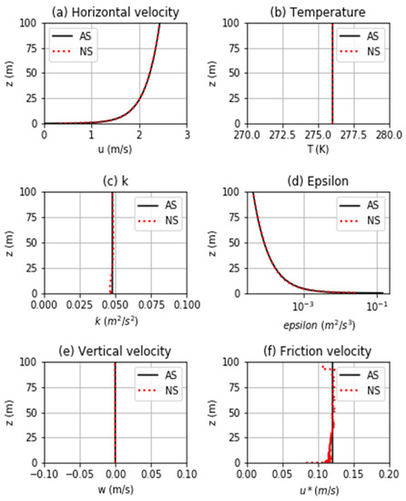
Figure 1.
Comparison of the numerical solution (NS) with the analytic solution (AS) for the neutral atmosphere. (a) horizontal velocity; (b) potential temperature; (c) turbulent kinetic energy; (d) turbulence dissipation rate; (e) vertical velocity; (f) friction velocity. The numerical results are shown for a position 2000 m from the upwind boundary of the domain.
Figure 2 shows the results for the SBL. It can be seen that reasonable agreement was found between the measured values of velocity and θ, and the respective profiles obtained from MOS; although the vertical structure of θ was more complex than the derived MOS profile. The numerical results compare well with the MOS profiles for horizontal velocity and θ in Figure 2a,b, respectively. In addition, k matches its reference profile reasonably well in Figure 2c. At equilibrium, turbulence production and destruction should be in balance, i.e., ε = Pk + Gb, and it can be seen in Figure 2f that the vertical profile of ε follows closely the production/destruction rates of k, indicating that equilibrium was attained. In summary, the numerical results were generally able to replicate the profiles derived from MOS based on the surface flux data.
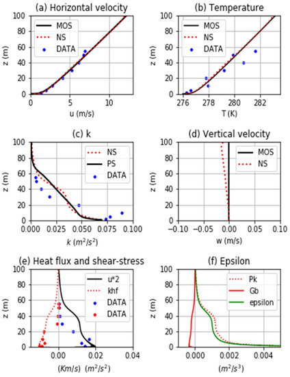
Figure 2.
Comparison of the numerical solution (NS) with the reference profiles for the stable atmosphere. (a) horizontal velocity; (b) potential temperature; (c) turbulent kinetic energy. PS refers to the precursor simulation result; (d) vertical velocity; (e) kinematic heat flux and shear-stress; (f) numerical production and dissipation of k. The numerical results are shown for a position 2000 m from the upwind boundary of the domain. Also shown are the CASES-99 data, where applicable.
4. Discussion
In contrast to the neutral case, it was found that the SBL profiles of horizontal velocity and k could be maintained without a shear stress applied to drive the flow at the top of the domain. The reason for this is not fully understood at this point, however a small negative vertical velocity was found in the solution in the top of the domain (Figure 2d), so air at the top velocity was being drawn into the domain through the upper boundary. This advection appears to be balancing the shear stress convergence in the lower part of the domain.
The numerical k profile is quite different compared to the CASES-99 measurements, being under-predicted below 20 m and over-predicted above this height (Figure 2c). It is not surprising that k does not capture the finer structure of the observations. No attempt was made to capture the specific detail of the observations at this stage. Indeed, such an attempt may be too ambitious using the current approach.
Figure 2e shows the modelled profiles of heat flux and shear stress, respectively. The CASES-99 observations of heat flux and shear stress are also shown. To some extent, a constant flux layer may be seen in the numerical results though it is deeper than the 14 m predicted by MOS, being around 40 m depth. This difference appears to be due mainly to the over-prediction of k centred at a height of around 40 m. Nevertheless, the result seems encouraging and suggests that, with further refinements to the current approach, it may be possible to model the depth and nature of the surface layer more accurately.
A number of factors are being considered that might lead to a better prediction of k. The observations indicate that θ increases with height at a greater rate than that predicted by the MOS-derived profile, as shown in Figure 2b. The magnitude of Gb may thus have been under-estimated, which could have led to greater modelled levels of k higher up in the domain than were measured. This is one aspect that will be tested in further work. Another factor being considered is the value used for C3, which affects the impact of the destruction rate in the k-ε model. Significant work has gone into optimizing the value of C3 [2]. Initial experiments in which different values of C3 were used have not yet shown any notable improvements in terms of results for k.
Acknowledgments
CASES-99 data provided by NCAR/EOL under the sponsorship of the National Science Foundation. https://data.eol.ucar.edu/ (accessed on 7 June 2021).
Conflicts of Interest
The author declares no conflict of interest.
References
- Richards, P.J.; Norris, S.E. Appropriate boundary conditions for computational wind engineering models revisited. J. Wind Eng. Ind. Aerodyn. 2011, 99, 257–266. [Google Scholar] [CrossRef]
- Alinot, C.; Masson, C. k-Epsilon model for the atmospheric boundary layer under various thermal stratifications. J. Sol. Energy Eng. 2005, 127, 438–443. [Google Scholar] [CrossRef]
- Yang, Y.; Gu, G.; Chen, S.; Jin, X. New inflow boundary conditions for modelling the neutral equilibrium atmospheric boundary layer in computational wind engineering. J. Wind Eng. Ind. Aerodyn. 2009, 97, 88–95. [Google Scholar] [CrossRef]
- Chang, C.-Y.; Schmidt, J.; Dorenkamper, M.; Stoevesandt, B. A consistent steady state simulation method for stratified atmospheric boundary layer flows. J. Wind Eng. Ind. Aerodyn. 2018, 172, 55–67. [Google Scholar] [CrossRef]
- Stull, R. An Introduction to Boundary Layer Meteorology; Springer: New York, NY, USA, 2009. [Google Scholar]
- Cheng, Y.; Oarlange, M.B.; Brutsaert, W. Pathology of Monin-Obukhov similarity in the stable boundary layer. J. Geophys. Res. 2005, 110, 1–10. [Google Scholar] [CrossRef]
- Yague, C.; Viana, S.; Maqueda, G.; Redondo, J.M. Influence of stability on the flux-profile relationships for wind speed, φm, and temperature, φh, for the stable atmospheric boundary layer. Nonlin. Process. Geophys. 2006, 13, 185–203. [Google Scholar] [CrossRef][Green Version]
- OpenFOAM. Available online: https://www.openfoam.com/ (accessed on 7 June 2021).
- Available online: http://caefn.com/openfoam/solvers-buoyantpimplefoam/ (accessed on 7 June 2021).
- Launder, B.E.; Spalding, D.B. The numerical computation of turbulent flows. Comput. Methods Appl. Mech. Eng. 1974, 3, 269–289. [Google Scholar] [CrossRef]
- Li, D. Turbulent Prandtl number in the atmospheric boundary layer—Where are we now? Atmos. Res. 2019, 216, 86–105. [Google Scholar] [CrossRef]
- CHAM. Available online: http://www.cham.co.uk/phoenics/d_polis/d_enc/turmod/enc_t341.htm/ (accessed on 7 June 2021).
- Versteeg, H.; Malalasekera, W. An. Introduction to Computational Fluid Dynamics: The Finite Volume Method; Pearson Education Limited: Essex, UK, 2007. [Google Scholar]
- Poulos, G.S.; Blumen, W.; Fritts, D.C.; Lundquist, J.K.; Sun, J.; Burns, S.P.; Nappo, C.; Banta, R.; Newsom, R.; Cuxart, J.; et al. CASES-99: A Comprehensive Investigation of the Stable Nocturnal Boundary Layer. Bull. Am. Meteor. Soc. 2002, 83, 555–581. [Google Scholar] [CrossRef]
- 5 Minute Statistics of ISFF Data during CASES-99 Version 1.0. 2016, UCAR/NCAR—Earth Observing Laboratory. Available online: https://www.eol.ucar.edu/field_projects/cases-99/ (accessed on 7 June 2021).
- Vickers, D.; Mahrt, L. The Cospectral Gap and Turbulent Flux Calculations. J. Atmos. Ocean. Technol. 2003, 20, 660–672. [Google Scholar] [CrossRef]
- Taylor, P.; Laroche, D.; Wang, Z.-Q.; McLaren, R. Obukhov Length Computation Using Simple Measurements from Weather Stations and AXYS Wind Sentinel Buoys; WWOSC: Montreal, QC, Canada, 2014. [Google Scholar]
- Emeis, S. Wind Energy Meteorology: Atmospheric Physics for Wind Power Generation; Springer Science & Business Media: New York, NY, USA, 2018. [Google Scholar]
Publisher’s Note: MDPI stays neutral with regard to jurisdictional claims in published maps and institutional affiliations. |
© 2021 by the author. Licensee MDPI, Basel, Switzerland. This article is an open access article distributed under the terms and conditions of the Creative Commons Attribution (CC BY) license (https://creativecommons.org/licenses/by/4.0/).