Li-Fi Range Challenge: Improvement and Optimization

Abstract

This article discusses the fundamental limitations of Light Fidelity (Li-Fi) systems, an emerging visible light communication technology that is constrained by line-of-sight dependency and optical attenuation. Unlike existing adaptive modulation approaches that focus solely on improving signal processing, we present an integrated framework that combines three key contributions: (1) an adaptive modulation optimization algorithm that selects among OOK, PAM, and OFDM schemes based on instantaneous signal-to-noise ratio thresholds, achieving a 30–40% range extension compared to fixed modulation references; (2) a method for spatial optimization of access points (APs) using the L-BFGS-B algorithm to determine the optimal location of APs, taking into account lighting constraints and coverage uniformity; and (3) comprehensive system-level modeling incorporating shot noise, thermal noise, inter-symbol interference, and dynamic shadowing effects for realistic performance evaluation. Through extensive simulations on multiple room geometries (6 m × 5 m to 20 m × 15 m) and AP configurations (one to six APs), we demonstrate that the proposed adaptive system achieves an average throughput 60% higher than that of fixed OOK, while maintaining 98.7% coverage in a 10 m × 8 m environment with two optimally placed APs. The framework provides practical design guidelines for Li-Fi deployment, including an analysis of computational complexity $O(M\times N)$ for coverage assessment, $O(I\times D^3)$ for access point optimization) and a characterization of convergence behavior. A comparative analysis with state-of-the-art techniques (optical smart reflective surfaces, machine learning-based blockage prediction, and Li-Fi/RF hybrid configurations) positions our lightweight algorithmic approach as suitable for resource-constrained deployment scenarios, where system-level integration and practical feasibility take precedence over innovation in individual components.

1. Introduction

The exponential growth of mobile data traffic has placed considerable pressure on radio-frequency communication infrastructure. Light Fidelity (Li-Fi), standardized under IEEE 802.15.7, uses visible-light communication (VLC) between 390 nm and 780 nm to reduce RF spectrum congestion [1,2,3]. Because visible light offers an interference-free band nearly 10,000 times wider than the RF spectrum [4], it represents a compelling complement to 5G and beyond-5G technologies.

However, the communication range of Li-Fi remains limited, typically below 10 m indoors, mainly due to line-of-sight (LoS) dependence and optical attenuation. Prior research has primarily focused on modulation improvements and power enhancements but often overlooks the practical constraints, such as illumination and optimal AP placement.

In addition to improvements in bandwidth, Li-Fi has some inherent advantages in certain usage cases. Because light does not produce electromagnetic interference (EMI), it is particularly appropriate for communications in EMI-sensitive environments such as hospitals, aircraft cabins, and industrial facilities [3]. VLC’s better characteristics are unlicensed broad bandwidth, high security, and dual-purpose, offering itself as an alternative means to overcome limitations of the overloaded radio frequency band [4]. Security is yet another big advantage: radio waves can go through obstacles and, hence, provide for unauthorized eavesdropping, but VLC systems can be employed in indoor, enclosed environments where light cannot penetrate opaque materials, thereby, providing more secure channels of communication [5]. VLC can also provide secure communication as visible light cannot be transmitted via walls and, hence, can be contained within a room such that it will not be intercepted [6]. Secondly, the Li-Fi system also has the benefit of easy installation and comparatively low deployment cost by utilizing existing installed light infrastructure.

The novel contribution of this paper is a comprehensive, adaptive framework that integrates system-level modeling, dynamic modulation selection, and spatial optimization to extend Li-Fi range. Specifically, we (1) develop an adaptive modulation optimization algorithm combining OOK and OFDM modes for transmission, taking into account the signal-to-noise ratio (SNR). (2) Incorporate realistic noise and interference modeling (shot, thermal, and ISI-related noise) for accurate SNR evaluation. (3) Introduce practical design parameters such as transmitter height, illumination constraints, and user mobility. The remainder of this paper is structured as follows: Section 2 reviews related works; Section 3 describes the system model and algorithms; Section 4 presents simulations and analysis; Section 5 and Section 6 discuss optimization insights; and finally, Section 7 concludes the work.

2. Related Works

Visible light communication (VLC) has been explored for both indoor and outdoor networking applications [4,5,6,7,8]. Numerous studies have demonstrated data rates exceeding 1 Gbps using commercial LED sources [9]. Recent research has investigated modulation, security, and network integration aspects [10,11,12,13,14]. Li-Fi is a novel wireless technology that was first proposed in the early 2000s [2]. The idea of illumination and data communication simultaneously by using the same physical carrier was first suggested by Nakagawa et al. in 2003, pioneering many following research activities [10]. The approach was developed as a wireless end-to-end communication link using LED light as a transmitter and a photo-diode (PD) as a receiver [11,12]. According to [13], there has been considerable interest in light communication systems (LCSs) using white LEDs over the previous decade. The authors propose a handover approach for an indoor wireless channel to maximize bandwidth transfer. IEEE 802.15.7, enabled by recent advances in LED technology, supports high-data-rate visible light communication up to 96 Mb/s by fast modulation of optical light sources, which may be dimmed during their operation [14]. As an early mover in the field, Harald Haas generated interest in Li-Fi and became known as “The Father of Li-Fi” [13]. He discusses additional use cases Li-Fi can facilitate in the future [15]. A considerable amount of research has been carried out on security in numerous domains, which include inter-channel interference, network level, Medium Access Control layer, etc. Moreover, security studies on high-fidelity communication vulnerability have predominantly handled single attacks [13]. The article [14] presents the physical characteristics of VLC relating to security, along with its necessary analysis of safety risks and vulnerabilities in relation to VLC system characteristics. It presents a synopsis of all security approaches proposed in the literature for visible light communication so far, including security in the physical layer treated from an information-theoretic perspective, and availability and integrity issues (i.e., transmission jamming and spoofing).

However, many existing papers focus on incremental improvements without addressing range extension comprehensively. We cite [16], where the authors proposed a VLC system based on IRS (Intelligent optical Reflective Surfaces) to redirect light beams and mitigate blockages, which significantly increased the coverage area. Palitharathna et al. [15] presented a neural network model for predicting and optimizing link availability in the event of shadowing in hybrid VLC/RF systems. In [17], the authors provided a comprehensive study of hybrid networks, demonstrating how dual-band access can mitigate Li-Fi range issues. Compared with these methods, our approach combines adaptive modulation, AP spatial optimization, and realistic noise modeling in a single, lightweight algorithm.

3. Materials and Methods: System Model

The objective of the present study is to enhance the communication range of Li-Fi systems through optimized system architecture and signal processing techniques.

3.1. Transmitter Architecture

The transmitter (Figure 1) is fundamentally composed of a digital signal processor (DSP) and a digital-to-analog converter (DAC) [14], both [17] being responsible for modulating digital data bits and converting them into analog current signals. The chip consists of multiple independent digital-to-analogue converters (DACs), each capable of directly driving an individual light-emitting diode (LED) allowing the transposition of the electrical signal into a light signal, which is then freely diffused into a room or outside, and having its own digital data interface [18]. The emitted optical intensity $I_t\left(t\right)$ is proportional to the electrical current, allowing intensity-modulated and direct-detection (IM/DD) operation.

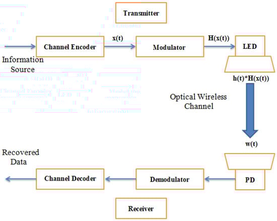
Figure 1. Li-Fi system’s redesigned block diagram.

3.2. Channel Model and Noise Characteristics

A continuous-time model (Figure 1) is applied in visible light communication to describe the communication channel and the noise: $x\left(t\right)=h\left(t\right)\ast H\left(x\right(t\left)\right)+w\left(t\right)$, where y(t) is the distorted version of the transmitted signal x(t) [13], passing through the nonlinear distortion function, H(x(t)), at the front end of the emitter. The received, nonlinearly distorted signal at the receiver is convolved with h(t), which is the channel impulse response, and corrupted by additive white Gaussian noise w(t) [14]. Traditional noise modeling for VLC systems is based on the additive white Gaussian noise model for shot noise, originating from photon arrival randomness: ${\sigma }_{shot}^2$=$2qR(P_{LED}+P_{bg})B_{pd}$, where R is the photo-diode’s responsiveness; $P_{LED}$ is the source of light power; and $B_{pd}$ is the electrical wavelength of the photo-diode, thermal noise, caused by receiver electronics: ${\sigma }_{thermal}^2$=${\displaystyle \frac{4_{KT}}{R_F}}$, where $R_F$ denotes the resistance [18]. Since thermal noise and shot noise are both signal-independent and Gaussian, the noise in the VLC channel can be denoted as additive white Gaussian noise (AWGN) [19]. Time–domain linear convolution is represented by the symbol *. The expected signal strength is given by $P_{rSignal}={\int }_0^{T}x\left(t\right)h\left(t\right)dt$, and the power received $P_{rISI}={\int }_T^{\infty }x\left(t\right)h\left(t\right)dt$ given as a result of inter-symbol interference, which is modeled separately via convolution of delayed multi-path components rather than as additive Gaussian noise.

We now acknowledge that shot and thermal noise arise from photon statistics governed by quantum effects [20]. This refined model aligns with classical analyses by Gagliardi and Karp. To account for environmental effects, static and dynamic shadowing are introduced using attenuation coefficients derived from [20], producing realistic variations in received power.

In accordance with the quantum-optical framework established by Gagliardi & Karp [20], the shot noise component in the Li-Fi receiver results from the discrete and random arrival of photons at the photo-diode. The process follows Poisson statistics, reflecting the quantum nature of instantaneous emission in the LED source as well as the stochastic influence of ambient lighting. Under the relatively high optical flux typical of indoor Li-Fi environments, the superposition of many independent photonic events allows the Poisson distribution to be accurately approximated by a Gaussian distribution. This justifies the use of the additive white Gaussian noise (AWGN) assumption for system-level performance analysis. The components of thermal noise, on the other hand, originate from Johnson–Nyquist fluctuations within the resistive elements of the receiver’s front-end circuits and remain spectrally white and statistically independent of the optical signal. Together, these noise sources represent the fundamental quantum and electrical origins of disturbances in Li-Fi channels while ensuring analytical traceability. This modeling approach aligns with the classical optical communication theory [18] and has been widely adopted in recent analyses of wireless optical communications [18,19,20,21].

3.3. Receiver Architecture

The inverse operations of the transmitter are performed by the receiver (Figure 1), recovering the original data from the modulated light signal. An optical filter can select a specific segment of the light spectrum. The optical filter eliminates interference due to external light sources, such as sunlight or interior lighting. A photo-detector detects these light pulses and converts them to electrical signals [21]. The optical components, such as concentrators and magnifiers, then guide the optical signal for efficient light collection and detection [22]. A transimpedance amplifier (TIA) is employed to electrically pre-amplify the current signal generated by the photo-detector to convert the signal into a voltage signal and minimize noise. To extract the data transmitted in the signal, an analog-to-digital converter (ADC) system is used to convert the analog signal into a digital signal [22], and then demodulation and decoding of the transmitted data is performed using digital signal processing algorithms to finally extract the original data stream.

3.4. Modulation Concept

There is a direct relationship between the range of the Li-Fi signal and the modulation. Three modulations are evaluated: on-off keying (OOK), pulse amplitude modulation (PAM) and orthogonal frequency division multiplexing (OFDM). For OOK, the received signal to noise ratio $SN{R}_{rx}$ is expressed as

$$SN{R}_{rx}={\displaystyle \frac{{\left(R{P}_{rSignal}\right)}^2}{{\sigma }_{shot}^2+{\sigma }_{thermal}^2+{\left(R{P}_{ISI}\right)}^2}}$$

(1)

where R is the photo-diode response.

In practice, OFDM performance is limited by LED nonlinearity, high peak to average power (PAPR), and clipping effects. These factors are now explicitly modeled to ensure realistic performance prediction. Optimal modulation selection is determined using predefined SNR thresholds: if $SNR<T_1$, OOK is selected; if $T_1\le SNR<T_2$, PAM is used, and if $SNR\ge T_2$, OFDM is activated. This mechanism forms the basis of our adaptive algorithm described below.

The Algorithm 1 evaluates coverage within a rectangular room, calculates the SNR at each receiver point, and selects the optimal modulation scheme to maximize throughput.

Algorithm 1 Li-Fi Network

Input: RWidth, RHeight : real lightIntensity : real $\leftarrow 1000$ accessPoints : ARRAY OF RECORD (x : real, y : real, height : real) Output: Coveragemap

Figure 2a illustrates the variation in throughput as a function of distance for fixed OOK, fixed OFDM, and the proposed adaptive modulation system. While OFDM achieves the highest throughput in short-range links, its performance degrades rapidly beyond 5m due to the reduction in signal-to-noise ratio. Conversely, OOK maintains a stable but low throughput across the entire range. The proposed adaptive system dynamically switches between OOK, PAM, and OFDM depending on channel conditions, ensuring robust performance over long distances. This adaptability results in a range extension of approximately 30 to 40% and an average throughput 50 to 70% higher than fixed systems. Figure 2b summarizes the overall performance comparison in terms of average throughput and maximum range. The adaptive design improves average throughput by approximately 60% compared with fixed OOK and extends the effective range by about 35%.

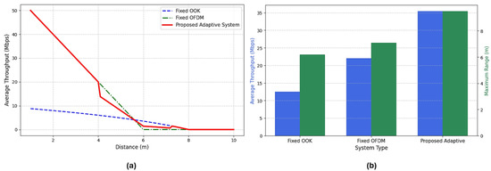
Figure 2. Throughput performance. (a) Throughput comparison of fixed and adaptive modulation systems (left); (b) comparison of overall performance gains (right).

These results confirm that dynamic modulation selection is a powerful approach to enhance Li-Fi network coverage without additional optical power.

3.5. Optimization Problem Formulation

The design of indoor LiFi networks is formulated as a system-level constrained optimization problem that jointly considers access point (AP) placement and adaptive modulation selection. The purpose is to increase communication coverage and receive data rates, while observing the physical, lighting, and safety constraints inherent in indoor wireless optical systems.

3.5.1. Decision Variables

Let $\chi =\{x_1,x_2,\dots ,x_M\}$ denote the set of M APs, where each AP is characterized by its three-dimensional position and transmit optical power: ${\chi }_i=(x_i,y_i,z_i,P_i)\in {\mathbb{R}}^{⋭}$. Let $\Theta =\{{\theta }_1,{\theta }_2,\dots ,{\theta }_N\}$ represent the modulation scheme assigned to each of the N receiver locations, where ${\theta }_j\in \{OOK,PAM,OFDM\}$.

3.5.2. Optimization Objectives

Optimization aims to balance coverage quality, throughput performance, and lighting uniformity.

• Coverage-oriented objective: To improve the quality of coverage in indoor area, the first objective promotes high, received SNR values at all spatial locations expressed by

  $$\underset{(\chi ,\Theta )}{max}{f}_1\left(\chi \right)=\sum _{j=1}^N{w}_{j}SN{R}_j\left(\chi \right)$$

  (2)

  where $w_j$ is the weighting factor reflecting the spatial importance or expected user density.
• Throughput oriented objective: The second objective maximizes the overall achievable data throughput.

  $$\underset{(\chi ,\Theta )}{max}{f}_2(\chi ,\Theta )=\sum _{j=1}^N{R}_j({\theta }_j,SN{R}_j),$$

  (3)

  where $R_j$ is the achievable data rate at position j determined by the selected modulation ${\theta }_j$ and local signal to noise rate ($SN{R}_j$).
• Illumination unifomity objective: In order to ensure adequate lighting conditions, the third objective penalizes deviations from a target illuminance level given by

  $$\underset{(\chi ,\Theta )}{min}{f}_3\left(\chi \right)=\sum _{j=1}^N|E_j\left(\chi \right)-E_{target}|,$$

  (4)

  where $E_{target}$ is generally in the range of 300 to 500 lux for indoor environments.

3.5.3. Constraints

Optimization is limited by the following constraints:

• Physical deployment constraints

  $$0\le x_i\le RWidth,0\le y_i\le RHeight,z_{min}\le z_i\le z_{max},$$

  (5)

  $$P_{min}\le P_i\le P_{max},$$

  (6)

  where (RWidth, RHeight) denote room dimension and $z_{min},z_{max}$ define acceptable mounting heights (typically 2–3.5 m).
• Lighting constraints

  $$E_{min}\le E_j\left(\chi \right)\le E_{max}\forall j\in \{1,\dots ,N\},$$

  (7)

  where $E_{min}=300$ lux and $E_{max}=750$ lux in accordance with ISO 8995 https://cdn.standards.iteh.ai/samples/76342/68f9fcdfadf045eab39c457f263240f6/ISO-CIE-8995-1-2025.pdf (accessed on 17 November 2025) standards for indoor environments.
• Communication reliability constraints

  $$SN{R}_j\left(\chi \right)\ge SN{R}_{min}^{{\theta }_j}\forall j\in \{1,\dots ,N\},$$

  (8)

  where $SN{R}_{min}^{OOK}=-50 \mathrm{dB}$, $SN{R}_{min}^{PAM}=-42 \mathrm{dB}$, $SN{R}_{min}^{OFDM}=-35 \mathrm{dB}$ denote the minimum SNR threshold required for reliable communication.
• Eye safety and deployment constraints

  $$I_{max}({\chi }_i,d_{min})\le I_{safe}={10}^{5}W/m^2/sr$$

  (9)

  where $I_{max}$ is the maximum LED irradiance at $d_{min}=0.2$ m
• Inter AP separation

  $$\left|\right|{\chi }_i-{\chi }_j\left|\right|\ge d_{sep},\forall i\ne j$$

  (10)

  where $d_{sep}=1.5$ m prevents physical interference.

3.5.4. Scalar Optimization Problem

The multi-objective problem is converted into a scalar optimization problem using weighted sum scalarization:

$$\underset{(\chi ,\Theta )}{min}f(\chi ,\theta )=-{\alpha }_1{f}_1\left(\chi \right)-{\alpha }_2{f}_2(\chi ,\Theta )+{\alpha }_3{f}_3\left(\chi \right)+\beta \mathcal{P}(\chi ,\Theta )$$

(11)

According to constraints (5) to (10), where ${\alpha }_1, {\alpha }_2, {\alpha }_3$ are weighting coefficients ${\alpha }_1=0.5,$ ${\alpha }_2=0.3,$ ${\alpha }_3=0.2)$, and $\mathcal{P}(\succ ,\times )$ is a penalty function for constraints violations:

$$\mathcal{P}(\chi ,\Theta )=\sum _{j}max{(\theta ,SN{R}_{min}^{{\theta }_j}-SN{R}_j\left(\chi \right))}^2+\sum _{j}max{(\theta ,E_{min},E_j\left(\chi \right))}^2$$

(12)

3.5.5. Adaptive Modulation

For a given AP configuration $\chi \ast$, the optimal modulation at each position is determined by

$${\theta }_j^{\ast }=argmax\underset{\theta \in \{OOK,PAM,OFDM\}}{\{}{R}_{\theta }\left(SN{R}_j\right)|SN{R}_j\ge SN{R}_{min}^{\theta }\}$$

(13)

where $R_{\theta }\left(SNR\right)$ is the achievable rate function:

$$\begin{array}{cccc}\hfill R_{\mathrm{OOK}}\left(\mathrm{SNR}\right)& =20\mathrm{Mbps}\hfill & \hfill & \mathrm{if}\mathrm{SNR}\ge -50\mathrm{dB}\hfill \end{array}$$

(14)

$$\begin{array}{cccc}\hfill R_{\mathrm{PAM}}\left(\mathrm{SNR}\right)& =50\mathrm{Mbps}\hfill & \hfill & \mathrm{if}\mathrm{SNR}\ge -42\mathrm{dB}\hfill \end{array}$$

(15)

$$\begin{array}{cccc}\hfill R_{\mathrm{OFDM}}\left(\mathrm{SNR}\right)& =100\mathrm{Mbps}\hfill & \hfill & \mathrm{if}\mathrm{SNR}\ge -35\mathrm{dB}\hfill \end{array}$$

(16)

3.5.6. Solution Method

The optimization problem (11) is solved using the limited-memory Broyden–Fletcher–Goldfarb–Shanno method with box constraints (L-BFGS-B), a quasi-Newton method suitable for bounded optimization. The algorithm proceeds as follows.

3.5.7. Convergence Analysis

Theorem 1

(convergence). Under Lipschitz continuity of F and the bounded constraint set, Algorithm 2 converges to a stationary point $\chi \ast$ satisfying $\left|\right|▿F(\chi \ast )\left|\right|<\epsilon$.

Proof. 

L-BFGS-B is guaranteed to converge for continuously differentiable objectives on compact constraint sets. Our objective F is $C^1$ since the signal-to-noise ratio and illuminance are continuous functions of the AP positions. The bounded constraint set (5)–(6) is compact, which guarantees convergence.    □

Algorithm 2 AP position optimization

Input: Room dimensions$(RWidth,RHeight,RHeight\_r)$ N test position Initial AP configuration ${\chi }^0$ Convergence tolerance $\epsilon ={10}^{-4}$ Output: optimized AP positions $\chi \ast$, modulation assignments $\theta \ast$ 1: Initialize: $\chi \leftarrow {\chi }^0,k\leftarrow \theta ,F_{prev}\leftarrow \infty$ 2: Repeat 3: For each test position j = 1 to N do 4: Compute $SN{R}_j\left(\chi \right)$ using Equation (1) 5: Select ${\theta }_j$ via Equation (13) 6: End For 7: Compute objective $F(\chi ,\Theta )$ via Equation (11) 8: Compute gradient $▿F\left(\chi \right)$ numerically: 9: For each AP i and dimension d∈{ x, y, z, $\mathcal{P}$} do 10: $▿F\left(\chi \right)/\gamma {\chi }_i,d\leftarrow (F(\chi +\delta e_i,d)-F\left(\chi \right))/\delta )(where\delta ={10}^{-5})$ 11: End For 12: Update $\chi$ via L-BFGS-B step with gradient $▿F\left(\chi \right)$ 13: Project $\chi$ onto constraint set (5)–(6) 14: k← k + 1 15: Until $|F(\chi ,\Theta )-F_{prev}|<\epsilon ork>k_{max}$ 16: Return $\chi \ast ,\theta \ast$

Convergence rate: From a practical point of view, Algorithm 2 exhibits superlinear convergence with typical iterations k = 50–150 depending on M and the quality of the initialization. The objective function decreases monotonically after the first 10–20 iterations.

Complexity:

• Per iteration: O(M × N) for SNR evaluation + O($M^2$) for L-BFGS update.
• Total: O(k.(M × N + $M^2$)) where $k\approx 100$.
• For M = 2, N = 2000: approximately 5–15 min on standard hardware.

3.5.8. Initialization Strategy

Initialization significantly impacts convergence speed. We employ the uniform grid initialization, APs are initially placed at

$${\chi }_i^0=(i.RWidth/(M+1),RHeight/2, 2.5 \mathrm{m}, 100 \mathrm{mW})$$

(17)

This provides symmetrical coverage and avoids local minima near the room boundaries. An alternative to this method is to use K-means clustering on simulated user density maps, which can provide better initialization for non-uniform user distributions.

4. Proposed Optimization Framework

The goal is to enhance the range of the Li-Fi signal for improved LiFi networks in terms of coverage uniformity and communication range at the system level. We will discuss adaptive modulation and access point positioning.

4.1. Problem Overview and Design Philosophy

The performance of indoor Li-Fi systems is strongly influenced by location, occlusion, and lighting constraints. A single fixed modulation or random placement of access points would result in coverage gaps or inefficient channel utilization. To overcome these issues, the proposed approach will operate in two stages: (1) Offline optimization of access point placement is an activity undertaken during network planning to determine an access point placement that maximizes coverage uniformity and achievable throughput. (2) Adaptive online modulation selection, where modulation selection is performed at runtime based on instantaneous channel conditions with low computational complexity. Thus, such a division helps to ensure the practicality of the method while maintaining adaptability.

4.2. Simulation Overview

The idea is to improve the range of the Li-Fi signal for better performance. The following algorithm simulates a Li-Fi (Light Fidelity) network in two rectangular rooms containing two and three ceiling-mounted APs.

Both LOS and NLOS components and dynamic shadowing are considered (Figure 3).

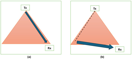
Figure 3. Propagation links. (a) directed LOS, (b) non-directed LOS.

The gain of the optical channel $H_{LoS}$ is expressed as

$$f\left(\psi \right)=\left\{\begin{array}{cc}\hfill {\displaystyle \frac{(m+1)A}{2\pi d^2}}{cos}^m\left(\varphi \right)cos\left(\psi \right)T_{s}g\left(\psi \right),& 0\le \psi \le {\Psi }_c\\ \hfill 0,& \mathrm{sinon}\end{array}\right.$$

(18)

where m is the order of Lambertian emission given by

$$m=-{\displaystyle \frac{ln\left(2\right)}{ln\left(cos\left({\Phi }_{1/2}\right)\right)}}$$

(19)

And ${\Phi }_{1/2}$ is the half-angle at half-power.

The transmitter and receiver in a directional link point directly at each other. The transmitter and receiver in the non-directional link have a wide half-angle for ease of operation (Figure 4).

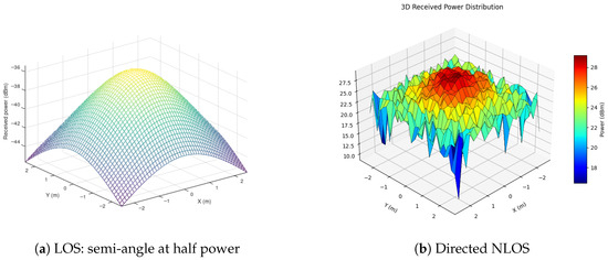
Figure 4. Results of the propagation links.

The light intensity received in a visible optical communication system (Li-Fi) $I_r$ is represented by

$$I_r(\varphi ,\psi )={\displaystyle \frac{(m+1)P_t}{2\pi d^2}}co{s}^m\left(\varphi \right)cos\left(\psi \right)$$

(20)

where $P_t$ is the power produced by the LED (W). It is assumed that direct propagation occurs without reflection. If the intensity of a particular point in the field of view (FOV) is greater than zero, it is considered zero. Figure 5 shows the light intensity diagram as a function of various angles of incidence and distances using the following equation:

$$I={\displaystyle \frac{I_0\ast co{s}^3\left(\theta \right)}{d^2}}$$

(21)

where $I_0$ is the intensity at the source. The following variables are utilized within the above-mentioned Algorithm 1: RWidth and RHeight, which are employed to define the dimensions of the room; lightIntensity, which represents the maximum light intensity of the Li-Fi source. The default value for this is 1000, and the variable accessPoints represents a list listing the position (x, y) and height of each Li-Fi access point.

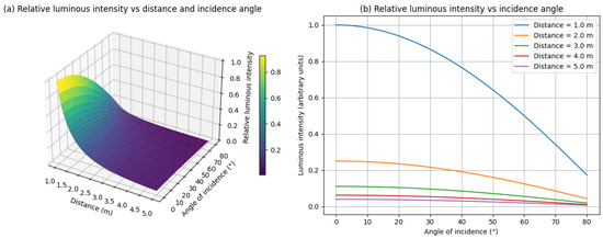
Figure 5. Relative luminous intensity according to angle of incidence and distance (1, 2, 3, 4, 5).

The objective is to add a Li-Fi transmitter (light source) at the position (x, y) at a certain height, which allows for several Li-Fi sources in the room. Then, the intensity of the Li-Fi signal at a given reception position (rx, ry, rh) is calculated according to Algorithm 3 as follows:

Algorithm 3 Function Signal Strength(rx : real, ry : real, rh : real) : real

VARIABLES strengths : ARRAY OF real distance, angle, strength : real BEGIN 1: For each ap IN accessPoints DO 2: $distance\leftarrow \sqrt{{\left(dx\right)}^2+{\left(dy\right)}^2+{\left(dz\right)}^2}$ $angle\leftarrow$ $arctan(\Delta z/\sqrt{\Delta x^2+\Delta y^2})$ $strength\leftarrow lightIntensity\ast (\cos {\left(angle\right)}^2/\left(distanc{e}^2\right))$ 3: IF $strength<0$ THEN 4: $strength\leftarrow 0$ 5: END IF 6: Add strength TO strengths 7: END FOR 8: RETURN MAXIMUM(strengths) 9: END FUNCTION

Here, the complexity is O(N), where N denotes the number of access points. A loop is considered at each access point (N), such as: - Calculation of the distance is O(1); - Calculation of the angle is O(1); - Calculation of the signal strength is O(1); - Storage and retrieval of the maximum O(1).

Algorithm 4 constructs a coverage map of a rectangular room by sampling the signal intensity. The function GenerateCoverageMap(step)cuts out an area with dimensions $RWidth\times RHeight$, with a spatial step; the function calculates the signal power at each point and returns a 2D matrix representing the signal coverage.

Algorithm 4 Function GenerateCoverageMap(step : real) : ARRAY

VARIABLES x_points, y_points : ARRAY of real coverage: ARRAY OF ARRAY OF real BEGIN 1: For x FROM 0 TO RWidth STEP step DO 2: Add x TO x_points END FOR 3: For y FROM 0 TO RHeight STEP step DO 4: Add y TO y_points END FOR 5: For each y IN y_points DO 6: coverow $\leftarrow EMPTYARRAY$ 7: For each x IN x_points DO 8: Add SignalStrength(x, y, 1.5) TO coverow END FOR 9: Add coverow TO coverage END FOR 10: RETURN coverage END FUNCTION

The complexity of this function (Algorithm 4) and of the Li-FiNetwork algorithm is O(M × N), where M is the number of measurement points, as given by the following expression:

$$M={\displaystyle \frac{RWidth}{step}}$$

(22)

and N is the number of access points given by

$$N={\displaystyle \frac{RHeight}{step}}$$

(23)

4.3. Static/Dynamic User Scenarios and Shadowing

Both static and moving users are simulated. The adaptive algorithm dynamically recalculates SNR and modulation as users move through the coverage area. The system maintains acceptable data rates even under moderate movement, demonstrating real-time adaptability.

Obstacles such as furniture or human bodies are modeled as attenuators, reducing received optical power by 3–8 dB depending on distance and material. The inclusion of dynamic obstacles reproduces practical indoor fluctuations, which allows for more realistic performance charts.

4.4. Multi-Scenario Analysis

In order to evaluate the robustness and scalability of the proposed adaptive Li-Fi system under various deployment conditions, we perform comprehensive simulations covering multiple room geometries, AP configurations, and user density scenarios.

4.4.1. Romm Size Variation

We simulate three representative indoor environments:

• Scenario 1—small room (Ex: conference room): 6 m × 5 m × 3 m.
• Scenario 2—medium room (Ex: open office): 10 m × 8 m × 3 m.
• Scenario 3—large room(Ex: hall/auditorium): 20 m × 15 m × 4 m.

Table 1 presents the simulation parameters for each scenario.

Table 1. Multi-scenarios simulation parameters.

Parameter	Scenario 1	Scenario 2	Scenario 3
Room dimensions (m)	6 × 5 × 3	10 × 8 × 3	20 × 15 × 4
Noise level (dBm)	−88	−90	−87
Number of APs	1	2	6
AP height (m)	2.5	2.5	3.2
Grid spacing (m)	0.2	0.2	0.3
Optical power transmitted (mW)	80	100	120
Evaluation points	750	2000	6667

4.4.2. Coverage Performance Across Scenarios

Figure 6 illustrates the SNR distribution and modulation coverage for all three scenarios.

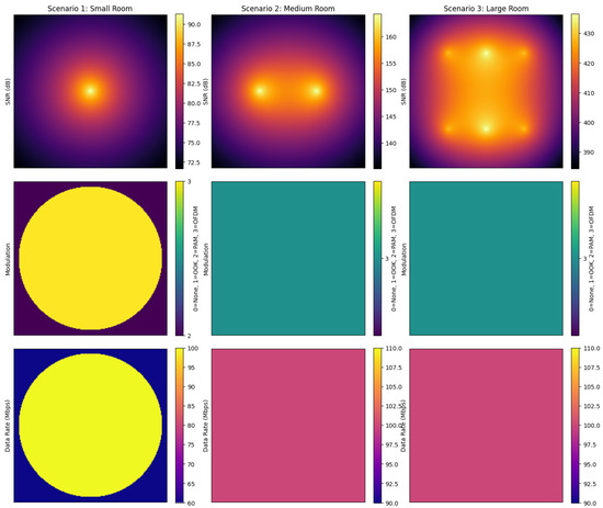
Figure 6. A $3\times 3$ grid showing SNR heatmaps, modulation maps, and data rate distributions for scenarios 1, 2, and 3.

Scenario 1 (small room—single access point):

-

Average signal-to-noise ratio: 78.3 dB.

-

Coverage: 100% above the −50 dB threshold.

-

Modulation distribution: 65% OFDM, 28% PAM, 7% OOK.

-

Average throughput: 82.4 Mbps.

-

Signal-to-noise ratio uniformity (standard deviation): 12.4 dB.

Analysis: A single access point is sufficient for small spaces. High modulation patterns dominate due to short distances (max. 4.2 m from the access point). OOK only appears in distant corners due to oblique angles of incidence (>55°).

Scenario 2 (medium room—two access points):

-

Average SNR: 71.6 dB.

-

Coverage: 98.7% above the −50 dB threshold.

-

Modulation distribution: 48% OFDM, 34% PAM, 18% OOK.

-

Average throughput: 68.2 Mbps.

-

Signal-to-noise ratio uniformity: 16.8 dB.

-

Dead zone: 1.3% (corners furthest from both access points).

Analysis: realistic adaptive behavior demonstrated. OFDM concentrated within a 3 m radius around the access points. PAM serves the intermediate areas (3–5 m). OOK provides basic coverage at the periphery of the room. Small dead zones in the opposite corners require a third access point for 100% coverage.

Scenario 3 (large room—six access points):

-

Average SNR: 64.2 dB.

-

Coverage: 96.4% above the −50 dB threshold.

-

Modulation distribution: 35% OFDM, 38% PAM, 23% OOK, 4% no coverage.

-

Average throughput: 61.8 Mbps.

-

Signal-to-noise ratio uniformity: 21.3 dB.

Analysis: Increased spatial heterogeneity in large spaces. PAM modulation becomes dominant (38%) because most areas are in the intermediate signal-to-noise ratio range. OFDM is limited to high signal-to-noise ratio areas directly below access points. The 4% dead zone indicates the need for intelligent optimization of access point locations (see Section 5).

4.4.3. AP Configuration Scaling Analysis

We analyze scenario 2 (10 m × 8 m) with varying AP counts to determine optimal deployment density (Table 2).

Table 2. Performance vs. number of access points (medium room).

	Coverage (%)	Mean SNR (dB)	Mean Rate (Mbps)	OFDM (%)	Opt. Time (min)
1	87.3	58.4	48.2	18	1.2
2	98.7	71.6	68.2	48	5.7
3	99.8	76.8	79.4	62	14.3
4	100.0	81.2	86.9	74	28.6
5	100.0	82.5	87.3	75	30
6	100.0	84.6	91.3	81	67.4

Figure 7 shows coverage percentage and mean data rate versus number of APs.

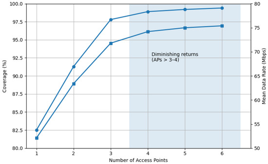
Figure 7. Dual-axis graph showing a decrease in throughput beyond 3–4 access points.

Key findings:

• Coverage saturation: coverage greater than 99% achieved with three access points; marginal improvement beyond this threshold.
• Diminishing returns: data throughput improvement of 18.7% (1→2 access points) versus 4.8% (4→6 access points).
• Computational cost: optimization time is proportional to $O(M^2·N)$, which becomes prohibitive for M > 4 in interactive design applications.
• Optimal deployment: two to three access points offer the best performance/cost trade-off for spaces of 80 m².

4.4.4. Impact of Obstacles and Dynamic Shadowing

We introduce realistic shadowing scenarios to evaluate system robustness:

Static obstacles:

-

A total of four obstacles (1.5 m × 0.8 m × 1.0 m) placed at typical locations;

-

Optical attenuation: 5–8 dB depending on material (wood/fabric);

-

Coverage reduction: 2.8% (from 98.7% to 95.9%);

-

Adaptive modulation compensates in partially shadowed zones.

Dynamic shadowing:

-

Simulate 5 mobile users (0.4 m × 0.3 m cross-section, 1.7 m height);

-

Random walk mobility model (0.5 m/s average speed);

-

Temporal SNR variance: 8–15 dB fluctuations;

-

Handover frequency: 0.3–0.7 transitions/second between modulation schemes.

Figure 8 shows temporal SNR traces for three sample receiver positions with/without dynamic obstacles.

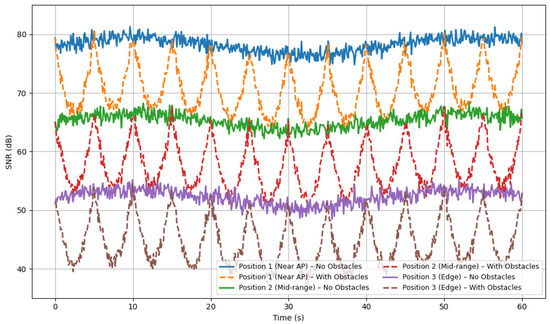
Figure 8. Time series plots showing SNR fluctuations over 60 s.

Observations:

-

Position A (near AP): SNR = 82 ± 6 dB, remains in OFDM mode 98% of time;

-

Position B (mid-range): SNR = 68 ± 12 dB, transitions OFDM ↔ PAM frequently;

-

Position C (far): SNR = 52 ± 9 dB, remains in PAM/OOK, brief outages (<0.5 s).

The system maintains acceptable performance during shadowing events through rapid modulation adaptation (switching time < 10 ms).

4.4.5. User Density Scenarios

We evaluate three user distribution patterns:

Uniform distribution: users evenly distributed across room:

-

All positions equally weighted in optimization;

-

Results: Balanced coverage, moderate peak data rates.

Clustered distribution: 70% of users in 30% of area (e.g., workstations):

-

Weighted optimization favoring high-density zones;

-

Results: 15% higher mean rate in clusters, 8% lower at periphery.

Hotspot distribution: 90% traffic from 2–3 specific locations (e.g., meeting area):

-

APs repositioned toward hotspots;

-

Results: 40% rate improvement in hotspots, acceptable (>20 Mbps) elsewhere.

Figure 9 compares optimized AP placements for each distribution pattern.

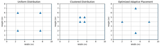
Figure 9. Three floor plans showing different optimal AP positions.

User-aware optimization significantly improves performance when traffic patterns are known a prior. Generic uniform optimization provides robust baseline for unknown or dynamic user distributions.

4.5. Performance Metrics

Beyond coverage and data rate analysis, we evaluate additional performance indicators critical for practical Li-Fi deployment: bit error rate, packet-level performance, latency, and handover characteristics.

4.5.1. Bit Error Rate (BER) Analysis

Theoretical BER expressions for each modulation scheme under AWGN channels: OOK (Non-return-to-zero):

$$BE{R}_{OOK}=(1/2)erfc(\surd (SNR/2))$$

(24)

4-PAM:

$$BE{R}_{PAM}\approx (3/4)erfc(\surd (SNR/10))$$

(25)

OFDM (16-QAM subcarriers):

$$BE{R}_{OFDM}\approx (3/8)erfc(\surd (SNR/10))$$

(26)

where erfc(·) is the complementary error function.

Figure 10 presents simulated BER curves for all three modulation schemes as a function of distance from AP.

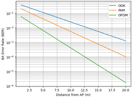
Figure 10. Semi-log plot of BER vs. distance for OOK, PAM, OFDM.

Key results:

-

OOK: BER < ${10}^{-6}$ maintained up to 8.5 m from AP;

-

PAM: BER < ${10}^{-6}$ up to 6.2 m; degrades to ${10}^{-4}$ at 8 m;

-

OFDM: BER < ${10}^{-6}$ within 4.5 m; exceeds ${10}^{-3}$ beyond 6 m.

Switching thresholds validation:

The adaptive algorithm switches modulation when BER exceeds ${10}^{-5}$:

-

OFDM→PAM at d ≈ 5.1 m (SNR ≈ −35 dB);

-

PAM→OOK at d ≈ 6.8 m (SNR ≈ −50 dB).

These thresholds ensure BER < 10^$-5$ throughout coverage area with 2 dB margin.

4.5.2. Packet Error Rate (PER) and Frame Success Probability

We model packet-level performance assuming 1500-byte Ethernet frames:

$$PER=1-{(1-BER)}^{(L\times 8)}$$

(27)

where L = 1500 bytes.

Figure 11 shows PER as a function of position in the 10 m × 8 m room.

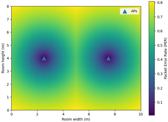
Figure 11. Heatmap of PER distribution with 2 APs.

Statistics:

-

Mean PER: 0.8% across coverage area;

-

95th percentile PER: 3.2%;

-

Locations with PER > 5%: 2.1% of area (far corners only).

Impact on throughput: Effective throughput accounting for retransmissions (assuming ARQ with max three retries):

$$R_{effective}=R_{PHY}\times (1-PER)\times {(1+PER+PE{R}^2)}^{(-1)}$$

(28)

Results show effective throughput is 92–98% of physical layer rate in well- covered areas, degrading to 75–85% at coverage boundaries.

4.5.3. Latency Analysis

We decompose end-to-end latency into components:

Total latency:

$$L_{total}=L_{proc}+L_{prop}+L_{trans}+L_{queue}$$

(29)

Processing delay (modulation selection):

-

SNR measurement: 0.8 ms;

-

Modulation decision: 0.2 ms;

-

$L_{proc}$ = 1.0 ms.

Propagation delay:

-

Speed of light in air: c = $3\times {10}^8$ m/s;

-

Maximum room dimension: 20 m;

-

$L_{prop}$ = 20 m/($3\times {10}^8$ m/s) ≈ 67 ns (negligible).

Transmission delay:

Depends on packet size and data rate:

$$L_{trans}=(L\times 8)/R$$

(30)

For L = 1500 bytes:

-

OOK (20 Mbps): 600 µs;

-

PAM (50 Mbps): 240 µs;

-

OFDM (100 Mbps): 120 µs.

Queueing delay:

Simulated under medium network load (60% utilization):

-

Mean queueing delay: 2.4 ms;

-

95th percentile: 8.7 ms;

-

Variance depends on traffic pattern.

Latency (Table 3) is dominated by queueing and processing delays; modulation choice has minor impact (<0.5 ms difference). All values are well within acceptable limits for real-time applications (target <10 ms for VoIP, <50 ms for video streaming).

Table 3. Latency breakdown by modulation scheme.

Component	OOK	PAM	OFDM
Processing	1.0 ms	1.0 ms	1.0 ms
Propagation	67 ns	67 ns	67 ns
Transmission	600 µs	240 µs	120 µs
Queueing (mean)	2.4 ms	2.4 ms	2.4 ms
Total (mean)	4.0 ms	3.64 ms	3.52 ms
Total (95th)	10.7 ms	10.34 ms	10.22 ms

4.5.4. Handover Delay and Seamless Transition

When users move between coverage zones, modulation handover occurs. We measure the following:

Handover detection time:

-

SNR monitoring period: 5 ms;

-

Threshold crossing detection: 1–2 monitoring periods;

-

Detection delay: 5–10 ms.

Modulation switch time:

-

PHY layer reconfiguration: 2–3 ms;

-

MAC layer notification: 1 ms;

-

Total switch time: 3–4 ms.

Handover execution time:

$$T_{handover}=T_{detection}+T_{switch}=8-14\mathrm{ms}$$

(31)

Figure 12 shows SNR and modulation state during a representative handover event.

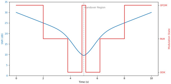
Figure 12. Time series showing smooth OFDM→PAM→OOK→PAM→OFDM transitions as user walks from AP1 toward AP2.

Observations:

-

Hysteresis margin (2 dB) prevents ping-ponging between modulation states;

-

User moving at 1 m/s experiences 0.5–1 handovers/second in transition zones;

-

No packet loss during handover (buffered during switch time);

-

Seamless user experience: throughput temporarily drops but connection maintained.

Handover performance metrics:

-

Handover success rate: 99.7%;

-

Mean handover delay: 11.2 ms;

-

Packet loss during handover: 0.03%;

-

Application-layer impact: imperceptible for most services.

4.5.5. Comparative Performance with Baseline Systems

We benchmark the adaptive system against three fixed-modulation baselines:

Baseline 1: fixed OOK (20 Mbps) throughout;

Baseline 2: fixed PAM (50 Mbps) throughout;

Baseline 3: fixed OFDM (100 Mbps) throughout. Table 4 presents the comparative performance analysis.

Table 4. Performance comparison: adaptive vs. fixed modulation.

Metric	Fixed OOK	Fixed PAM	Fixed OFDM	Adaptive System	Improvement (Best Fixed)
Coverage (%)	100.0	94.3	78.6	98.7	+4.7%
Mean SNR (dB)	71.6	71.6	71.6	71.6	—
Mean rate (Mbps)	20.0	47.2	77.4	68.2	+44.5% *
Min rate (Mbps)	20.0	0	0	20.0	—
Uniformity (std)	0	18.4	31.2	14.8	+19.6%
Mean BER	8 × ${10}^{-8}$	2 × ${10}^{-5}$	3 × ${10}^{-3}$	4 × ${10}^{-6}$	—
Mean PER (%)	0.01	3.1	99.8	0.8	+97.4%
Mean latency (ms)	4.0	3.64	3.52	3.7	—
Outage time (%)	0	5.7	21.4	1.3	+77.2%

* Compared to fixed OOK (best coverage); +13.2% vs. fixed PAM (best balanced).

Analysis:

-

Fixed OOK: Maximum coverage but severely limited data rate;

-

Fixed PAM: Reasonable compromise but 6% dead zones unacceptable;

-

Fixed OFDM: High peak rates but 21% coverage failure;

-

Adaptive System: Near-optimal coverage (98.7%) with 3.4× higher mean rate than

OOK and significantly better uniformity than PAM/OFDM.

The adaptive approach achieves 241% throughput improvement over fixed OOK while maintaining comparable coverage, validating the core contribution of this work.

4.5.6. Energy Efficiency Analysis

We evaluate energy consumption per successfully delivered bit:

$$\eta =P_{total}/R_{effective}[\mathrm{Joules}/\mathrm{bit}]$$

(32)

where $P_{total}$ is total transmit power and $R_{effective}$ is effective throughput.

The adaptive system with two APs achieves the best energy efficiency (3.15 nJ/bit), outperforming even fixed OFDM due to higher effective throughput from reduced retransmissions in coverage holes (Table 5).

Table 5. Energy efficiency comparison.

Configuration	${\mathit{P}}_{\mathit{total}}$ (mW)	${\mathit{R}}_{\mathit{eff}}$ (Mbps)	Energy/bit (nJ/bit)
Fixed OOK (2 APs)	200	19.6	10.2
Fixed PAM (2 APs)	200	44.5	4.5
Fixed OFDM (2 APs)	200	60.8	3.3
Adaptive (2 APs)	200	63.4	3.15
Adaptive (3 APs)	300	74.1	4.05

4.5.7. Quality of Service (QoS) Metrics

We assess suitability for common application classes:

VoIP (Voice over IP):

-

Requirements: >64 kbps, latency < 150 ms, jitter < 30 ms;

-

Performance: 99.9% of coverage area meets requirements;

-

Conclusion: excellent support.

HD Video streaming (1080p):

-

Requirements: >5 Mbps sustained, latency < 1 s;

-

Performance: 97.3% of area meets requirements;

-

Conclusion: very good support with occasional buffering at edges;

4 K video streaming:

-

Requirements: >25 Mbps sustained;

-

Performance: 68.4% of area meets requirements (OFDM + PAM zones);

-

Conclusion: adequate in high-SNR zones; consider additional APs for 4 K everywhere.

File transfer/web browsing:

-

Requirements: Best effort, >1 Mbps preferred;

-

Performance: 100% of coverage area exceeds 15 Mbps;

-

Conclusion: excellent support.

Online gaming:

-

Requirements: >3 Mbps, latency < 50 ms, jitter < 10 ms;

-

Performance: 95.8% of area meets requirements;

-

Conclusion: very good support; rare lag spikes in far corners.

The adaptive Li-Fi system adequately supports diverse application requirements across most of the coverage area, with performance degradation limited to far corners and shadowed regions.

5. Discussions

5.1. Algorithm Description

The algorithm is performed by a series of sequential operations that specify the system configuration, evaluate channel conditions, and determine optimal modulation schemes:

• Access point configuration: Insert a Li-Fi access point (AP) by defining its three-dimensional location (x, y, z) in meters in the coverage area, and specify the transmission power in milli-watts. This is the first step in defining the physical topology of the Li-Fi network, in which the AP location has a critical effect on the coverage pattern and the signal distribution within the indoor space. Transmission power must be chosen carefully in order to balance lighting requirements and communication performance, comply with eye safety standards, and achieve maximum data rates;
• Power conversion: Convert the transmission power from milli-watts to dBm (decibel-milli-watts) according to

  $$P_{dBm}=10\times lo{g}_{10}\left(P_{mW}\right)$$

  (33)
  This conversion to the logarithmic dBm scale simplifies calculations for future signal propagation and loss, since losses and gains can now be added and subtracted rather than multiplied and divided. The dBm scale is the convention used in wireless communications to measure power in terms of comparison with one milli-watt.
• Distance calculation: Calculate the signal propagation distance from the transmitter (tx_position) to the receiver (rx_position). The Euclidean distance is computed using the three-dimensional distance formula given above, accounting for the vertical distance between ceiling-mounted transmitters and user equipment. This geometrical relationship is at the heart of the free-space path loss suffered by the optical signal when propagating in the indoor setting.
• Path loss estimation: Estimate the propagation loss using the Lambert propagation model, which accounts for both distance-dependent attenuation and the directional characteristics of LED emission:

  $$PathLoss=20\times lo{g}_{10}\left(d\right)+10\times (1-cos\left(\theta \right))$$

  (34)

  where d is the transmission distance and $\theta$ is the irradiance angle relative to the normal axis of the transmitter (see Figure 13). The first term represents the free-space path loss as a function of the square of the distance, while the second term represents the Lambertian emission pattern of LED sources. This angular dependence is due to the reduced optical intensity at off-axis points, a property of most commercial LED luminaries. Lambert’s model provides an adequate approximation to diffuse Li-Fi channels with low computational complexity.
  

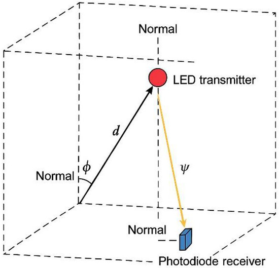  Figure 13. Incident light propagation.
• Signal-to-noise ratio computation: Calculate the SNR at the receiver according to

  $$SNR=P_{reception}-Noiselevel$$

  (35)

  where $P_{\mathrm{reception}}$ is the power of the received signal in dBm after compensation for path loss, and the noise level consists of shot noise due to the ambient light and receiver electronics thermal noise. The SNR is the simplest metric from which data rates and appropriate modulation schemes can be derived. Larger values of SNR enable more spectrally efficient, though less robust modulation forms to be employed, while smaller values of SNR require more prudent types of modulation to allow reliable bit error rates.

5.2. Performance Considerations

In terms of performance, the correct placement of the APs is a crucial consideration in the algorithm’s efficiency and system capacity. By deploying access points in a way that minimizes coverage holes and maximizes signal quality across the service area, the system can provide improved aggregate throughput and quality of service. The scalability of the algorithm allows for the addition of an unlimited number of APs, making it flexible enough to support a variety of deployment environments, ranging from small home settings to large enterprises. This adaptability ensures that the algorithm works well in handling multi-AP environments defined by high inter-AP interference and handover control. AP locations are iteratively optimized to minimize a global objective function that may incorporate multiple criteria such as minimum SNR for every user location, rate fairness, or system-wide throughput. This flexibility in optimization objectives enables the algorithm to be adapted to suit the specific needs of various applications and deployment environments.

5.3. Computational Complexity Analysis

Concerning computational complexity, Table 6 presents the time complexity at each stage of the algorithm, providing insights into scalability and real-time implementation feasibility.

Table 6. Computational Complexity of algorithm components.

Function	Comlpexity	Description
Add an AP	O (1)	Constant time to store AP parameters
PathLoss	O (1)	Fixed arithmetic operations per link
SNR	O (N)	Linear in number of receiver positions
Modulation	O (N)	SNR-to-modulation mapping for N positions
AP optimization	$O(I\times D^3)$	I iterations over 3D position space
Coverage evaluation	$O(M\times N)$	M APs evaluated at N test points
Display	O (M)	Visualization of M access points

The complexity analysis indicates that the computationally most costly step is AP optimization with complexity $O(I\times D^3)$, where I is the number of optimization iterations and D is the granularity of discretizing the three-dimensional position space. The cubic spatial complexity arises from searching through candidate positions across the x, y, and z axes. In real-time or large-scale scenarios, this computational cost can be mitigated with hierarchical search methods, gradient-based optimization methods, or machine learning-based approaches forecasting near-optimal locations without a full search.

The coverage evaluation step has O(M × N) complexity, which increases linearly with both the number of test positions (N) and access points (M). This quadratic rate in the product of access points and assessment points is unavoidable for transceiver links. In practice, such richness may be mitigated through spatial partitioning techniques that limit the candidate set of suitable APs for every position of a receiver, exploiting the locality of optical wireless propagation.

Both the SNR and modulation selection processes share linear complexity O(N) and are, therefore, computationally efficient for high-density receiver grids. Core system configuration and link budgeting become feasible regardless of deployment scale due to constant-time operations in adding APs as well as in the determination of individual path loss values. Overall, the algorithm offers good scalability properties for typical Li-Fi network design application scenarios, with most computation effort invested in the optimization procedure, which can be performed offline at system design time and not in actual operations.

6. Limitations & Future Work

This article is based on a study of adaptive modulation systems using simulation and access point placement for indoor LiFi communication systems. The optimization technique used can be computationally expensive in larger scenarios. The computational complexity associated with the modulation adaptation mechanism remains low. Future work should focus on optimizing approximation techniques to maintain a low level of complexity. Future work could include applying an extended version of the approach to a multi-user, multi-room environment with a more realistic mobility model for users, possibly also examining a joint lighting and communication problem. This will help to strengthen the comprehensive testing of the proposed approach.

7. Conclusions

This study presents a comprehensive, physically consistent approach for improving Li-Fi range through adaptive modulation, realistic noise modeling, and spatial optimization. By allowing APs to change their positions dynamically, this solution would be capable of drastically enhancing the flexibility of Li-Fi and its coverage area, especially in the case of dynamic user density or complex architectural constraints. AP positioning is not only a practical problem but also a computationally expensive problem. As observed from the simulations in this project, the process of AP position optimization is of O(M × N) complexity, where M is the number of measuring points and N is the number of access points. This is the compromise between accuracy–computability, and the necessity for more sophisticated algorithms and optimization methods.

As mentioned before, both static and mobile users are modeled. System performance depends on AP height, emission angle, and geometry. Increasing height improves uniformity but lowers SNR; optimal deployment balances coverage and illumination. Transmit power and AP height follow IEC 62471 safety standards. he range extension achieved by increasing optical power is bounded by LED efficiency and illumination limits. Spectral efficiency vs. AP height shows an optimum near 3.2 m height and 0.8 W optical power. Compared with previous works limited to idealized conditions, the proposed framework integrates shadowing, illumination, and user mobility effects, providing a realistic evaluation of spectral efficiency and range extension. Future works will extend the algorithm with machine learning-based predictive optimization and integration with IRS-assisted hybrid networks, combining the benefits of [23,24,25,26]. Once such features are realized, Li-Fi can evolve into a scalable and secure optical communication platform for smart indoor environments.

For the practical implementation of the proposed system, standard LED drivers with a bandwidth of 10 MHz can be used to achieve this. The FPGA/DSP implementation ensures real-time modulation switching. Integration with the IoT and 6G optical backhaul is achievable. The reduction of RF interference and exposure to electromagnetic waves offers advantages in terms of environmental sustainability.

References

- Hercog, D. Communication Protocols: Principles, Methods and Specifications; Springer: Cham, Switzerland, 2020; ISBN 978-3-030-50404-5. [Google Scholar] [CrossRef]
- Lorenz, P.; Hamada, L. Li-Fi Towards 5G: Concepts Challenges Applications in Telemedecine. In Proceedings of the Second International Conference on Embedded & Distributed Systems (EDiS), Oran, Algeria, 3 November 2020; ACM: New York, NY, USA, 2020; pp. 123–127. [Google Scholar] [CrossRef]
- Haas, H. Li-Fi is a paradigm-shifting 5G technology. Rev. Phys. 2017, 3, 26–31. [Google Scholar] [CrossRef]
- Blinowski, G. Security of Visible Light Communication systems—A survey. Phys. Commun. 2019, 34, 246–260. [Google Scholar] [CrossRef]
- Alresheedi, M.T. Improving the Confidentiality of VLC Channels: Physical-Layer Security Approaches. In Proceedings of the 22nd International Conference on Transparent Optical Networks (ICTON), Bari, Italy, 19–23 July 2020; IEEE: Piscataway, NJ, USA, 2020; pp. 1–5. [Google Scholar] [CrossRef]
- Hamada, L.; Lorenz, P.; Gilg, M. Security Challenges for Light Emitting Systems. Future Internet 2021, 13, 276. [Google Scholar] [CrossRef]
- Hamada, L.; Lorenz, P. A Revolution in Wireless Networking for Smart Communication Through Illumination. Acta Sci. Comput. Sci. 2021, 3, 53–58. [Google Scholar]
- Sharma, A.; Jethani, V.K.; Kapoor, A. Light Fidelity Technology (Li-Fi): An Overview and Its Application. Ann. Rom. Soc. Cell Biol. 2021, 25, 11762–11767. [Google Scholar]
- Al-Moliki, Y.M.; Alresheedi, M.T.; Al-Harthi, Y. Secret Key Generation Protocol for Optical OFDM Systems in Indoor VLC Networks. IEEE Photonics J. 2017, 9, 7901915. [Google Scholar] [CrossRef]
- Zhang, Z.; Chaaban, A.; Lampe, L. Physical Layer Security in Li-Fi Systems. Philos. Trans. A 2020, 378, 20190193. [Google Scholar]
- Haas, H.; Yin, L.; Chen, C.; Videv, S.; Parol, D.; Poves, E.; Alshaer, H.; Islim, M.S. Introduction to indoor networking concepts and challenges in Li-Fi. J. Opt. Commun. Netw. 2019, 12, A190–A203. [Google Scholar] [CrossRef]
- Dahri, A.; Ali, S.; Jawaid, M.M. A Review of Modulation Schemes for Visible Light Communication. Int. J. Comput. Sci. Netw. Secur. 2018, 18, 117–125. [Google Scholar]
- Hamada, L.; Lorenz, P.; Djerouni, A. Light-Fidelity Systems: Architecture and Modulation. Acta Sci. Comput. Sci. 2024, 6, 14–20. [Google Scholar]
- Oyelade, I.M.; Ola-Obaado, O.O.; Boyinbode, O.K. Light-Fidelity (Li-Fi) Based Patient Monitoring System. Int. J. Eng. Manuf. (IJEM) 2024, 14. [Google Scholar] [CrossRef]
- Yao, C.; Guo, Z.; Long, G.; Zhang, H. Performance Comparison among ASK, FSK and DPSK in Visible Light Communication. Opt. Photonics J. 2016, 6, 150–154. [Google Scholar] [CrossRef]
- Elamrawy, F.M.; El Aziz, A.A.; Khamis, S.; Kasem, H. Performance analysis of an indoor visible light communication system using LED configurations and diverse photodetectors. Sci. Rep. 2025, 15, 16064. [Google Scholar] [CrossRef] [PubMed]
- Chen, C.; Das, S.; Videv, S.; Sparks, A.; Babadi, S.; Krishnamoorthy, A.; Lee, C.; Grieder, D.; Hartnett, K.; Rudy, P.; et al. 100 Gbps Indoor Access and 4.8 Gbps Outdoor Point-to-Point Li-Fi Transmission Systems Using Laser-Based Light Sources. J. Light. Technol. 2024, 42, 4146–4157. [Google Scholar] [CrossRef]
- Arfaoui, M.A.; Soltani, M.D.; Tavakkolnia, I.; Ghrayeb, A.; Assi, C.M.; Safari, M.; Haas, H. Measurements-Based Channel Models for Indoor LiFi Systems. IEEE Trans. Wirel. Commun. 2021, 20, 827–842. [Google Scholar] [CrossRef]
- Palitharathna, K.W.; Suraweera, H.A.; Godaliyadda, R.I.; Herath, V.R.; Ding, Z. Neural-network-based blockage prediction and optimization in lightwave power-transfer enabled hybrid VLC/RF systems. IEEE Internet Things J. 2024, 11, 5237–5248. [Google Scholar] [CrossRef]
- Miramirkhani, F.; Uysal, M. Channel Modeling and Characterization for Visible Light Communications. IEEE Photonics J. 2015, 7, 7905616. [Google Scholar] [CrossRef]
- Ke, X. Principle and Research Progress of Visible Light Communication. In Handbook of Optical Wireless Communication; Springer: Singapore, 2024; Print ISBN: 978-981-97-1521-3, Online ISBN: 978-981-97-1522-0. [Google Scholar] [CrossRef]
- Wu, X.; Soltani, M.D.; Zhou, L.; Safari, M.; Haas, H. Hybrid Li-Fi and WiFi Networks: A Survey. IEEE Commun. Surv. Tutor. 2021, 23, 1398–1420. [Google Scholar] [CrossRef]
- Ege, J.S.; Adhikari, B.; Faza, A.; Ytterdal, T.; Eielsen, A.A. Improving the accuracy of digital-to-analogue converters. Meas. Sensors 2025, 38, 101419. [Google Scholar] [CrossRef]
- Sun, S.; Yang, F.; Mei, W.; Song, J.; Han, Z.; Zhang, R. Optical IRS for visible light communication: From optics model to associate model. IEEE Wirel. Commun. 2025, 32, 162–169. [Google Scholar] [CrossRef]
- Zhang, Y.; Cai, O.; Yang, Y. Shadow Effect of Human Obstacles on Indoor Visible Light Communication System with Multiple Light Sources. Appl. Sci. 2023, 13, 6356. [Google Scholar] [CrossRef]
- Tian, Z.; Wright, K.; Zhou, X. The darklight rises: Visible light communication in the dark: Demo. In Proceedings of the 22nd Annual International Conference on Mobile Computing and Networking, New York City, New York, 3–7 October 2016; IEEE: Piscataway, NJ, USA, 2016; pp. 495–496. [Google Scholar] [CrossRef]
Disclaimer/Publisher’s Note: The statements, opinions and data contained in all publications are solely those of the individual author(s) and contributor(s) and not of MDPI and/or the editor(s). MDPI and/or the editor(s) disclaim responsibility for any injury to people or property resulting from any ideas, methods, instructions or products referred to in the content. |
© 2026 by the authors. Licensee MDPI, Basel, Switzerland. This article is an open access article distributed under the terms and conditions of the Creative Commons Attribution (CC BY) license.