Predictive Modelling of Erosion Behaviour in Polymeric and Composite Materials Using Machine Learning

Abstract

Accurate prediction of erosion rates in polymeric and composite materials is essential for their effective design and maintenance in diverse industrial environments. This study presents a predictive modelling framework developed using the JMP Pro machine learning integrated system to estimate erosion rates of polymers and polymer composites. For better model generalisation under various conditions, a curated dataset was compiled from peer-reviewed literature, standardised, and subjected to outliers and multivariate exploratory data analysis to identify dominant variables. The model utilises key input parameters, including impact angle, impact velocity, sand content, particle size, material type, and fluid medium, to predict the erosion rate as the target output variable. Six machine learning algorithms were evaluated through a systematic model comparison process, and two were selected. Model performance was assessed using robust error metrics, and the interpretability of erosion behaviour was validated through prediction profilers and variable importance analyses. Artificial Neural Network (ANN) and Extreme Gradient Boosting (XGBoost) demonstrated the best training and validation performance based on the evaluation metrics. While both models yielded high training performance, the ANN model demonstrated superior predictive accuracy and generalisation capability across a broad range of conditions. Beyond prediction, the model outputs also showed a meaningful representation of the influence of input variables on erosion rates.

1. Introduction

Polymers and their composites have witnessed a growing utilisation in a wide array of engineering applications, particularly within the aerospace, marine, offshore, mining, and energy sectors. This growth is largely driven by their favourable properties, including a high strength-to-weight ratio, excellent corrosion resistance, low manufacturing cost, and flexibility in tailoring properties for specific functional requirements [1]. These attributes make them promising substitutes for traditional metallic components, particularly valuable in environments where weight reduction and durability are critical [2].

Despite these advantages, polymeric materials are still susceptible to surface degradation when exposed to erosive environments. The repeated impingement of solid particles and the associated micro-mechanical interactions can lead to progressive material loss, surface damage, and a reduction in mechanical performance over time [3,4]. This degradation is especially critical in dynamic flow systems, where erosion can compromise structural reliability and increase maintenance costs. As a result, erosion resistance has become a key factor in material selection, particularly for applications involving erosive flows or particulate-laden fluids. A robust understanding of erosion behaviour is now essential for service-life prediction and material selection in such aggressive environments.

Erosive wear in polymers and polymer composites is a complex phenomenon governed by a combination of factors, including the properties of the impacting particles, flow velocity, impingement angle, environmental conditions, and the material’s physical and structural characteristics [5]. In composites, the addition of reinforcements further influences erosion behaviour by altering material response under dynamic loading. These variables collectively determine the severity and progression of material loss, making erosive wear a critical consideration in the performance and durability of polymer-based components across various industrial applications.

Traditional erosion modelling has primarily relied on empirical correlations, which are often derived from specific laboratory test configurations and narrowly defined material systems. While these models provide initial insights, their applicability is usually confined to the range of input conditions for which they were calibrated [6,7,8,9,10].

Machine learning (ML) has emerged as a powerful alternative approach for predictive modelling, particularly in contexts where traditional empirical correlations fail to capture the full complexity of system behaviour. ML is a subfield of artificial intelligence that enables computers to learn from data and improve their performance on tasks without being explicitly programmed for them. It focuses on the development of algorithms that can identify patterns in data and make predictions or decisions based on those patterns, often generalising to new, unseen data [11].

In erosion studies, the degradation of materials is governed by nonlinear, multivariable interactions between process parameters, such as impact velocity, impingement angle, particle concentration, and material properties. Conventional models, often limited by assumptions of specific materials and boundary conditions, are unable to generalise across diverse datasets or accommodate such complex interdependencies [11].

In contrast, ML algorithms can handle large, diverse datasets and capture complex, nonlinear relationships between multiple variables, making them well-suited for identifying hidden patterns and data-driven prediction in challenging scenarios without requiring predefined functional forms. Modern ML frameworks also support model interpretability through tools like feature importance metrics and prediction profilers, enabling researchers to identify the dominant factors influencing erosion and guide design improvements [12].

JMP Pro (version 18, SAS Institute Inc., Cary, NC, USA) statistical and machine learning software was selected as the modelling platform in this study due to its strong emphasis on advanced predictive modelling and automated model selection and validation, making it a preferred tool for data-driven studies [13]. Its no-code interface supports efficient data exploration, preprocessing, and model building, enabling users to perform complex analyses without extensive programming expertise. The software is designed with a clean and intuitive layout that minimises cognitive overload; each output is accompanied by a contextual menu, simplifying workflow navigation. JMP Pro is also highly visual, and almost every step in the analysis is graphical and interactive. When users engage with a graphical object, related outputs update dynamically, supporting real-time pattern recognition and knowledge discovery. Additionally, the JMP Scripting Language (JSL) enables advanced customisation and integration with external platforms such as SAS, R, Python, and MATLAB, offering flexibility for extended analytical tasks [14].

ML has shown significant potential in modelling complex tribological behaviour, and several studies have successfully applied these techniques to metals and ceramics under various conditions. However, their use in predicting erosion in polymers and composites remains insufficiently developed [15,16,17,18,19,20,21].

Many existing ML-based erosion models are restricted in scope, focusing on a narrow selection of polymeric materials and test parameters, thereby limiting their generalisability across the diverse erosion scenarios encountered in practice [18,20,21].

Another key shortcoming is that most predictive models remain at a conceptual stage, with insufficient emphasis on interpretability or validation that connect predictions with underlying physical mechanisms [18,19,20,21].

Furthermore, the practical applicability of predictive models remains limited. Most Existing models are rarely translated into deployable formats that can be accessed or used outside their development environments.

To advance the field and address these gaps, this study aims to develop a generalised machine learning-based predictive erosion model that covers a broader scope of polymeric materials and test conditions, provides physical interpretations of the prediction performance and variable effects, and demonstrates practical deployment capability for integration into external systems. The approach leverages the tools of JMP Pro. The specific objectives include:

• Compile a wide range of erosion datasets and materials from peer-reviewed literature, ensuring consistency through unit normalisation, dimensional analysis, and removal of outliers.
• Perform exploratory analysis to identify statistically significant variables using correlation studies, interaction effects, and multicollinearity assessment.
• Train and validate multiple ML algorithms to determine the best-performing model based on error metrics and physical plausibility.
• Perform model interpretation using prediction profilers and feature importance rankings to evaluate the influence of input variables on the predicted erosion rate.
• Deploy the trained models into usable Python scripts or other tools, facilitating application in external platforms or embedded systems.

2. Methodology

2.1. Data Collection and Preprocessing

2.1.1. Data Collection Criteria

The success of any machine learning predictive modelling largely depends on the quality and consistency of the data used to train it [22]. In this work, a dataset was carefully compiled from previously published studies focused on the erosion behaviour of polymers and polymer composites. This approach was chosen to ensure a broad and diverse representation of test conditions, material systems, and erosion mechanisms [22].

These studies were selected based on the following key criteria: (1) the use of polymers or polymer composites as the target material, (2) the availability of quantitative erosion rate measurements under liquid–sand or air–sand erosion conditions, and (3) the clear documentation of the testing procedures and the main variables affecting erosion, including impact velocity, impingement angle, sand content, material properties, and test duration. Following the application of these criteria, eleven peer-reviewed publications were selected to form the basis of the compiled dataset, ensuring methodological consistency and relevance to the scope of this study [9,16,23,24,25,26,27,28,29,30,31].

To build the dataset, each selected paper was thoroughly reviewed and analysed. Relevant information was extracted manually from tables and text. In several cases, numerical data were not directly reported in tables but were instead presented as plotted graphs within the published figures. To accurately recover these values, a reliable graph digitisation method was employed using PlotDigitizer, an open-source, browser-based tool widely used in research for this purpose [32]. The digitisation process began by uploading the selected image of the plot into the software interface. To ensure the accuracy of data extraction, both the horizontal (x-axis) and vertical (y-axis) scales were first calibrated using the reference tick marks or axis labels visible on the original plot. Once the scale was set, data points corresponding to the erosion rate or the relevant test variable were manually traced, and the tool provided the corresponding reading.

Special attention was given to ensure that the erosion test data were based on comparable testing methods, particularly jet-type impingement systems, which are widely employed in erosion research for their ability to deliver controlled and repeatable test conditions. To further ensure consistency across the compiled dataset, all extracted erosion rate values and related input parameters were carefully reviewed and, where necessary, converted into standardised units. The following input features were recorded for each test case:

• Material (polymers and polymer composites).
• Fluid type (water and air).
• Impact velocity (m/s).
• Impact angle (deg.).
• Sand content (concentration) (wt.%).
• Surface material hardness (Vickers hardness, HV).
• Erodent particle size (μm).
• Test duration (h).
• Measured erosion rate (mg/(mm²·year)).

These seven factors (material type, material hardness, particle size, impact angle, velocity, sand concentration, and fluid type) were chosen because they are universally recognised in erosion science as the primary drivers of erosion rate. Material hardness determines a polymer’s resistance to surface damage and energy dissipation during impact. Impact velocity and angle, together with particle size and sand concentration, govern the energy, frequency, and orientation of erosive interactions, directly affecting the severity and mode of material loss. Fluid type influences both the transport of abrasive particles and the impact regime. These parameters are not only the most influential according to the tribological literature but are also those that are most consistently and comprehensively reported across the available experimental studies in the literature. Their inclusion ensures that the resulting data-driven models are both physically meaningful and broadly applicable within a wide range of erosion conditions.

Each data point in the final dataset represents a unique erosion test, along with its corresponding conditions and results. In total, 186 test cases were compiled and organised into a structured dataset, which was then imported into the JMP Pro 18 system for further analysis.

By utilising data from multiple studies, this dataset reflects a diverse range of erosion conditions, which is essential for training a predictive model that performs well across different materials and environments. This approach also increases the reliability and practical value of the model when applied in real-world applications, such as material selection or erosion-resistant design.

2.1.2. Outlier Analysis

Identifying outliers is a crucial step in predictive modelling, as anomalous observations can disproportionately influence model fitting, introduce bias, and impair generalisation capability. Therefore, outlier detection was performed prior to model development. This step is essential in data pre-processing, particularly for machine learning applications. The detection process involved calculating the Jackknife Mahalanobis distance for each observation. This distance is plotted in Figure 1 (top) and represents a multivariate statistical measure that indicates how far each data point deviates from the average correlation structure of the remaining dataset, with this average recalculated each time by leaving out the point being evaluated [33,34]. This leave-one-out approach ensures that extreme outliers do not bias the multivariate mean of the distribution, thereby providing a more accurate detection of anomalies. If an extreme outlier is included in the calculation of the mean, it can pull the mean toward itself, masking its own deviation. The jackknife method avoids this by excluding the point prior to calculating the mean.

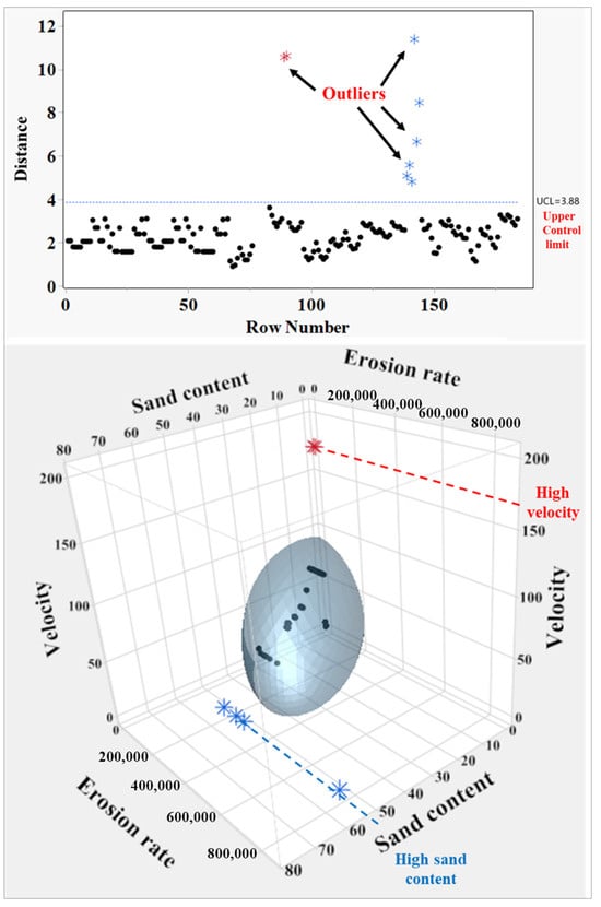
Figure 1. Identification of multivariate data outliers: (top): distance plot with UCL; (bottom): 3D scatter plot highlighting outliers. Black dots represent data points; red asterisks indicate high velocity outliers, and blue asterisks indicate high sand content outliers.

To separate genuine outliers from normal data variation, an Upper Control Limit (UCL), a statistical threshold, was established and is represented by the horizontal line in Figure 1. This limit is calculated using principles of multivariate quality control to define the 95% confidence boundary. Any observation whose Jackknife distance exceeds this UCL is deemed statistically inconsistent with the rest of the dataset, having less than a 5% probability of belonging to the same population structure. Observations exceeding this threshold were therefore treated as multivariate outliers and removed from the modelling dataset.

To better visualise the source of these deviations, the lower panel presents a three-dimensional scatter plot visualising the relationship among three key variables: erosion rate, sand content, and velocity. The majority of data points cluster within an ellipsoid, representing the typical distribution of the data. Outliers identified in the top panel are also shown here outside this region, with red asterisks indicating points with unusually high velocity and blue asterisks indicating points with high sand content, corresponding to extreme test conditions. Therefore, these outliers were excluded from the modelling dataset.

After removing outliers, the final dataset incorporated a diverse range of materials and experimental parameters. Table 1 provides a summary of the input variables, including their descriptions, units, and observed ranges within the dataset.

Table 1. Summary of input variables, descriptions, units, and observed ranges in the curated dataset following outlier exclusion.

Variable Name	Description	Unit	Range in Dataset
Surface material	Type of polymer or composite	-	CFRP, GFRP, HDPE, EP, PP, PEEK, GF-PEEK, CF-PEEK, GF-PEKK, CF-PEKK
Fluid type	Type of fluid medium	-	Air, Water
Hardness	Material hardness	Vickers hardness, HV	2.85–112.00
Sand content	Silica sand concentration in the medium	wt.%	0.00–38.37
Particle size	Sand particle size	μm	0–300
Impact angle	Impingement angle between erodent and material surface	degrees	5–90
Velocity	Jet or particle impact velocity	m/s	2.00–66.00
Erosion rate	Measured erosion rate	mg/(mm2·year)	0.09–135,442.19

2.1.3. Exploratory Data Analysis

To assess the statistical dependencies and interactions among the input variables and their influence on the target output (erosion rate) prior to predictive modelling, a correlation matrix coupled with a scatterplot matrix was generated. As shown in Figure 2, the upper part displays the Pearson correlation coefficients between each pair of variables. This approach provides a robust means of visualising and quantifying dependencies between each input variable and the erosion rate, as well as between each pair of variables. The coefficients range from −1 to +1, where values closer to +1 indicate a strong positive linear relationship, values near −1 indicate a strong negative linear relationship, and values around 0 suggest a weak or no linear association [12]. The erosion rate shows a positive correlation with sand content and velocity, while other variables have a relatively less significant influence. Notably, most input variables exhibit weak or negligible correlation with each other, indicating minimal multicollinearity, which is favourable for successful predictive modelling. The scatterplot matrix in the lower part visualises the pairwise relationships between variables and identifies any distribution that may not be evident from the correlation coefficients alone. Each off-diagonal cell contains a scatterplot for a specific variable pair, revealing trends, patterns, or clustering within the data. The ellipse in each scatterplot represents the bivariate normal density contour for the corresponding variable pair. Under the assumption of a bivariate normal distribution, approximately 95% of the data points are expected to lie within the ellipse. A narrow, diagonally oriented ellipse indicates a strong linear correlation, whereas a wider, more circular shape suggests a weak correlation between the two variables [12]. Sand content and velocity plots show elongated ellipses trending positively with erosion rate, consistent with their correlations. Meanwhile, plots involving impact angle or particle size display more circular or diffuse shapes, highlighting the lack of strong linear trends. The diagonal cells display histograms, providing insight into the distribution of each individual variable. The low coefficient value between impact angle and erosion rate arises from the nonlinear nature of their relationship; erosion typically peaks at intermediate angles, a pattern not captured by simple linear metrics. Similarly, the unexpected positive coefficient value between hardness and erosion is likely due to the varied material type in the dataset. Since different materials (polymers and composites) respond differently to erosive conditions, aggregating them without accounting for material classification can mask the expected inverse relationship between hardness and erosion resistance.

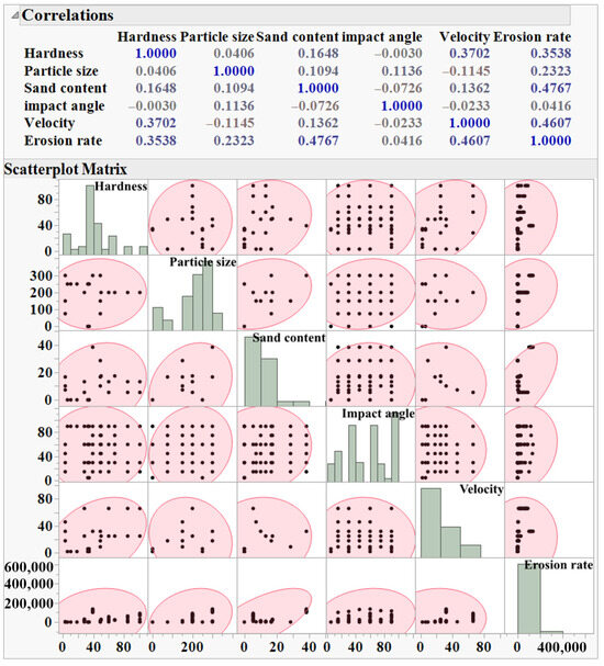
Figure 2. Correlation and scatterplot matrices illustrating relationships between input variables and erosion rate. Blue font in the correlation matrix highlights values closer to 1.

To complement the previous analysis, Figure 3 provides a heatmap view of the correlation structure. It offers a clear visual summary of linear relationships and supports earlier observations regarding the complexity and variability in how different factors influence the response.

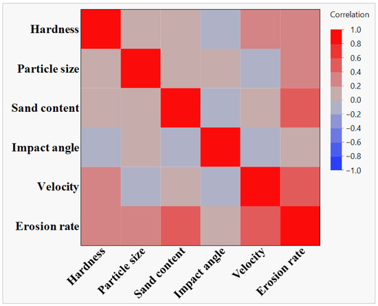
Figure 3. Heatmap of correlation coefficients, visually summarising the strength and direction of linear relationships among variables.

2.2. Machine Learning Model Comparison and Selection

Selecting the most suitable predictive algorithm is a crucial step in developing effective machine learning models, particularly for complex engineering systems. The erosion behaviour of polymers and their composites is governed by nonlinear, multidimensional interactions of material characteristics and operational parameters. These challenging dependencies call for a robust and flexible data-driven modelling framework that can capture higher-order interactions and generalise effectively across diverse conditions. There is no single method that universally outperforms others across all datasets or problem types. A practical approach involves applying multiple techniques and then selecting the one that demonstrates superior performance based on a comparative evaluation of model fit and predictive accuracy [14].

To address this objective, a comprehensive model screening process was conducted using the “Model Screening” platform in JMP Pro 18, which enables simultaneous training, validation, and comparative performance analysis of multiple machine learning algorithms. Six widely used models were examined, including Extreme Gradient Boosting (XGBoost), Artificial Neural Network (ANN), Bootstrap Forest (BF), Boosted Tree (BT), Decision Tree (DT), and Support Vector Machines (SVM). Each model was trained using identical data partitions and assessed using the Root Average Squared Error (RASE) as the key performance metric. To initiate the screening process, the erosion rate was selected as a response variable or target, and all other variables (material type, hardness, particle size, fluid type, impact angle, impact velocity, and sand content) were selected as predictive variables or features. The dataset was split as 75% for model training and 25% for model validation. This screening phase served as a foundational step in determining the most effective modelling approach for accurately predicting erosion behaviour [35].

The screening results (Figure 4) clearly indicated that XGBoost and Neural models offered superior performance across both training and validation phases. Specifically, XGBoost achieved RASE values of 2323 (training) and 3114 (validation), while the Neural model followed closely, with RASE values of 2733 and 3248. These results demonstrate not only excellent fit in the training data but also robust generalisation to unseen samples, as confirmed by relatively low residual error and strong agreement between predicted and actual values in the validation set. The close alignment between predicted and observed values further substantiates the models’ capacity to learn complex nonlinear patterns inherent in erosion behaviour.

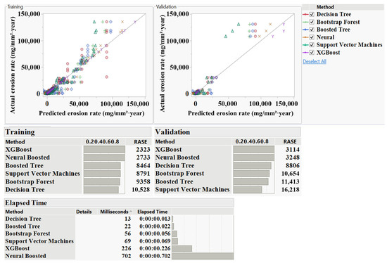
Figure 4. Comparative model screening results to determine the best-performing machine learning algorithm for erosion rate prediction.

In contrast, BT, BF, and DT demonstrated moderate performance with varying degrees of generalisation. BT attained a training RASE of 8464 and experienced a substantial increase to 11,413 in validation, suggesting some degree of overfitting. BF showed stable but modest performance (RASE ≈ 9358 in training and 10,654 in validation), limiting its predictive precision. Interestingly, DT showed a training RASE of 10,528 and an improved validation RASE of 8806, although its error magnitude remained high, suggesting model underfitting during the training phase. Support Vector Machines (SVM) showed the weakest performance overall, with the highest validation RASE (16,218), indicating insufficient capacity to generalise across the erosion dataset. From a computational standpoint, all models executed within milliseconds. XGBoost and Neural models required slightly longer runtimes (226 ms and 702 ms, respectively), but their superior predictive accuracy justified the marginal increase in computational time.

Based on this comparative evaluation, XGBoost and ANN were selected as the leading candidates for further investigation. Subsequent sections of the manuscript examine these models in greater detail, including their predictive diagnostics, error distribution, and interpretability, with the goal of establishing a reliable, interpretable, and generalizable framework for predicting erosion rates under varied environmental and material conditions.

2.3. Artificial Neural Network

ANN algorithm has emerged as a powerful computational framework for modelling complex, nonlinear systems, particularly where interactions among multiple variables are difficult to capture with traditional regression or mechanistic models. Rooted in the structure of biological neural systems, an ANN simulates learning through interconnected layers of artificial neurons, enabling them to adaptively approximate functions and detect hidden patterns in data [36]. Its capabilities have proven valuable in various fields, including engineering, finance, healthcare, environmental science, and numerous others [37,38].

A standard feedforward neural network consists of nodes and connections between the nodes. It has three main parts: an input layer, one or more hidden layers, and an output layer [36,39]. The input layer receives the independent variables. The hidden layers perform the core of the nonlinear transformations. These layers extract complex patterns and interactions through mathematical operations applied at each neuron. All variables of the input layer connect to each neuron of the next hidden layer through weighted connections. Each hidden node computes a weighted sum of its inputs, adds a bias term, and then applies a selected activation function to determine its output. Finally, the output layer consolidates the information and generates a prediction in the form of a continuous numerical value [39].

In the ANN training process, weights and biases are fundamental parameters that determine how information flows through the network and how predictions are made. Each input to a neuron is multiplied by a corresponding weight, which adjusts the strength or importance of that input. The weight essentially tells the network how much influence a given input should have on the output. A higher weight amplifies the input’s effect, while a lower (or negative) weight reduces or reverses it. The bias is an additional parameter, acts as an intercept term, added to the weighted sum of inputs before applying the activation function. It allows the model to shift the activation function to better fit the data. These weights and biases are not fixed; instead, they are learned during training, allowing the network to minimise prediction error and enable the ANN to approximate complex functions and patterns in data with high flexibility [39].

The activation functions are a critical component of the ANN, introducing the non-linearity needed for the network to learn complex patterns and approximate the predicted non-linear functions. The output from each neuron is passed through an activation function before being transmitted to the next layer. Without activation functions, the entire network would reduce to a simple linear transformation [39]. JMP Pro supports up to two hidden layers and allows any combination of three available activation functions, offering flexibility for a wide range of non-linear transformations to suit different modelling contexts. The mathematical expressions of these functions are presented in Table 2.

Table 2. Common activation functions used in ANN modelling.

Activation Function	Mathematical Expression
Hyperbolic Tangent (TanH)	$\phi \left(Z\right)={\displaystyle \frac{e^{2Z}-1}{e^{2Z}+1}}$
Gaussian	$\phi \left(Z\right)=e^{-Z^2}$
Identity (Linear)	$\phi \left(Z\right)=Z$

2.3.1. ANN Mathematical Representation and Model Training

To illustrate the fundamental computational mechanism of the ANN in predicting erosion rate, this section presents a simplified example of the forward propagation process. While the actual architecture implemented in this study involves a larger number of variables and potentially deeper hidden layers, the following formulation captures the essential logic underlying the machine learning process. The network propagates input information through weighted connections, applies bias terms, and transforms the resulting values using activation functions.

As shown in Figure 5, the network structure consists of:

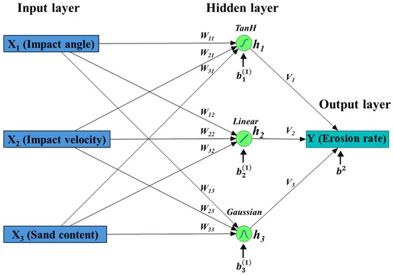
Figure 5. Simplified ANN schematic illustrating the basic structure, layer connectivity, and computational flow involved in predicting erosion rate.

• An input layer comprising three variables: impact angle (X₁), impact velocity (X₂), and sand content (X₃).
• A single hidden layer with three neurons h₁, h₂, and h₃.
• An output layer with one neuron that produces the predicted erosion rate (Y).

Hidden Layer(s)

In the hidden layer, each neuron receives all input variables of the first observation. These inputs are multiplied by their corresponding weights and summed together. A bias term is then added to the resulting value to form the neuron’s net input. This operation is mathematically expressed in Equation (1):

$$Z_j^{\left(1\right)}=\left(\sum _{i=1}^{3\left(0\right)}{W}_{ij}^{\left(1\right)}{X}_i^{\left(0\right)}+b_j^{\left(1\right)}\right)$$

(1)

where

• $Z_j^{\left(1\right)}$: the net input to the hidden neuron j in the first hidden layer.
• $X_i^{\left(0\right)}$: the i-th input variable from the input layer.
• $W_{ij}^{\left(1\right)}$: the weight connecting input variable i to hidden neuron j in the first hidden layer.
• $b_j^{\left(1\right)}:$ the bias term associated with the hidden neuron j in the first hidden layer.

This process allows the network to adjust how strongly each input influences the neuron’s output during training. The net input is then passed through an activation function φ(.) at each hidden neuron j to introduce nonlinearity and get the neuron output (h_j), as shown in Equation (2):

$$h_j^{\left(1\right)}=\phi \left(Z_j^{\left(1\right)}\right)$$

(2)

These outputs are passed (as input variables) to the next layer (either another hidden layer or, in this case, the output layer), and the process (performing a weighted sum of the variables and adding a bias term) is repeated at each neuron of the next layer.

Output Layer

In single-output models, such as erosion rate prediction, the output neuron aggregates the weighted outputs from the neurons of the last hidden layer and adds a bias term to that sum. Since the task involves continuous prediction, a linear (identity) activation function is normally applied at the output layer, enabling the network to generate real-valued outputs [39].

The formulation is expressed in Equation (3).

$$Y=\left(\sum _{j=1}^{3\left(1\right)}{V}_j^{\left(2\right)}{h}_j^{\left(1\right)}+b^{\left(2\right)}\right)$$

(3)

where:

• Y: the predicted erosion rate.
• $V_j^{\left(2\right)}$: the weight connecting the output of hidden neuron j to the neuron of the output layer.
• $h_j^{\left(1\right)}$: the output of hidden neuron j in the hidden layer.
• $b^{\left(2\right)}$: the bias term associated with the output neuron.

Equations (1) and (3) can be generalised for a multilayer neural network with m layers. The output for a neuron j in layer number (L + 1):

$$h_j^{(L+1)}={\phi }_j^{(L+1)}\left(\sum _{i=1}^{n\left(L\right)}{W}_{ij}^{\left(L+1\right)} h_i^{\left(L\right)}+b_j^{\left(L+1\right)}\right)$$

(4)

where n is the total neurons or variables in the previous layer (L). L = 0 for the input layer and L = m − 1 for the output layer.

In the same way, the predicted value in the output layer m:

$$Y=\left(\sum _{j=1}^{n\left(m-1\right)}{V}_j^{\left(m\right)}{h}_j^{\left(m-1\right)}+b^{\left(m\right)}\right)$$

(5)

The same process is repeated for the rest observations in the dataset to calculate their predicted values.

Selecting the Number of Hidden Layers and Nodes

Selecting the optimal number of hidden nodes in an ANN is crucial for achieving the best predictive performance. This number is influenced by several factors, including the size of the dataset, the inherent complexity of the target function, and the level of noise present in the data [12]. An insufficient number of hidden nodes limits the network’s capacity to learn the underlying patterns, often resulting in underfitting. This condition is typically characterised by high error in both training and validation sets, indicating that the model is too simple to represent the data structure effectively. In such cases, increasing the number of hidden nodes may be necessary to enhance the model’s learning capacity. Conversely, using too many hidden nodes can lead to overfitting, where the model captures noise or minor fluctuations in the training data rather than the general pattern. This is commonly observed when the training error is low, but the validation error remains high, suggesting weak generalisation to unseen data. When this occurs, reducing the number of hidden nodes can help restore model balance and improve its ability to generalise [40]. The model performance generally improves with the addition of hidden nodes up to a certain point, beyond which predictive accuracy begins to decline. A practical approach involves starting with a small number of hidden nodes and gradually increasing them while monitoring prediction error through cross-validation. The process should stop once the validation error begins to rise.

Neural networks can be constructed with either one or more hidden layers, depending on the complexity of the modelling task. While a single hidden layer is typically sufficient for most modelling problems, the use of a second hidden layer can substantially reduce the total number of neurons needed [41].

Model Training

Training an ANN involves optimising internal parameters (weights and biases) to minimise the error between the predicted output and the actual target. This is achieved by reducing a loss function, typically the mean squared error (MSE) in regression tasks, which quantifies the prediction accuracy [42]. The training process unfolds in three main steps:

a.

Forward Propagation

At the start of training, the network’s weights and biases are initialised with small random values, providing a neutral starting point. The input data is then passed through the network, layer by layer. Each neuron receives inputs from the previous layer, multiplies them by their respective weights, adds a bias term, and applies an activation function to produce an output. These outputs are propagated forward as inputs to the next layer until reaching the output layer. The final output represents the network’s initial prediction.

b.

Loss Computation

The predicted output is then compared with the true target value using a predefined loss function. The computed loss indicates how far the model is from the expected outcome, guiding the model to adjust its parameters accordingly.

For each observation i, the difference between the measured erosion rate and the network prediction is treated as a residual. The loss function (l) aggregates these residuals and adds a penalty on the network weights to control model complexity [11] (Equation (6)):

$$l={\displaystyle \frac{1}{N}}\sum _{i=1}^N{\left(Y_i-{\mathrm{Ŷ}}_i\right)}^2+\lambda {\parallel W\parallel }^2$$

(6)

where $Y_i$ is the measured erosion rate, ${\mathrm{Ŷ}}_i$ is the ANN prediction, N is the number of samples, ${\parallel W\parallel }^2$ represents the sum of all squared network weights, and λ is the regularisation parameter. The first term represents the deviations between experiments and predictions, while the second penalises large weight magnitudes, effectively controlling model complexity and reducing overfitting to experimental noise. This regularisation term encourages the model to capture the underlying physical relationships rather than spurious fluctuations.

c.

Backpropagation and weight update

After the loss is calculated, the network uses the backpropagation algorithm to determine how each weight and bias contributed to the error. This is done by computing the gradient of the loss function with respect to each parameter, layer by layer, moving backward from the output to the input. These gradients indicate the direction and magnitude of change needed to reduce the error. The weights and biases are then updated in the direction that minimises the loss. This process is repeated iteratively across multiple training cycles, with each cycle nudging the model towards a set of weights and biases that produce a lower prediction error. As the training progresses, the neural network repeatedly updates its parameters to make increasingly accurate predictions. Over time, the SSE becomes smaller, and the network learns the underlying patterns within the training data. To adhere to the principle of parsimony and prevent over-parameterisation, a stopping protocol was employed. The training process was halted when the validation SSE ceased to decrease and began to plateau or rise. This ensures the model captures the underlying physical signal while maintaining robust generalisation performance.

2.4. Extreme Gradient Boosting

XGBoost is an ensemble learning algorithm based on the gradient boosting framework, widely recognised for its exceptional performance in both classification and regression tasks. It constructs a predictive model by iteratively adding weak learners (typically decision trees), each one focusing on minimising the residual errors of prior trees [43]. XGBoost optimises both computation speed and model accuracy through regularisation, parallel processing, and tree pruning techniques, making it a preferred choice for structured data in scientific and industrial applications [44]. XGBoost makes predictions by combining the outputs of multiple decision trees, each one trained to focus on the residuals (the errors) of its predecessor. These trees are built in stages, with each tree refining the overall model’s predictions by learning patterns in the parts where previous models performed poorly. The final prediction is the sum of the outputs from all trees, which collectively approximate the complex function mapping input variables to the output. This strategy ensures that the model continuously improves until a stopping criterion is met, such as a maximum number of trees or a minimal reduction in prediction error.

XGBoost Mathematical Representation and Model Training

a.

Initial prediction and residual computation

To illustrate how XGBoost works in predicting erosion rates, consider a simplified case involving three input features: X₁ (impact velocity, X₂ (impact angle), and X₃ (sand content), as structured in Figure 6. These variables represent key factors influencing erosion behaviour. Suppose we have six samples indexed by i = 1 to 6, where each sample is associated with a measured erosion rate Y_i.

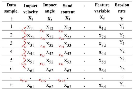
Figure 6. Structure of the input feature matrix for XGBoost, illustrating n samples and d features (from X₁ to X_d). Threshold values c represent candidate split points evaluated between successive feature values during tree construction. Red arrows mark candidate split points; dots indicate continuation for more samples or features.

XGBoost starts by assigning a base prediction for all samples. This base value is typically the mean of the target variable (erosion rates). So, the initial output prediction for all data samples:

$${\mathrm{Ŷ}}_i^{\left(0\right)}=Ȳ={\displaystyle \frac{1}{n}}\sum _{i=1}^n{Y}_i$$

(7)

where:

• ${\mathrm{Ŷ}}_i^{\left(0\right)}$: the initial prediction for sample i.
• Y_i: the observed erosion rate for sample i.
• n: the number of samples.

Based on this initial prediction, the first residual $\left(r_i^{\left(1\right)}\right)$ is calculated for each data point i as the difference between the actual and predicted values:

$$r_i^{\left(1\right)}=Y_i-{\mathrm{Ŷ}}_i^{\left(0\right)}$$

(8)

These residuals serve as the learning target to build the first regression tree.

b.

Boosting iteration (tree by tree training)

The XGBoost model is trained by minimising a regularised objective function that combines a squared error measure of fit with a penalty on tree complexity [43]. The overall prediction is the sum of the contributions from all trees, and the objective function takes the standard form, as given in Equation (9):

$$Obj=\sum _{i=1}^N{\left(Y_i-{\mathrm{Ŷ}}_i\right)}^2+\sum _{k=1}^K\Omega \left(f_k\right)$$

(9)

where $Y_i$ and ${\mathrm{Ŷ}}_i$ are the actual and predicted erosion rates, K is the number of trees, and Ω(f_k) is the regularisation term for each individual tree. This term includes penalties on the number of leaves and the magnitude of leaf weights, typically expressed as shown in Equation (10):

$$\mathit{\Omega }\left(f\right)=\gamma T+{\displaystyle \frac{1}{2}}\lambda \sum _{j=1}^T{W}_j^2$$

(10)

Here, T is the number of leaves in a tree, W_j is the weight assigned to the jth leaf, λ controls weight regularisation, and γ penalises tree complexity [43,44,45]. The squared-error term measures how well the ensemble fits the data, while the tree and weight-penalty terms restrict unnecessary splits and extreme leaf outputs, preventing the model from adapting to isolated, noisy observations, overfitting and improving generalisation.

To minimise this objective function efficiently, XGBoost employs a greedy algorithm that iteratively adds branches by selecting the split that provides the maximum reduction in the objective function.

During the training of each tree, starting from the root and at each subsequent node creation step, XGBoost evaluates every single feature (in this case, X₁, X₂, and X₃) and considers all potential split thresholds, typically the midpoints between adjacent sorted unique values (as illustrated in Figure 6, for thresholds c₁₁ to c₅₃). It uses the exact greedy algorithm to choose the optimal pair (feature, split threshold) that maximises a metric called gain, which measures the reduction in loss function resulting from the split. The algorithm always selects the split with the highest gain at each node and proceeds with a split only if it improves the prediction accuracy. This is what makes the algorithm greedy in the split process [45]. The gain for a proposed split is calculated as follows:

$$Gain={\displaystyle \frac{1}{2}} \left[{\displaystyle \frac{{\left({\sum }_{i\in I_L}{g}_i\right)}^2}{{\sum }_{i\in I_L}{h}_i+\lambda }}+{\displaystyle \frac{{\left({\sum }_{i\in I_R}{g}_i\right)}^2}{{\sum }_{i\in I_R}{h}_i+\lambda }}-{\displaystyle \frac{{\left({\sum }_{i\in I}{g}_i\right)}^2}{{\sum }_{i\in I}{h}_i+\lambda }}\right]-\gamma$$

(11)

where:

• g_i: the first-order gradient of the loss function = − residual (r_i).
• h_i: the second-order gradient of the loss function = 1.
• λ: the regularisation term, penalises complexity (trees with many leaves or large values).
• γ: the minimum gain threshold required to make a split.
• I, I_L, I_R: the sample sets for node, left child node, and right child node.

As shown in Figure 7, the first tree is trained on the initial residuals and attempts to reduce the error by optimally partitioning the input space. For example, the root node may split on impact velocity X₁ ˂ c₁₁ if this gives the highest gain, and that becomes the first split in this tree. After splitting the calculated residuals and forming left and right child nodes, this process continues iteratively for each branch, and different features may be selected at different depths or nodes. In the right child node, XGBoost may choose X₂ ˂ c₃₂ as the best next split, so the impact angle is used at the second level. However, no further splitting process can be applied to the left child node, as it has only one residual value. So, each branch can explore different features, depending on how useful each is for prediction. This process allows XGBoost to efficiently utilise multi-dimensional feature interactions and capture complex relationships between the input variables and the target.

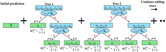
Figure 7. Simplified XGBoost schematic illustrating sequential tree construction and boosting process: the first tree is trained to minimise initial residuals. The second tree is added to refine the prediction by learning from remaining errors. Each tree incrementally refines the prediction function. Arrows indicate the flow of the boosting process and the direction of tree construction; dots represent continuation for additional trees.

c.

Checking the stopping criteria

The XGBoost tree continues to make nodes and goes deeper until one or more stopping criteria are met. These are summarised in Table 3.

Table 3. Stopping criteria used by XGBoost during tree construction.

Conditions	Description
Maximum depth	Maximum number of levels per tree.
Minimum number of residuals	Minimum number of sample residuals required per child node.
γ	Minimum gain required to make a split.
No gain improvement	Branches are pruned if no gain is achieved.
No more samples to split	Nodes with ≤1 sample are not split further.

d.

Making leaf nodes

Once no further progress is applicable and the tree structure is finalised, XGBoost creates leaf nodes and assigns a weight value for each leaf as the tree output for any sample i that falls into that leaf. This value represents a corrective term that updates the previous prediction. The optimal weight for a leaf j of the first tree is given by:

$${f^{\left(1\right)}\left(x_i\right)=W}_j^{\left(1\right)}=- {\displaystyle \frac{{\sum }_{i\in I_j}{g}_i}{{\sum }_{i\in I_j}{h}_i+\lambda }}$$

(12)

where I_j denotes the set of samples in leaf j.

e.

Updating the predictions

Each sample’s predicted value is then updated by adding the weighted output W_j of the leaf where the sample’s residual falls, scaled by a learning rate.

$${\mathrm{Ŷ}}_i^{\left(1\right)}={\mathrm{Ŷ}}_i^{\left(0\right)}+\eta .f^{\left(1\right)}\left(x_i\right)$$

(13)

The learning rate (η), also referred to as shrinkage, controls how much each tree contributes to the overall predictive model by scaling its newly added weights at each boosting iteration. A smaller η promotes gradual learning and better generalisation by reducing the impact of each tree, while a larger η accelerates convergence but increases the risk of overfitting [43].

f.

Adding the second tree

After updating the predicted values, a new set of residuals is computed by calculating the difference between the actual targets and the latest predictions, forming the basis for training the subsequent tree:

$$r_i^{\left(2\right)}=Y_i-{\mathrm{Ŷ}}_i^{\left(1\right)}$$

(14)

The second tree is then trained on these residuals using the same procedure. The algorithm re-evaluates all available features and potential split points to identify the optimal (feature, threshold) pair that reduces the loss [44]. As illustrated in Figure 7, the best first split may occur on feature X₂ at threshold c₃₂, followed by subsequent splits for both branches on X₃ at c₅₃ and X₁ at c₂₁, effectively partitioning the residuals to refine the prediction.

The structure of each tree can differ depending on the data and the splitting criteria used to reduce loss. Some trees may be deeper, while others are shallower. Within a single tree, certain branches can extend further than others, highlighting variations in the splitting process at each level.

g.

Iterative ensemble construction

This process continues iteratively, adding more trees to the ensemble. Each new tree $f^{\left(k\right)}$ is trained on the latest residuals to minimise the overall loss. After K trees, the final prediction for sample i is the cumulative output of all trees, as expressed in Equation (15):

$${\mathrm{Ŷ}}_i^{\left(K\right)}={\mathrm{Ŷ}}_i^{\left(0\right)}+ \eta .\sum _{k=1}^K{f}^{\left(k\right)}\left(x_i\right)$$

(15)

Training concludes when either a predefined number of trees is reached (see ‘iterations’ in Table 4) or when no further improvement in the validation loss is observed [43]. Aligning with the principle of parsimony, this optimised stopping mechanism prevents over-parameterisation by halting the additive process early enough to prevent the model from overfitting. Consequently, this allows XGBoost to progressively refine its predictions and deliver high predictive performance while maintaining robust generalisation.

Table 4. XGBoost hyperparameters and their default values.

Hyperparameter	Default Value	Function and Explanation
max_depth	6	Determines the maximum depth of each tree in the ensemble. Deeper trees model more complex relationships but can also lead to overfitting.
subsample	1	Fraction of training samples used for each boosting round; reduces variance and overfitting when set below 1.
colsample_bytree	1	Fraction of predictors randomly selected for each tree; this setting can improve learning capacity; however, it can mitigate multicollinearity when set below 1.
min_child_weight	1	Minimum sum of instance weights required to create child nodes (leaf). Setting it to 1 allows the model to capture even rare patterns or fine shifts in the input data.
alpha	0	Regularisation term. Controls model sparsity by penalising the absolute values of leaf weights; helps remove weak tree branches and simplifies the model.
lambda	1	Regularisation term. Controls model complexity by penalising large leaf weights; stabilises the tree structure and reduces overfitting to noisy data.
learning_rate	0.3	Shrinkage parameter. Controls the contribution of each tree to the final prediction; lower values slow learning but improve accuracy.
iterations	30	Number of boosting rounds (trees built); more iterations can capture complexity but risk overfitting.

2.5. Model Validation and Performance Assessment

Following the training phase, it is essential in both algorithms to validate the model’s ability to generalise beyond the training data. This process assesses whether the network has learned meaningful patterns or merely memorised the training data, resulting in weak predictive performance outside the training set. In this study, K-fold cross-validation is employed to ensure a reliable and unbiased evaluation of the model. The dataset is randomly partitioned into (K = 5) equally sized subsets (folds). The model training process is repeated K times. In each iteration, four folds (K − 1) are used for training, and one is strictly held out as a validation set. This ensures that every data point serves as a validation set exactly once without any overlap within each run. It also reduces model dependency on any single data partition, providing a robust model performance that is less sensitive to the randomness of a single data split. This approach was selected instead of using a separate test because it maximises data utilisation and gives effective results even with small or noisy datasets [11]. While a held-out test set can provide an independent measure of model accuracy, cross-validation is a widely accepted method for robust predictive accuracy [35].

2.6. Machine Learning Modelling Procedure in JMP Pro

This section outlines the detailed procedures for initiating and launching ANN and XGBoost algorithms in JMP Pro. Each method was configured through its interactive interface to build and validate predictive models for estimating erosion rates. The configuration process includes selecting input variables, defining model settings, and preparing the platforms for the subsequent modelling process.

2.6.1. ANN Modelling in JMP Pro

To initiate a neural network model in JMP Pro, users begin by accessing the “Neural” platform from the “Analyse” menu, followed by selecting erosion rate as the (Y) response and erosion variables as the (X) factors. Once the variables are assigned, the “Model Launch” window (Figure 8) will appear, allowing for full customisation of the model’s structure, validation method, and training settings. The first step in setting up the model involves specifying the Validation Method. JMP Pro 18 supports various validation techniques. “K-Fold” is selected, which divides the dataset into k subsets (folds), here set to 5 folds, for iterative training and validation. The “Random Seed” field allows users to specify a fixed seed value, ensuring the reproducibility of results. If left at the default value of zero, the seed changes with each run, resulting in non-reproducible outcomes that can cause variation in model performance metrics and hinder the ability to validate or compare results across different runs.

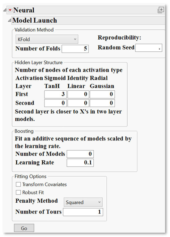
Figure 8. ANN model launch panel in JMP Pro, showing settings for validation, hidden layer structure, and boosting configuration.

Next, users define the “Hidden Layer Structure”, which shapes the neural network architecture. JMP Pro offers three activation function options: “TanH”, “Linear”, and “Gaussian”. In the default configuration shown, the first hidden layer includes three “TanH” nodes, and the second layer

Remains empty, indicating a single-layer neural network. Adding a second layer enables deeper representations, which are particularly useful for capturing complex nonlinear interactions. The Boosting section is an optional enhancement that allows the user to fit a sequence of models where each subsequent model learns from the errors of the previous one. Boosting is controlled by the “Number of Models” and “Learning Rate” parameters. Although these values are set to zero and 0.1, respectively, in the default view, users can adjust them to apply learning techniques that often improve predictive performance [35].

Under Fitting Options, JMP offers further optional refinements. Selecting Transform Covariates enables automated data transformations, which can enhance model interpretability and performance. The Robust Fit option increases resistance to the influence of outliers. The Penalty Method “Squared” helps prevent overfitting by penalising large weights. Lastly, the Number of Tours specifies how many times the fitting process is repeated, each time with different random initial parameter values. The model with the best validation statistic and the lowest prediction error across all tours is selected. Once all parameters are appropriately configured, clicking the “Go” button initiates the model training process.

2.6.2. XGBoost Modelling in JMP Pro

The XGBoost platform is not available by default in JMP Pro 18 and must be manually installed as an official Add-In provided by JMP’s extension community. Once installed, it appears under the “Add-Ins” tab in the JMP toolbar. Before training the XGBoost model, it is necessary to generate K-fold cross-validation columns. This was accomplished by navigating to (Add-Ins > XGBoost > Make K-Fold Columns), where the Erosion rate variable was selected for both the “Y-Response” and “Stratify By” fields to maintain balanced fold distribution. Using the default settings, three validation columns (Fold A, Fold B, and Fold C) were created with K = 5, enabling repeated K-fold analysis. These fold columns were then assigned as validation variables during model setup (Add-Ins > XGBoost > XGBoost), while erosion variables were defined as predictors. This configuration ensures that each subset of the data is used both for training and validation across multiple rounds, enhancing the robustness and generalisability of the model. Once the validation columns are assigned and the predictors selected, clicking “OK” opens the XGBoost launch window (Figure 9), where model configuration and training parameters are specified.

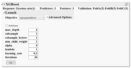
Figure 9. XGBoost launch interface in JMP Pro, where core hyperparameters and advanced model settings are defined prior to training.

This window allows users to specify core hyperparameters that govern tree construction and learning behaviour. On the left-hand side, several key parameters are displayed with their default or user-defined values. Table 4 below summarises the primary hyperparameters available for XGBoost, along with their functions and implications for model performance.

“Autotune” feature optimises hyperparameters through internal validation, enhancing model performance with minimal manual input. For greater control, the “Advanced Options” panel provides access to settings such as booster type, objective function, and tree construction strategy, allowing fine-tuning to match data complexity [35]. Once the appropriate settings are selected, clicking “Go” initiates the training and validation processes.

3. Results and Discussions

3.1. ANN Model Development

To identify the optimal ANN structure for predicting erosion rates, several trials were conducted to evaluate different combinations and distributions of activation functions across the hidden layers. These trials aimed to enhance the model’s ability to capture complex, nonlinear interactions among multiple input variables while also ensuring generalisation to unseen data. The final design was selected after comparing multiple configurations using the modelling performance metrics.

The model employed a two-hidden-layer feedforward structure. As illustrated in Figure 10, the first hidden layer comprised 20 neurons, evenly split between “TanH” and “Gaussian” activation functions. This number and hybrid configuration were intentionally adopted to maximise the network capacity for learning nonlinear patterns across the diverse dataset. The justification for this arrangement is supported by the specific characteristics of each activation function. The “TanH” functions are effective in representing symmetrical and continuous dependencies [46], particularly those arising from physical test conditions such as velocity and angle variations. In contrast, the “Gaussian” functions are introduced to increase the network sensitivity to localised patterns and abrupt transitions in the data [47], such as those arising from variations in polymer type or fluid composition. The second hidden layer comprises five linear activation nodes, primarily serving as a feature aggregator. This linear stage simplifies the high-dimensional transformations produced by the first layer, stabilises the training process, and enhances model generalisation [12].

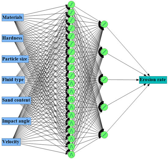
Figure 10. Schematic of the developed ANN predictive model for erosion rate in polymers and composites, featuring seven input variables, two hidden layers, and one output node. Circles represent neurons; arrows indicate the direction of information flow.

3.2. XGBoost Model Development

The XGBoost model used in this study has seven predictors and a total of sixteen engineered features. Cross-validation was applied using three-fold columns (Fold A, Fold B, and Fold C), each consisting of five partitions, to ensure reliable performance estimation and reduce the risk of overfitting. To ensure optimal predictive performance and model stability, the XGBoost algorithm was configured using the Autotune feature. This function systematically explores combinations of hyperparameters within a predefined search space using internal cross-validation, selecting the configuration that offers the best generalisation performance.

Figure 11 illustrates the XGBoost full launch interface, which includes the predefined minimum and maximum boundaries assigned to each hyperparameter, as well as the optimal values selected through the tuning process. The effectiveness of this optimisation is reflected in the iteration history plot on the right, which visualises the training and validation error curves (objective metric: root mean square error) over the boosting iterations.

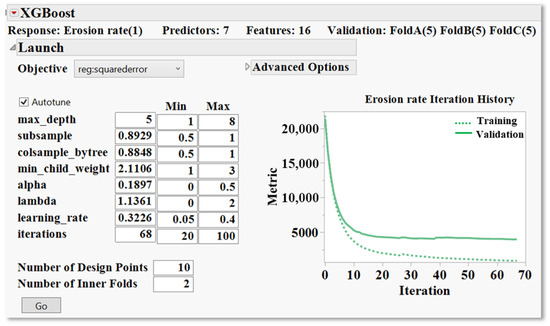
Figure 11. XGBoost launching interface in JMP Pro 18, displaying the model configuration and training results, including optimised hyperparameter values, the minimum and maximum parameter boundaries used during tuning, and the convergence history for training and validation errors.

Both curves exhibit a steep error reduction during the early iterations, followed by a gradual levelling off as the model convergence is approached. This early-stage gradient confirms that the model quickly learns the most influential patterns in the data, whereas the gradual flattening in later iterations reflects the model’s convergence, indicating a well-regularised boosting process where additional trees contribute progressively less to predictive improvement. Notably, the gap between the training and validation curves remains narrow and consistent throughout the learning process. This reflects a well-balanced model that captures the system’s complexity without overfitting. The absence of an upward trend in the validation curve during the later iterations, which would typically indicate overtraining or excessive model complexity, confirms that the selected hyperparameter configuration provided sufficient regularisation and ensured stable learning. This type of learning curve behaviour aligns with best practices observed in high-performing XGBoost models applied to nonlinear systems [14].

3.3. Model Performance Comparison of ANN and XGBoost

The predictive capabilities of the XGBoost and Artificial Neural Network (ANN) models were closely evaluated to identify the optimal framework for forecasting erosion rates. The assessment utilised multiple statistical metrics, focusing on the correlation coefficient (r), the Root Average Squared Error (RASE), and Mean Absolute Error (MAE), complemented by actual versus predicted response plots for both training and validation phases (see Table 5 and Figure 12). During the training phase, both models demonstrated exceptional performance, with r values of 0.999 for XGBoost and 0.993 for ANN. However, XGBoost achieved lower error metrics (RASE = 861; MAE = 448) compared to ANN (RASE = 2047; MAE = 1216). This suggests that XGBoost aligns more closely with the training dataset. While such tight fitting may reflect robust learning, it can also raise concerns about potential overfitting. However, the training process was strictly halted when validation performance ceased to improve, ensuring that the model did not overfit.

Table 5. Performance evaluation of erosion rate prediction using ANN and XGBoost.

Measures	ANN Fit Details		XGBoost Fit Details
	Training	Validation	Training	Validation
r	0.993	0.999	0.999	0.990
RASE	2047	1159	861	3760
MAE	1216	652	448	1815

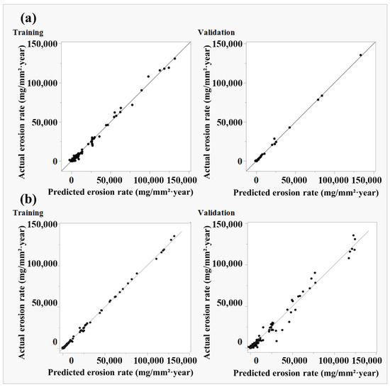
Figure 12. Actual vs. predicted erosion rates for both training and validation phases: (a) ANN and (b) XGBoost.

The validation phase revealed clear differences between the two models. The ANN model achieved a higher r of 0.999, outperforming XGBoost’s r of 0.990. More critically, ANN exhibited significantly lower predictive errors (RASE = 1159; MAE = 652) compared to XGBoost (RASE = 3760; MAE = 1815). This marked disparity underscores the superior ability of ANN to generalise to unseen data. Visual analysis of the prediction scatterplots provides further support for this conclusion: ANN predictions closely align with the 1:1 reference line, demonstrating minimal bias and consistent performance across the entire erosion rate spectrum. In contrast, XGBoost predictions show increased dispersion in high-erosion regimes, indicating reduced reliability under extreme conditions. Although the RASE and MAE values for both models may appear substantial, they are relatively modest compared to the maximum erosion rates observed in the collected dataset, which can exceed 130,000 mg/(mm²·year) under high-velocity, high-sand conditions.

Based on this comparative analysis, the ANN model is identified as the more reliable and effective predictive tool for forecasting erosion rates. While XGBoost slightly outperformed in training, ANN’s performance was significantly better in validation. Its consistently high r, lower predictive errors, and stable performance across diverse erosion scenarios demonstrate its superior generalisation capabilities. These attributes make it the preferred choice for forecasting erosion rate in this study.

3.4. Validating Model Interpretability and Physical Consistency

To better understand the performance of the developed models in representing the individual and combined effects of input variables on the predicted erosion rate, a prediction profiler analysis was generated using the trained ANN and XGBoost models. This tool provides a visual and interpretable representation of the model’s predicted response to a controlled change in each input factor while holding others constant. This analysis enables a critical evaluation of the model’s internal structure and learned variable interactions for physical interpretability by allowing for an interactive examination and comparison of predicted trends with established physical behaviours observed in the erosion literature, thereby validating the model’s physical credibility. The upper part of Figure 13 illustrates the effect of the seven predictors on the erosion rate using both ANN and XGBoost models. The vertical red dashed lines represent the selected scenario values, while the black trend lines depict the model’s predicted response across each variable’s range.

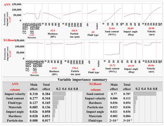
Figure 13. Prediction profiler curves and variable importance analyses for ANN and XGBoost models. Profiles illustrate the effect of each input variable on predicted erosion rate; bar charts compare the main and total effects across models.

ANN profiler reveals differentiated erosion responses across the materials investigated, with some fibre-reinforced composites showing higher predicted erosion rates compared with certain unfilled polymers. Erosion behaviour in composites is mainly governed by the properties of the fibre and matrix, the integrity of the fibre–matrix interface, and the orientation and distribution of the reinforcement. In cases of weak interfacial adhesion, brittle matrices, or unfavourable fibre alignment, impact loading can lead to matrix cracking, fibre exposure, and interfacial debonding, resulting in accelerated surface degradation [48]. In contrast, certain unfilled polymers may resist erosion more effectively due to energy absorption, elastic recovery, and smoother deformation-driven wear, leading to lower material loss under similar conditions. Previous studies have shown that neat polymers can outperform some composites in comparable erosive environments [23,24,31,49,50]. These trends were clearly reflected in the ANN output but appeared largely absent in the XGBoost profiler, where erosion rate predictions remained nearly flat across most materials, suggesting limited sensitivity to compositional differences.

The surface hardness curve in the ANN model shows a mild decreasing trend in erosion rate with increasing hardness, supporting the general understanding that harder surfaces are more resistant to erosion [5,51]. Unlike ANN, the XGBoost model displayed a step-like profile for hardness, with minimal incremental slope variation. For particle size, both models capture the expected positive trend, with the erosion rate increasing as the particle size increases. This is consistent with experimental findings attributing higher erosive damage to the greater momentum and impact energy of larger particles [5,51]. However, ANN delivered a smoother, more continuous curve, whereas XGBoost showed abrupt transitions. A similar contrast was observed in the sand content variable. ANN profile exhibits a nonlinear increase in erosion rate, with a steep initial rise that gradually levels off at higher concentrations. This response is likely due to increased particle–particle interactions, such as collisions between incoming and rebounding particles, which dissipate kinetic energy and reduce the effective impact on the surface [5]. XGBoost profiler displayed a more abrupt and segmented curve. This step-like trend results from the model’s reliance on decision-tree partitioning. XGBoost builds predictions by dividing the input space into discrete regions and applying constant outputs within each partition. This leads to abrupt transitions in the prediction surface, rather than smooth and continuous responses [43,52]. The fluid type effect in the ANN profiler accurately captures the enhanced erosion in slurry systems compared to dry conditions. In addition to erosion caused by water impact itself [26,31], solid particles entrained by water have higher impact energy due to water’s higher density and viscosity, which enhances the drag force and momentum transfer [51,53]. XGBoost response was unable to distinguish between dry and wet erosion. The impact angle response follows the expected semi-ductile pattern, with maximum erosion occurring at intermediate angles due to the combined effects of normal and tangential forces [23,24,25,50]. The ANN model captured this peak distinctly, whereas the XGBoost output appeared flatter and less responsive to angular changes. Finally, the ANN velocity curve shows a pronounced upward trajectory, consistent with the widely reported velocity exponent effect in erosion wear, where erosion rate scales sharply with increasing impact speed [5,7,54,55,56,57,58]. Higher impact velocities result in a greater transfer of kinetic energy to the surface, intensifying the erosive action and accelerating material loss [5,59,60]. XGBoost profiler showed a relatively compressed slope, underestimating the velocity sensitivity in higher ranges.

The outcomes of profiler analysis confirm that the ANN model has not only learned statistical patterns but also effectively captured the underlying erosion mechanisms across a complex, multivariable input domain. The model predictions closely align with the established physical trends in the literature, validating its reliability as a predictive tool for erosion behaviour. Several studies support the effectiveness of ANN in resolving complex erosion predictive modelling [15,18,21,61]. By contrast, while XGBoost can deliver good predictive accuracy, its profiler reveals structural limitations in representing erosion behaviour. A recent study by Brown et al. [62] reported the same limitation of tree-based models, noting that partial dependence plots exhibited step-like profiles due to XGBoost’s discrete splitting. These abrupt jumps and plateaus can misrepresent smooth physical relationships.

The interpretation provided by the prediction profiler is further supported by the variable importance analysis. The ANN model identifies velocity, sand content, and fluid type as the most influential predictors, consistent with well-established erosion mechanisms. In contrast, XGBoost concentrates a greater share of importance on a single variable, with comparatively reduced weighting across the remaining factors.

3.5. Model Export for Deployment

The final stage of the predictive modelling process involved preparing the model for use outside the JMP Pro environment, thereby extending its practical reach beyond the original analytical platform. To facilitate this, the trained model was exported into Python code using JMP Pro’s Formula Depot, preserving all mathematical relationships, variable transformations, and parameter values into executable code required for prediction outcomes. This was achieved by publishing the finalised model to the Formula Depot using the “Publish Prediction Formula” option. Once added, the Formula Depot interface listed the prediction formula, from which Python code was generated using the “Generate Python Code” option. This resulted in a script file “Neural_Erosion_rate.py” that encapsulates the model’s scoring logic. This generated script file, along with a support file “jmp_score.py”, enables standalone execution in a standard Python environment [35].

While the practical application of the exported script in an external system was beyond the scope of this study, the resulting Python code can be used to score new datasets, offering prediction performance consistent with that observed in JMP. This capability enhances the model’s practical applicability, laying the foundation for future operational integration in Python-based data analysis.

4. Conclusions

This study successfully developed and validated a comprehensive data-driven predictive framework for estimating erosion rates in polymers and polymer composites using machine learning algorithms within the JMP Pro platform.

A comprehensive dataset comprising 186 erosion test cases was compiled from peer-reviewed literature and refined through outlier removal, unit normalisation, and exploratory analyses to ensure robustness and consistency. Key input parameters, including impact angle, velocity, sand content, particle size, material type, hardness, and fluid medium, were incorporated to capture the complex nonlinear interactions governing the erosive wear process.

Initially, a model screening process evaluated six widely used algorithms, including XGBoost, ANN, BF, BT, DT, and SVM. ANN and XGBoost were identified as the superior performers based on their excellent predictive accuracy and generalisation abilities.

ANN exhibited superior generalisation capabilities, with a validation r of 0.999, RASE of 1159 and MAE of 652, outperforming XGBoost’s validation metrics of r = 0.990, RASE = 3760 and MAE = 1815. Both models demonstrated strong training fits; however, the ANN provided lower predictive errors and more reliable performance across diverse erosion conditions, underscoring its efficacy in capturing multivariable dependencies. Interpretability analyses, conducted through prediction profilers and variable importance rankings, clearly validated the ANN model’s alignment with established physical erosion mechanisms widely reported in the literature. Key influential variables such as impact velocity, sand content, and fluid medium were accurately reflected through smooth and realistic response curves, reinforcing the model’s reliability and physical credibility. XGBoost, while effective, showed constraints in smoothly depicting continuous variable influences.

The machine learning models developed in this study used five-fold cross-validation to partition the data and evaluate model performance across independent validation sets, providing a realistic estimate of generalisation error. Jackknife distance was applied to detect and remove outliers, protecting the model from anomalous or noisy data points. Residual-based metrics, such as RASE and MAE were calculated on the validation data to quantify prediction accuracy and spread. XGBoost incorporated regularisation terms and tree pruning to reduce overfitting, while ANN models were regularised through architecture control and nonlinear activation functions that smoothed input response. Crucially, both algorithms employed an optimised stopping protocol based on validation error reduction, ensuring that training ceased before the models could overfit to experimental noise. Lastly, prediction profiler tools in JMP were used to examine how each input variable influenced the predicted erosion rate. These profiler trends in ANN followed known physical erosion behaviour, reinforcing the validity and interpretability of the models. This combined approach is well-suited for capturing complex erosion mechanisms under experimental variability.

The optimised ANN model was exported as executable Python code ready for deployment outside the original software environment. This facilitates integration into diverse analytical platforms, thereby extending the model’s practical utility and supporting broader application scenarios.

While this study represents a significant advancement in predictive erosion modelling, it acknowledges limitations such as reliance on literature-derived experimental data. In addition, excluding outliers, particularly those with extreme impact velocities and sand contents, was essential for model stability; however, this also limits the boundaries within which the framework can be applied. Finally, although the models provide accurate predictions, they are unable to prove definitive cause-and-effect relationships between input variables and erosion behaviour, which is beyond the scope of this study. Future research should expand dataset diversity, incorporate real-time operational data, and extend the framework to predict other tribological properties, thereby providing deeper insight and interpretability.

In parallel, where larger datasets permit, the inclusion of a separately held-out test set prior to model training could serve as an additional layer of validation, complementing cross-validation and further supporting the generalisability of the predictive modelling process.

Furthermore, future work may also explore the development of a fully statistical model that explicitly defines variables, assumptions and the stochastic nature of the output and input variables. Such models could offer a complementary statistical perspective to the current machine learning framework by providing deeper statistical insight into the erosion behaviour of polymeric and composite systems.

Overall, this study makes a significant contribution to the predictive modelling field by establishing a validated, interpretable, and deployable erosion prediction framework with considerable potential for practical applications in industries such as aerospace, marine, and energy. It can support lifecycle prediction of polymer-based components in erosive environments, assist in selecting materials with enhanced durability, and contribute to sustainability initiatives by helping to mitigate microplastic generation from eroded polymers. These applications underscore the broader value of the model in guiding material design and management strategies across industrial and environmental contexts.

References

- Rubino, F.; Nisticò, A.; Tucci, F.; Carlone, P. Marine application of fiber reinforced composites: A review. J. Mar. Sci. Eng. 2020, 8, 26. [Google Scholar] [CrossRef]
- Rajak, D.K.; Pagar, D.D.; Menezes, P.L.; Linul, E. Fiber-reinforced polymer composites: Manufacturing, properties, and applications. Polymers 2019, 11, 1667. [Google Scholar] [CrossRef]
- Friedrich, K. Erosive wear of polymer surfaces by steel ball blasting. J. Mater. Sci. 1986, 21, 3317–3332. [Google Scholar] [CrossRef]
- Ruff, A.; Ives, L. Measurement of solid particle velocity in erosive wear. Wear 1975, 35, 195–199. [Google Scholar] [CrossRef]
- Hutchings, I.; Shipway, P. Tribology: Friction and Wear of Engineering Materials; Butterworth-Heinemann: Oxford, UK, 2017. [Google Scholar]
- Bitter, J.G.A. A study of erosion phenomena part I. Wear 1963, 6, 5–21. [Google Scholar] [CrossRef]
- Finnie, I. Erosion of surfaces by solid particles. Wear 1960, 3, 87–103. [Google Scholar] [CrossRef]
- Oka, Y.I.; Okamura, K.; Yoshida, T. Practical estimation of erosion damage caused by solid particle impact: Part 1: Effects of impact parameters on a predictive equation. Wear 2005, 259, 95–101. [Google Scholar] [CrossRef]
- Banazadeh-Neishabouri, N.; Shirazi, S.A. Development of erosion equations for Fiberglass Reinforced Plastic (FRP). Wear 2021, 476, 203657. [Google Scholar] [CrossRef]
- Anderson, K.; Karimi, S.; Shirazi, S. Erosion testing and modeling of several non-metallic materials. Wear 2021, 477, 203811. [Google Scholar] [CrossRef]
- Hastie, T.; Tibshirani, R.; Friedman, J. The Elements of Statistical Learning: Data Mining, Inference, and Prediction; Springer Series in Statistics; Springer: New York, NY, USA, 2009. [Google Scholar]
- Klimberg, R. Fundamentals of Predictive Analytics with JMP; SAS Institute: Cary, NC, USA, 2023. [Google Scholar]
- JMP Statistical Discovery LLC. JMP® Pro, version 18.0.2; JMP Statistical Discovery LLC: Cary, NC, USA, 2024.
- Yu, C.H.A. Data Mining and Exploration: From Traditional Statistics to Modern Data Science; CRC Press: Boca Raton, FL, USA, 2022. [Google Scholar]
- Zhang, Z.; Barkoula, N.-M.; Karger-Kocsis, J.; Friedrich, K. Artificial neural network predictions on erosive wear of polymers. Wear 2003, 255, 708–713. [Google Scholar] [CrossRef]
- Banazadeh-Neishabouri, N.; Shirazi, S.A. Erosive Wear Behavior of Fiberglass Reinforced Plastic Composite and Polyethylene. In Proceedings of the ASME-JSME-KSME 2019 8th Joint Fluids Engineering Conference (AJKFluids2019), San Francisco, CA, USA, 28 July–1 August 2019. [Google Scholar]
- Mahapatra, S.; Satapathy, A. Erosion wear response of ramie-epoxy composites using artificial neural network integrated with Taguchi technique. Mater. Werkst. 2023, 54, 871–882. [Google Scholar] [CrossRef]
- Antil, S.K.; Antil, P.; Singh, S.; Kumar, A.; Pruncu, C.I. Artificial neural network and response surface methodology based analysis on solid particle erosion behavior of polymer matrix composites. Materials 2020, 13, 1381. [Google Scholar] [CrossRef]
- Deliwala, A.A.; Dubey, K.; Yerramalli, C.S. Predicting the erosion rate of uni-directional glass fiber reinforced polymer composites using machine-learning algorithms. J. Tribol. 2022, 144, 091707. [Google Scholar] [CrossRef]
- Mahapatra, S.K.; Satapathy, A. Development of machine learning models for the prediction of erosion wear of hybrid composites. Polym. Compos. 2024, 45, 7950–7966. [Google Scholar] [CrossRef]
- Mahapatra, S.K.; Satapathy, A. Erosion wear performance of titania filled ramie-epoxy composites: A data driven optimization study using supervised machine learning approach. J. Elastomers Plast. 2024, 57, 189–214. [Google Scholar] [CrossRef]
- Roh, Y.; Heo, G.; Whang, S.E. A survey on data collection for machine learning: A big data-ai integration perspective. IEEE Trans. Knowl. Data Eng. 2019, 33, 1328–1347. [Google Scholar] [CrossRef]
- Harsha, A.; Jha, S.K. Erosive wear studies of epoxy-based composites at normal incidence. Wear 2008, 265, 1129–1135. [Google Scholar] [CrossRef]
- Qian, D.; Bao, L.; Takatera, M.; Kemmochi, K.; Yamanaka, A. Fiber-reinforced polymer composite materials with high specific strength and excellent solid particle erosion resistance. Wear 2010, 268, 637–642. [Google Scholar] [CrossRef]
- Patnaik, A.; Satapathy, A.; Mahapatra, S.S.; Dash, R.R. A modeling approach for prediction of erosion behavior of glass fiber–polyester composites. J. Polym. Res. 2008, 15, 147–160. [Google Scholar] [CrossRef]
- Mendoza Mendoza, J.C.; Vera Cardenas, E.E.; Lewis, R.; Mai, W.; Avila Davila, E.O.; Martínez Pérez, A.I.; Ledesma Ledesma, S.; Moreno Rios, M. Water jet erosion performance of carbon fiber and glass fiber reinforced polymers. Polymers 2021, 13, 2933. [Google Scholar] [CrossRef]
- Barkoula, N.-M.; Karger-Kocsis, J. Effects of fibre content and relative fibre-orientation on the solid particle erosion of GF/PP composites. Wear 2002, 252, 80–87. [Google Scholar] [CrossRef]
- Vera-Cardenas, E.E.; Mendoza-Mendoza, J.C.; Martinez-Perez, A.I.; Ledesma-Ledesma, S.; Rubio-González, C.; Vite-Torres, M. Solid particle erosive wear study of polymer composite materials for wind turbine applications. Polym. Compos. 2021, 42, 1988–1999. [Google Scholar] [CrossRef]
- Suresh, A.; Harsha, A.; Ghosh, M. Solid particle erosion of unidirectional fibre reinforced thermoplastic composites. Wear 2009, 267, 1516–1524. [Google Scholar] [CrossRef]
- Al-Darraji, A.; Oluwoye, I.; Lagat, C.; Tanaka, S.; Barifcani, A. Erosion of rigid plastics in turbid (sandy) water: Quantitative assessment for marine environments and formation of microplastics. Environ. Sci. Process. Impacts 2024, 26, 1847–1858. [Google Scholar] [CrossRef] [PubMed]
- Al-Darraji, A.; Lagat, C.; Sapanathan, T.; Butt, P.; Oluwoye, I. Water-Borne Erosion of Reinforced Polymer Composites: Application to Shallow Offshore Marine Environment. Polym. Compos. 2025. [Google Scholar] [CrossRef]
- Huwaldt, J.A.; Steinhorst, S. PlotDigitizer (Version 2.6.10). 2023. Available online: http://plotdigitizer.sourceforge.net/ (accessed on 20 February 2025).
- JMP Statistical Discovery LLC. JMP® 18 Multivariate Methods, version 18.1 ed.; JMP Statistical Discovery LLC: Cary, NC, USA, 2024. [Google Scholar]
- Rousseeuw, P.J.; Leroy, A.M. Robust Regression and Outlier Detection; John Wiley & Sons: Hoboken, NJ, USA, 2003. [Google Scholar]
- JMP Statistical Discovery LLC. JMP® 18 Predictive and Specialized Modeling; JMP Statistical Discovery LLC: Cary, NC, USA, 2024. [Google Scholar]
- Gurney, K. An Introduction to Neural Networks; CRC Press: Boca Raton, FL, USA, 2018. [Google Scholar]
- Abiodun, O.I.; Jantan, A.; Omolara, A.E.; Dada, K.V.; Mohamed, N.A.; Arshad, H. State-of-the-art in artificial neural network applications: A survey. Heliyon 2018, 4, e00938. [Google Scholar] [CrossRef]
- Abiodun, O.I.; Jantan, A.; Omolara, A.E.; Dada, K.V.; Umar, A.M.; Linus, O.U.; Arshad, H.; Kazaure, A.A.; Gana, U.; Kiru, M.U. Comprehensive review of artificial neural network applications to pattern recognition. IEEE Access 2019, 7, 158820–158846. [Google Scholar] [CrossRef]
- Aggarwal, C.C. Neural Networks and Deep Learning: A Textbook, 2nd ed.; Springer Nature: Cham, Switzerland, 2023. [Google Scholar]
- Yoon, Y.; Guimaraes, T.; Swales, G. Integrating artificial neural networks with rule-based expert systems. Decis. Support Syst. 1994, 11, 497–507. [Google Scholar] [CrossRef]
- Stathakis, D. How many hidden layers and nodes? Int. J. Remote Sens. 2009, 30, 2133–2147. [Google Scholar] [CrossRef]
- Haykin, S. Neural Networks and Learning Machines, 3rd ed.; Pearson Education: Upper Saddle River, NJ, USA, 2009. [Google Scholar]
- Chen, T.; Guestrin, C. XGBoost: A Scalable Tree Boosting System. In Proceedings of the 22nd ACM SIGKDD International Conference on Knowledge Discovery and Data Mining (KDD ‘16), San Francisco, CA, USA, 13–17 August 2016; pp. 785–794. [Google Scholar]
- Nielsen, D. Tree Boosting with XGBoost—Why Does XGBoost Win “Every” Machine Learning Competition? Master’s Thesis, NTNU, Trondheim, Norway, 2016. [Google Scholar]
- Friedman, J.H. Greedy function approximation: A gradient boosting machine. Ann. Stat. 2001, 29, 1189–1232. [Google Scholar] [CrossRef]
- Gnanasambandam, R.; Shen, B.; Chung, J.; Yue, X.; Kong, Z. Self-scalable tanh (stan): Multi-scale solutions for physics-informed neural networks. IEEE Trans. Pattern Anal. Mach. Intell. 2023, 45, 15588–15603. [Google Scholar] [CrossRef] [PubMed]
- Meronen, L.; Irwanto, C.; Solin, A. Stationary Activations for Uncertainty Calibration in Deep Learning. In Proceedings of the Advances in Neural Information Processing Systems (NeurIPS 2020); Curran Associates, Inc.: Red Hook, NY, USA, 2020; pp. 2338–2350. [Google Scholar]
- Roy, M.; Vishwanathan, B.; Sundararajan, G. The solid particle erosion of polymer matrix composites. Wear 1994, 171, 149–161. [Google Scholar] [CrossRef]
- Miyazaki, N.; Takeda, N. Solid particle erosion of fiber reinforced plastics. J. Compos. Mater. 1993, 27, 21–31. [Google Scholar] [CrossRef]
- Tewari, U.; Harsha, A.; Häger, A.; Friedrich, K. Solid particle erosion of carbon fibre–and glass fibre–epoxy composites. Compos. Sci. Technol. 2003, 63, 549–557. [Google Scholar] [CrossRef]
- Stachowiak, G.; Batchelor, A. Engineering Tribology; Butterworth-Heinemann: Oxford, UK, 2013. [Google Scholar]
- de Vito, L. LinXGBoost: Extension of XGBoost to generalized local linear models. arXiv 2017, arXiv:1710.03634. [Google Scholar] [CrossRef]
- Parsi, M.; Najmi, K.; Najafifard, F.; Hassani, S.; McLaury, B.S.; Shirazi, S.A. A comprehensive review of solid particle erosion modeling for oil and gas wells and pipelines applications. J. Nat. Gas Sci. Eng. 2014, 21, 850–873. [Google Scholar] [CrossRef]
- Pool, K.V.; Dharan, C.K.H.; Finnie, I. Erosive wear of composite materials. Wear 1986, 107, 1–12. [Google Scholar] [CrossRef]
- Finnie, I. Some reflections on the past and future of erosion. Wear 1995, 186–187, 1–10. [Google Scholar] [CrossRef]
- Tilly, G.P. A two stage mechanism of ductile erosion. Wear 1973, 23, 87–96. [Google Scholar] [CrossRef]
- Elkholy, A. Prediction of abrasion wear for slurry pump materials. Wear 1983, 84, 39–49. [Google Scholar] [CrossRef]
- Zu, J.; Hutchings, I.; Burstein, G. Design of a slurry erosion test rig. Wear 1990, 140, 331–344. [Google Scholar] [CrossRef]
- Wood, R.; Puget, Y.; Trethewey, K.; Stokes, K. The performance of marine coatings and pipe materials under fluid-borne sand erosion. Wear 1998, 219, 46–59. [Google Scholar] [CrossRef]
- Wood, R.J.K. The sand erosion performance of coatings. Mater. Des. 1999, 20, 179–191. [Google Scholar] [CrossRef]
- Prashar, G.; Vasudev, H. Application of artificial neural networks in the prediction of slurry erosion performance: A comprehensive review. Int. J. Interact. Des. Manuf. (IJIDeM) 2025, 19, 1591–1609. [Google Scholar] [CrossRef]
- Brown, S.; Khomh, F.; Cavarroc-Weimer, M.; Mendez, M.; Martinu, L.; Klemberg-Sapieha, J. Machine Learning Approach to the Assessment and Prediction of Solid Particle Erosion of Metals. Tribol. Int. 2025, 211, 110903. [Google Scholar] [CrossRef]
Disclaimer/Publisher’s Note: The statements, opinions and data contained in all publications are solely those of the individual author(s) and contributor(s) and not of MDPI and/or the editor(s). MDPI and/or the editor(s) disclaim responsibility for any injury to people or property resulting from any ideas, methods, instructions or products referred to in the content. |
© 2026 by the authors. Licensee MDPI, Basel, Switzerland. This article is an open access article distributed under the terms and conditions of the Creative Commons Attribution (CC BY) license.