A Generalizable, Data-Driven Agent-Based Transport Simulation Framework: Towards Land Use and Transport Interaction Models in Brazil

Abstract

Agent-based models (ABMs) in transport represent a paradigm shift from traditional aggregate and equilibrium-based approaches. By modeling individual behaviors of a heterogeneous population, an ABM offers a more realistic representation of urban phenomena and extends sensitivity to different policy interventions. Despite this, ABM implementation faces several challenges such as limited reproducibility, uneven global implementation, and high technical and financial costs, particularly relevant in the Global South. The proposed framework addresses these gaps by implementing a modular, transparent, publicly shared data-driven approach, reducing hierarchies and relationships definitions while ensuring reproducibility. Utilizing nationally available data to generate a synthetic population, activity plans, multimodal network and agent simulations in MATSim, the framework was applied in the Metropolitan Area of Fortaleza, a region with approximately 4 million people in Brazil. Despite inherent data limitations characteristic of developing contexts, the framework demonstrated performance compatible with strategic planning applications. Traffic assignment validation showed a mean absolute error of 301 vehicles during morning peak hours and 423 vehicles for the 24 h period, which are acceptable for scenario-based policy analysis. Beyond the potential to democratize access to robust urban planning models in similar data-constrained scenarios worldwide, this study presents pathways to foster national dialogue toward improved data collection practices for disaggregated transport model implementation.

1. Introduction

Urban expansion intensifies interactions, behavioral heterogeneity, and system complexity. The transition from traditional equilibrium-based, top-down, closed-form models to complex, bottom-up, dynamic approaches, where cities emerge from individual decisions, has improved our understanding not only of land use, transport and other global phenomena, but also of individual behavior [1,2,3,4]. However, only in recent years a notable increase in the implementation of these complex, dynamic models has been seen, representing a considerable shift from their historically limited deployment [5]. From this perspective, the application of such models and its association with novel algorithms and data collection methods have the potential to improve the reliability of urban and transport planning, as well as forecasts on subjects such as environmental issues, segregation, social inequality, and biological spread of diseases.

Moreover, an integrated approach to urban planning has become increasingly critical [6,7]. In this context, future planning models should be sensitive to changes in demography, transport, macroeconomic factors, real estate markets, and the environment to better evaluate policies. Two aspects highlight the importance of implementing integrated models. First, many cities and metropolitan regions, particularly in wealthy countries, are actively developing such models to better anticipate and shape their future [8]. Second, cities in the Global South, such as those in Brazil, often have the lowest budgets per capita and would benefit the most from developing more accurate models that reflect the underlying dynamics driving urban change.

The urgency of this integration becomes evident when considering that inadequate measurement of urban policy impacts can lead to poor allocation of funds and negative externalities such as sprawl and promotion of individual transport modes, a growing concern for urban mobility [9,10], where increasing motorization not only represents a significant part of the family budget [11], but also intensifies adverse outcomes in urban territory by increasing congestion levels [12] in a particularly damaging scenario for the poor, which have high travel times imposed on them [13] within a system with low service levels.

Research Objectives

In this perspective, the primary objective of this study is the development and validation of a generalizable framework for agent-based models (ABMs) for transport simulation within the context of Brazil, characterized by budget restrictions and institutional barriers to sustainable mobility planning, including limited municipal technical capacity [14]. Furthermore, laws such as the Cities Statute [15], the constitutional amendment that establishes transport as a fundamental right [16], the National Urban Mobility Policy [17], and the Metropolises Statute [18], mandates integrated planning approaches that coordinate land use, transport, sanitation, and economic development in all metropolitan areas. This research therefore addresses a critical implementation gap by providing methodological tools that can facilitate compliance with these legal requirements while fostering a wider national debate on pathways to implementation of such models.

Major gaps pointed out in the development of agent-based models, such as the lack of reproducible work, technical and financial constraints, and the uneven distribution of implemented ABMs, mostly developed in wealthy countries such as the United States, Germany, and Switzerland [5,19,20] are also addressed. These gaps are tackled through three specific objectives: First, reduce dependence on predetermined hierarchies and structural assumptions through data-driven methods that automatically learn behavioral patterns from available data. This objective addresses criticism that many existing frameworks require extensive specification of variable relationships and decision structures, leading to subjectivity and restricting transferability across different contexts.

Second, to ensure reproducibility and transparency, a comprehensive documentation with publicly accessible code and integration with widely adopted open source platforms is provided in the Supplementary Materials. This objective addresses the documented gap in reproducible agent-based model implementations, allowing researchers and practitioners to adapt and extend the framework for their specific contexts.

Third, demonstrate the practical feasibility and validity of the proposed framework through application in a representative Brazilian metropolitan area, using nationally available datasets. This validation objective has two main purposes: to assess the framework’s performance in realistic data conditions and to pinpoint specific limitations and areas for improvement in future research.

This paper is organized as follows: the Section 2.1 of Section 2 describes the evolution of land use and transport interaction models with a focus on the transport side and Section 2.2 explains the proposed framework, Section 3 describes the implementation and validation of the framework, Section 4 discusses the findings and key aspects of the validated model and potential work to improve its validity, and Section 5 highlights the conclusions.

2. Materials and Methods

2.1. Modeling Urban Systems: The Interaction of Land Use and Transport

The theoretical foundation linking land use and transportation originates with von Thünen’s seminal formalization of this relationship [21]. Despite the large scale and the agricultural emphasis of the model, von Thünen already proposed a relation of land and transport in which an acre of agricultural land is equal to the market price of the agricultural good to be produced, the cost of production, the transport cost, and the distance to the market center. Although constrained by assumptions of market isolation and land uniformity, this mathematical formalization significantly advanced contemporary understanding of spatial dynamics.

Since von Thünen’s work, the field changed to land use and transport interaction (LUTI) models and became a multi-subject area. The theoretical basis developed for what drives the phenomena associated with these models is the subject of many disciplines such as economy, ecology, urban planning, transport engineering, geography, physics, and mathematics. From this perspective, significant effort was made to review and systematize the LUTI theory, as well as to find gaps and opportunities [22,23,24,25,26,27,28,29,30].

The first generation of operational LUTI models, defined as spatial interaction models, emerged during the 1960’s. Lowry’s Model of Metropolis [31], recognized as the first operational model [32], uses an adaptation of the Newtonian gravity model to define the spatial interaction between aggregated zones. Similarly to the gravity law formulation, the weight of the interaction is proportional to the number of activities (homes, workplaces) in each zone and inversely proportional to a deterrence function that captures the effect of decreasing interaction over the travel cost. Other well-known spatial interaction models include LILT [33] and ITLUP [34,35]. Many were the shortcomings of these models: zones were too aggregated, lacking spatial detail, static, and in equilibrium, which is particularly rare in markets that grow, decline, and have bubbles such as the housing market [36], and fundamentally lacked theoretical foundation, resulting in poor forecast and high-profile failures for policy analysis purposes [37].

Based on random utility theory [38], a second era emerged in the 1980s. Econometric models were discrete, disaggregated utility-based behavior models in which choices between alternatives are made based on functions subject to probabilistic variations. In its majority, the econometric models used spatial input-output models as the basis for the generation and allocation of activities, such as in TRANUS [39] and MEPLAN [40]. In these models, the transport side is analyzed in aggregated zones in which the costs of the trips between zones are used to model spatial relations. Although many advances, mostly on theoretical foundation, econometric models remained highly aggregated and static, characteristics incompatible with the dynamic complexity of urban systems.

Boosted by notable computational advances, microsimulation models emerged in the 1990s. Widely considered the future of LUTI modeling [20], these models pose as very disaggregated, simulating behaviors at the level of people, households, dwellings and firms, which interact and evolve [41]. Theoretically, they are grounded in time-geography theory [42], in which the interaction occurs subject to spatial, temporal, and social constraints of the agent, and with several interacting components in disequilibrium and with emergent behavioral outcomes, which are consistent with urban systems [43]. Among the microsimulation LUTI models, some that stand out are the ILUTE [44], the UrbanSIM [45], ILUMASS [46,47] and SILO/MITO/MATSim framework [48,49,50].

Microsimulation models can be divided into two categories: cell-based and agent-based. Cell-based, which has the cellular automata (CA) as the primary modeling framework, consists of a system of self-organizing agents representing areas of the space. Generally, they are represented as a regular lattice with a set of allowed states, which changes over time based on transition rules or probabilities subject to many elements, such as the state of the neighbors and densities. The “simplicity” of the model is also one of the main drawbacks, as they do not represent the interaction of humans with space; they are better suited for urban design application [51]. In agent-based models, individual-level representations of firms, dwellings, households, and people are used to simulate urban dynamics across varying temporal scales to generate system-level outputs. In these models, agent characteristics, and therefore life-course events that changes these characteristics, are of paramount importance to account for the urban dynamics [52,53].

Nevertheless, ABM presents three significant limitations that constrain their widespread implementation. First, the data required for model calibration and validation is a critical barrier. These models are highly dependent on costly disaggregated data such as census microdata, expenditure information, land market dynamics, household travel surveys, and other detailed sources, making implementation financially prohibitive in resource-constrained contexts. Second, the time to calibrate them. As the number of integrated models and population grows, runtime significantly increases. Growing runtimes are especially problematic if one considers the prospect of extensive scenario evaluation, calibration, and validation. Although there is no consensus on the optimal runtime, a recommendation of not exceeding an overnight run of 16 h is accepted [54]. Third, the gaps related to knowledge dissemination and its implications. It is noteworthy that models that have documentation on their structure, on how they model an event, and on what information is exchanged among their substructures are rare [20,41]. The lack of documentation, public codes, and open source software poses a major threat to the continuity of models’ development, which is usually subject to the model developer’s interest. All of these barriers hinder the development of operational models in different contexts, which results in a lack of peer-reviewed publication of operational validated models.

In this perspective, a suite that stands out both by its flexibility and documentation is SILO/MITO/MATSim. All three respond to several previously mentioned gaps: they are pen source, tightly integrated, flexible, fully agent-based, and documented. SILO stands for Simple Integrated Land Use Orchestrator and falls under the category of agent-based discrete choice model of land use so that every person, household, and dwelling are treated as individual objects. MITO stands for Microscopic Travel Demand Orchestrator, which creates synthetic activity chains based on synthetic population and household travel surveys, and MATSim, Multi-Agent Transport Simulation, an agent-based, modular, extendable, multi-agent framework for transport simulation.

SILO’s modules synthesize a population through microdata samples using a set of methods such as Iterative Proportional Fitting [55,56] and Iterative Proportional Updating [57], models events such as demographic changes, updates dwellings’ characteristics, and reallocates families based on utilities of the new location and dwellings [58].

MITO employs the synthetic population generated by SILO modules to generate individual synthetic trips in a sequential modeling framework. The system samples trip frequencies based on household-type-specific travel purposes, generating heterogeneous patterns that align with observed transport data while reducing mode-specific constants in the mode choice model. This approach enhances behavioral sensitivity to the heterogeneity of individuals compared to the mean of the aggregated data methodologies [49,50]. The model calculates households’ travel time budgets (TTBs) using survival analysis techniques and assigns mandatory trips, such as work for employees and education for students, through rule-based procedures. MITO incorporates intra-household competition for available travel time while maintaining adherence to total budget constraints. In this framework, if, for example, congestion worsens, people will have to select shorter trips for discretionary purposes, while work and school trips are kept unchanged. Destination selection is implemented through a multinomial logit choice model, which is subsequently assigned to a coordinate inside the selected zone. Mode choice utilizes a nested logit structure in which modal utilities are computed based on individual characteristics of the person, characteristics of the household, and characteristics of the trip. Finally, end time and duration of activities for each purpose of the trip are selected on the basis of empirical distributions.

MATSim is a highly implemented open source model for agent-based models, it has a considerable number of extensions to account for multiple contexts and analysis, such as for disaggregated accessibility measures [59,60], emissions [61,62], active modes mesoscopic simulation [63,64], noise [65] and shared-mobility [66].

Designed for large-scale scenarios (×10⁷ agents), MATSim adopts a queue-based approach due to computational efficiency gains. It uses a co-evolutionary algorithm to mimic the competition of agents for space-time slots of transport infrastructure in a single-day model [48]. Operationally, the initial agent’s plan input receives a total score based on the sum of activities’ execution utilities and the disutilities (negative utility) obtained from traveling between activities. After every iteration of the simulation, in the replanning step, changes are made to the plan based on multiple strategies, such as rerouting, changing bus lines, modifying departure times, changing the leg mode of the trip or even excluding a trip. These changes in plans are then re-executed in an iteration and new scores are given in an optimization process to maximize the score until no agent can further improve their plans unilaterally.

2.2. Methodology

Each methodological component described in the following is based on established theory and empirical evidence as detailed in Section 2.1 and supported by references throughout this section. The framework design reflects a balance between theoretical coherence and practical feasibility in data-constrained contexts. Implementation-specific variable selections and model configurations, which necessarily depend on available data characteristics, are presented in Section 3 in which they can be directly evaluated alongside validation outcomes.

Operationally, ABM requires two main inputs: a synthetic population with daily plans and a transport network. The first is a representation of each person in the analysis area, with their relevant demographic and socioeconomic characteristics, as well as the activities to be performed, durations, and modes of transportation used to achieve the destination of the activity. The second is the representation of the transport infrastructure and services, such as roads, rails, stops, and transit routes and schedules. Figure 1 illustrates the proposed method for generating both inputs. The flowchart presents: (1) global inputs, data sourced externally from the modeling framework; (2) model inputs, generated by the framework; (3) dynamics, interactions, behaviors, and models, representing main processes implemented in the step; and (4) the packages utilized in certain steps.

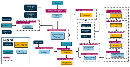
Figure 1. Proposed framework for Synthetic Population Generation and Agent-Based Transport Modeling, tailored for Brazil.

The framework implemented in Figure 1 is fully documented in Jupyter Notebooks with Python 3 codes available in the Supplementary Materials. Each described phase corresponds to one or more notebooks detailing the procedures for obtaining and processing data, statistical methods, model architecture, hyperparameter configuration, and validation. For instance, population synthesis procedures are documented and can be executed using notebooks 1.1_PopSimBR_dataWrangling.ipynb and 1.2_RunPopSimBR.ipynb. Activity scheduling models, found in notebooks 5.1.1 to 5.5, present complete specifications of model architectures, including activation functions, loss functions, layer configurations, and the training process. Sharing the codes not only enables reproducibility but, through the considerable documentation effort, helps researchers adapt the framework to other locations.

2.2.1. Population Synthesis

The framework starts with the creation of a synthetic population. A key source for the population synthesis is the Census Data [67]. The census data are divided into two: the universe and the sample. Due to time and budget constraints, microdata are available for a small sample of the population, usually between 5% and 20%, depending on the city’s total population, and have information about each household, dwelling, individual family member, and the weighting area they live in. The second is the universe, in which total figures of the population, used as controls for data fitting, are available in a more geographically coarse way, the census tract. Several methods for population synthesis exist and reviews of these methods can be found in [68,69,70]. In the context of Brazil, Ajauskas and Strambi conducted a comprehensive analysis of population synthesizers and introduced an extension called PopulationSimBR [71], specifically designed to address unique characteristics of Brazil’s data availability. PopulationSimBR, as an entropy maximization-based synthesizer derived from PopulationSim [72], which is an improvement from the work of Vovsha et al. [73], has functionalities such as the use of imperfect control totals, the optimized integerization of fractional expansion factors, and the use of controls at multiple geographic scales, both larger or smaller than the seed.

As a well-documented method, with a shared code, and tailored for Brazil, PopulationSimBR was selected for population synthesis. Modifications to the original code were the integration of a census data downloader using municipal codes and the incorporation of temporal adjustment of totals for population and household for any specified year within the 2010–2022 period. This last modification was considered essential given the temporal mismatch between available microdata (2010 census) and the more recent aggregate population and household totals available for the 2022 census tracts.

The temporal adjustment methodology uses scaling factors based on the ratio between population and household counts in 2022 and 2010 for each census tract, with interpolation applied to achieve estimates for intermediate target years. In this perspective, control totals are recalculated exclusively for these two demographic variables. Although this approach may introduce calibration challenges and assumes demographic stability in household composition over the adjustment period, it provides more accurate estimates in overall population numbers in years between the 2010–2022 timeframe.

The population synthesis procedure starts with the aggregation of control totals available at the census tract scale to the microdata scale of the weighting areas. Next, balancing, which redefines the weights provided by the census for each household, and integerization, which transforms the weights into integers, are applied. Both processes are constrained linear problems that are first repeated with the aggregate values for all census tracts then to the total of each census tract. This process results in the transformation of the household weights from the weighting area to the census tract.

2.2.2. Main Activities Allocation

The following phases of the framework involve the allocation of families to dwellings and of mandatory activities. The construction of the synthetic population included detailed information on residential structures to enable seamless integration with land use models. This information included the type of home, the status of the lease (owned or rented), the value of the lease, and the number of bedrooms and bathrooms. Using these attributes, along with the location of each dwelling at the census tract level, a matching procedure was implemented to define housing characteristics with records from the National Address Registry for Statistical Purposes (Cadastro Nacional de Endereços para Fins Estatísticos, CNEFE) [74]. CNEFE presents information on dwellings, establishments, and buildings under construction such as the name of the establishment and the type of dwelling (e.g., house, apartment, or gated community). Collected during the 2022 census fieldwork, it enables a more precise spatial allocation of synthetic families to a dwelling.

The framework then implements the creation and allocation of primary activities, a fundamental component that establishes educational and workplace locations for students and workers within the synthetic population. Determining these destinations for each person is critical for subsequent modeling steps, as the distances to these mandatory activities are key elements in estimating both the number and spatial distribution of daily activities.

The allocation of primary activities is based on the concept of a travel time budget [75,76,77,78]. Although the temporal stability of individual travel-time budgets is a subject of ongoing academic debate, this theoretical framework provides essential insights into behavioral constraints: individuals who spend substantial time commuting and executing mandatory activities (work, education) typically have reduced probability for participating in discretionary activity. Through explicit modeling of mandatory activity allocation, this framework generates the necessary spatial and temporal constraints to better represent the interplay between mandatory and discretionary activity patterns in subsequent modeling phases.

The construction of artificial workplaces used microdata from RAIS (Annual Social Information Report) [79] and the GeocodeBR 0.3.0 package [80]. The RAIS microdata comprises of two datasets: employment relationships and establishments. The employment relationship data set contains information on employees, including sex, age, educational level, municipality of employment, municipality of the home, establishment size, and occupational classification. The establishments data set, in turn, provides information such as the municipality of the establishment, the number of employment relationships by contract type, the classification of activity for the establishment, the legal status and the zip code.

Due to data protection laws, it is not possible to directly link individual employment records to specific establishments-such as with a common identifier between the two datasets. To address this limitation, a statistical matching procedure was developed to associate each employment record with an establishment, based on varying levels of matching precision. The process begins by comparing all available variables common to both datasets; this process creates a pool of possible choices that is selected probabilistically, weighted by the remaining number of available positions of the establishments. When the employment record is assigned to that establishment, the number of available positions is subtracted by one, reducing the probability of being selected. If no suitable establishment is identified with all possible variables, the matching criteria are progressively relaxed: first by omitting legal status, then establishment type, size, activity class, and neighborhood, until only the municipality remains as the matching criterion. Upon completion of the matching process, the resulting linked records are geolocated using the postal code information and the GeocodeBR package.

The allocation of educational establishments within the synthetic population framework was based on both the GeoBR 0.2.2 package [81] and microdata from the higher education census [82]. GeoBR, available in Python and R, streamlines the acquisition of geospatial data from a range of official Brazilian sources. Among the data sets are those related to schools and daycare centers, which include detailed attributes such as educational level, administrative category (public or private), institution size (as number of enrollment categories), and precise geographic coordinates (latitude and longitude). For higher education institutions, university addresses were georeferenced using the GeocodeBR package, allowing the identification of campus locations by latitude and longitude, as well as the corresponding enrollment figures for each campus.

With detailed individual characteristics available for the synthetic population, as well as datasets of artificial educational and workplace establishments, the assignment of primary activities was undertaken through a probabilistic matching process. Similarly to previous steps, this procedure builds identifies locations with similar attributes (person and establishment), filters possible matches, and probabilistically selects a place while dynamically reducing the likelihood of subsequent selections of this same place to ensure diversity.

For workers, the synthetic population includes information on the travel time to work, categorized into discrete intervals. Consequently, the allocation of workplaces uses demographic and occupational attributes such as age, education level, employment class, and municipality, but also applies a spatial filter to restrict potential workplaces to those within the travel time reported between home and place of work.

For students, the allocation of places of education uses a weighted selection probability based on empirical distributions obtained from Household Travel Surveys (HTS). After the filtration process of educational facilities by the person’s characteristics, such as the level of education in which it is enrolled, the selection probabilities are adjusted according to this distance distribution, working as a soft constraint to better approximate observed travel patterns. An important aspect in this process is the reporting of school enrollment figures in categorical ranges (up to 50 enrollments, 51–200, 201–500, 501–1000, 1000+). To assign selection probabilities proportional to enrollment size, the midpoint of each category was used as an initial weighting factor (25, 126, 351, 751, 1000).

2.2.3. Activities Scheduling

The fourth phase focuses on the creation of spatial variables linked to household locations and the standardization of data between the HTS and the synthetic population. In some instances, variables from the synthetic population were aggregated to match the categorical structure of the HTS, while in other cases, HTS variables were consolidated to correspond with the synthetic population’s classifications. In addition, travel purposes were grouped based on similarity and frequency within the data set.

Subsequently, both datasets were enriched with spatial variables. As previously mentioned, linear distances were calculated between households and allocated workplaces and educational institutions. In addition, spatial indicators were incorporated, including the number of households and commercial establishments in the vicinity of each residence, calculated by the 530-m-side hexagon [83] values the household falls in. Shannon’s entropy was derived from these two categories, and the distance from each household to the area with the highest concentration of establishments within the study area was also calculated. This last variable is a proxy of a common category usually implemented in models, that is, the class of the area the household dwelling is in-city center, urban area, fringes, rural areas, and so forth, which would need a priori determinations and assumptions.

Phase five represents the generation of individual activity plans within the synthetic population, resulting in the demand. In a limiting perspective, demand models may be divided into two: econometric and computational methods [84,85]. Econometric models, such as CEMDAP [86], are frameworks based on utility maximization, usually as linear functions of individual, environmental, and trip characteristics. These models have the advantage of allowing statistical testing and variable effects evaluation. However, they are often criticized for assuming utility maximization, inadequately representing flawed choices, having limited capacity to capture complex relationships, and requiring rigorously defined structures, interactions, and rules, which often necessitate significant expert input.

In contrast, computational models implements a series of rules and heuristics to establish relations between modeled attributes and activity patterns, as exemplified by ALBATROSS [87,88]. The specificity of these rules may vary from being predominantly predefined to being entirely defined by data, the latter commonly known as machine learning (ML) models. Data-driven methods, such as DDAS [89], offer several benefits relevant to the objectives of this study. By allowing algorithms to identify optimal input-output relations, these approaches eliminate the need for modelers to manually assess variable distributions, determine functional forms, or impose restrictive assumptions [90]. Furthermore, another relevant aspect of data-driven models is that, through the implementation of machine learning models, complex and nonlinear relationships are better captured and challenges related to model calibration in extensive databases are reduced. The latter is an increasingly common context in the field of transportation and land use modeling.

The use of machine learning also presents challenges. The complexity of hyperparameter tuning, the overfitting risks, the lack of transparency of models and interpretability of variable effects are just some of these. To effectively tackle some of these challenges, it is essential to consider dividing the data into training, testing, and validation sets. Furthermore, it is important to consider methods such as cross-validation and strategies to address sample imbalance in classification tasks. In terms of interpretability, recent advances have considerably reduced the problems associated with variable effects on model estimates, such as permutation feature importance [91] and SHAP [92].

In terms of effectively creating the activity plans, this study proposes a sequence of automated processes that, provided data standardization and enrichment are correctly performed in previous phases, the supplied scripts will set up the environment, preprocess the variables, partition the dataset, train and evaluate the model, apply the trained model to the synthetic population, and prepare the data for the subsequent step of the phase.

The first step involves training a classification model to determine whether an individual participates in travel-related activities. The second model estimates the number of out-of-home activities performed for individuals classified as engaging such activities. The classification methods evaluated were Random Forest [93], CHAID-induced decision tree [88], Support Vector Machine (SVM), Naive Bayes, Multi-layer Perceptron (MLP), Gradient-Boosted Trees and eXtreme Gradient Boosting Decision Trees (XGBoost) and the selection was based on test accuracy. XGBoost demonstrated the best performance.

XGBoost [94] is a gradient-boosted decision tree widely recognized for its high performance in both regression and classification tasks that involve structured data. Some of its advantages are scalability, robustness to outliers and noise, and integrated regularization mechanisms that mitigate overfitting. Another advantage of XGBoost is that it outputs prediction probabilities for classes, enabling stochastic classification modeling. This approach is consistent with empirical observations from the data, where individuals with identical profiles can exhibit heterogeneous activity patterns, as implemented in other frameworks [49,88,89].

The process activity durations assignment uses a probabilistic sampling approach based in empirical distributions of durations for pairs of activities, specifically the target activity and its predecessor. This method was implemented to account for the variability in duration patterns associated with the same activity, such as how the duration distribution for work activities varies based on whether the preceding activity was at home or meal. An acceptance control mechanism was incorporated into the sampling framework to maintain temporal consistency and adhere to realistic scheduling constraints. This control system assesses the activity durations by comparing the activity end times with the overall distribution of activity end times. When excessively long durations are allocated to early-sequence activities, the resulting end times are near the daily limit (e.g., 24 h), which restricts the possible duration range for later activities and may compromise the validity of the schedule. When no valid duration samples can be generated under these constraints, the sampling process is repeated.

The following steps employ Bidirectional Long Short-Term Memory (BiLSTM) networks [95] to model the activities to be performed, the locations where these activities will take place, and the transport mode for each individual. BiLSTM networks are recurrent neural networks that process input sequences in both forward and backward directions. Although the application of LSTM and BiLSTM networks for activity scheduling remains limited [96,97], these models are particularly well suited for problems characterized by sequential decision making, in which previous sequence states influence subsequent output. The inherit dependencies and feedback mechanism of the activity-scheduling problem naturally support the evaluation of such methods. Furthermore, key findings from Arkoudi et al. [96] demonstrate that direct use of static and dynamic variables as input to the LSTM layer outperforms approaches in which these variables are processed separately by a dense and a LSTM, respectively.

At the end of phase 5, the hourly departures for car and public transport trips are evaluated and compared to the observed distribution in the HTS. Visual and statistical analysis are performed to jointly assess the accuracy of durations, departure times, and mode choice for individuals in the synthetic population.

2.2.4. Agent-Based Simulation

Phase six involves executing the MATSim simulation, which includes all the procedures required to convert input data into files compatible with the software, as well as the evaluation of the simulation results. The initial process involves transforming the activity schedules to an XML format. For this purpose, the MATSim Python Tools library [98] was used. Each record was converted into individuals with specific attributes such as age, sex, household income, and educational level, in addition to the characteristics of activities and travel modes. In addition to plan generation, this official library provides a set of functionalities to facilitate the processing, analysis, and manipulation of data for MATSim within a Python environment, including network processing, event file manipulation, and calibration.

The construction of the public transport network required overcoming three primary challenges: (1) developing a historical network, (2) merging multiple General Transit Feed Specification (GTFS) datasets, and (3) integrating all processes within a unified computational environment. To build a historical network compatible with the year of the HTS and the available count data, the historical OpenStreetMap (OSM) file provided in the Geofabrik raw index directory was used [99].

The development of the multimodal transport network utilized two primary libraries: gtfs-kit [100] and pt2matsim [101]. The gtfs-kit library facilitated the integration of multiple public transport data sources, with the resulting data set later validated using the gtfs-validator [102]. For the construction of the multimodal network, pt2matsim was used to simplify the network and, with the integrated GTFS data, generate the integrated network, transit schedules and vehicle definitions required for public transport simulation in MATSim. Furthermore, the motorcycle mode was incorporated into all network links where car access is allowed.

Upon completion of the network creation, in addition to the XML files required by MATSim, geoparquet files containing node and link data are also exported to enable analysis of the generated network through commonly available GIS software, allowing multiple possibilities beyond the JOSM MATSim plugin [103]. Furthermore, this procedure was deemed essential to support multiple alternatives for associating available traffic count flows with the MATSim network link IDs, a manually performed task.

The files obtained are used in the MATSim agent simulation. In terms of changes that an agent can make in their original plans, as the framework already accounts for mode selection, activity durations, and destination changes, only the agent’s route choice is enabled. Thus, in the complete framework, MATSim receives the list of individual activity and travel plans and assigns them to the network. It should be noted that, as traffic assignment represents the most significant part of runtime, a commonly used workaround is scaling down the capacity of the network and sampling agents to produce similar outputs without the same complexity [104,105,106], a practice that is also used in this framework.

Model validation represents a critical component of agent-based modeling, though it presents substantial methodological challenges due to the complexities of agent’s simulation. The validation process, defined as the assessment of a model’s capacity to reproduce target system behavior, becomes particularly problematic when both the underlying system and the agent-based model exhibit complex, open-ended, and emergent-based characteristics [29]. From this perspective, some argue that an agent-based model demonstrating perfect similarity with observed data should be regarded with skepticism [107].

Three principal validation approaches for agent-based models can be distinguished. First, global validation (or fit-to-data validation) constitutes the most widely employed yet frequently criticized method, involving direct comparison between modeled outputs and real-world observational data. Second, face validation (or ontological structure examination) requires modelers to assess whether model behavior under specific modifications appears theoretically sound and empirically plausible. Third, pattern-oriented validation evaluates the correspondence between agent behavioral patterns on multiple spatial and temporal scales with empirically observed patterns. Among these approaches, pattern-oriented validation demonstrates the greatest potential for methodological advancement, particularly given the expanding integration of novel algorithmic techniques within agent-based modeling frameworks.

The validation of the framework was performed through a combination of the three approaches. The primary objective of this work is to introduce an open source framework that leverages publicly available datasets while minimizing predetermined structural and hierarchical constraints, thereby establishing a foundational platform for subsequent enhancements and adaptation within places with low data and technical availability. Given this foundational scope, validation criteria were deliberately calibrated to accommodate the objectives of the framework rather than to pursue exhaustive validation protocols.

An additional innovation implemented in this study involved the deployment of a unified computational environment through Google Colab. This approach eliminates the technical barriers associated with the configuration of diverse computational environments across heterogeneous machine architectures and operating systems, facilitating immediate code execution. Also, by adopting Colab’s, cross-platform compatibility by seamlessly integrating programs and libraries developed in alternative programming languages, including R-based GeocodeBR and Java-implemented MATSim is enabled. The development of an automated method for the installation, configuration, and execution of both PopulationSim and MATSim within these online notebooks further enhances the reproducibility and accessibility of the proposed framework.

3. Results

The framework was implemented in the Fortaleza Metropolitan Area (FMA), the sixth largest metropolitan area in Brazil, with a population of 3,903,924. The selection of FMA as the case study was based on four main criteria: (1) the population size of the region is sufficiently large to introduce modeling complexity, yet it does not constitute an outlier among Brazilian metropolitan areas; (2) the metropolitan public transport system is composed of multiple entities, including metro, train, municipal bus, and intermunicipal bus systems, each providing distinct data feeds, thus presenting a significant data integration opportunity; (3) the availability of municipal public datasets to check feasibility based on national information; and (4) the authors’ knowledge of the local context.

The first phase, of synthetic population creation, used 2010 and 2022 census data to achieve the number of households reported in 2018, the year of the HTS. The controls used in the process were (i) total households; (ii) households by family size (1, 2, 3, 4, 5, 6+); (iii) households by type (house, gated community, apartment); (iv) households by age of household head (≤29, 30–44, 45–59, ≥60); (v) households by per capita income class (less than 0.5, 0.5–1, 1–2, 2–3, 3–4, 4–5, ≥5 minimum wages); (vi) individuals by gender; and (vii) individuals by age group (under 4, 5–14, 15–19, 20–29, 30–39, 40–49, 50–59, 60+). The application of PopulationSimBR for 2010 resulted in errors below 1% for all variables except for the number of apartments (3.17%). To adjust the population in regions’ development between 2010 and 2022, scaling factors were applied to the control totals for households and individuals to reach the intermediate year of 2018, reference year for the FMA household travel survey.

As described in Section 2.2.1, although this update process introduces fitting errors and assumes a constant family composition, which is known to have changed, priority was given to obtaining household and population counts consistent with expected values from the HTS rather than to maintaining the accuracy of area-specific distributions. After adjustment, the household and population errors were 0.1% and 8.86%, respectively, which was deemed acceptable for a framework evaluation.

The following implementation phases encompass the generation of synthetic educational and employment establishments, the assignment of households to dwellings, and the allocation of workplaces and educational institutions to employed and enrolled individuals. As previously depicted, these assignments employ statistical matching procedures in which potential allocation pools, generated through individual characteristic profiles, are weighted according to empirically derived home-to-work and home-to-school travel distance distributions obtained from Household Travel Survey data collected during the Fortaleza Sustainable Accessibility Plan (PASFOR) [108].

The HTS was conducted in the 13 municipalities in the metropolitan area, from September 2018 to October 2019. The sampling was based on the total number of households derived from the electricity consumption data, which, after filtering for residential consumers, resulted in 1,231,030 records. Of these, 28,956 households were selected, of which 23,703 gave valid interviews, representing a sample of 1.92% of households. This sample was stratified by the average monthly energy consumption classes, a proxy of income, and a confidence level of 90% was ensured for all 317 traffic zones.

The allocation of households, workplaces, and educational institutions was validated by comparing observed distributions (obtained from the HTS) and those generated in phases 2 and 3 of the framework (synthetic). Figure 2 present the distance distributions between home and school and home and work, respectively. Regarding home-to-school distances, the Q-Q plot correlation coefficient was 0.95, indicating substantial similarity; however, the Kolmogorov-Smirnov test indicated that the distributions are statistically different. In terms of mean values, the average distance in the synthetic population was 3.82 km, compared to 2.92 km in the real population, which corresponds to a relative error of approximately 31%. Quartile analysis revealed that the synthetic population exhibited a first quartile of 1 km compared to 440 m in the observed population, indicating a bias toward longer distances in the educational synthetic allocation process, which may affect shorter-distance travel patterns that characterize substantial portions of educational trip-making behavior.

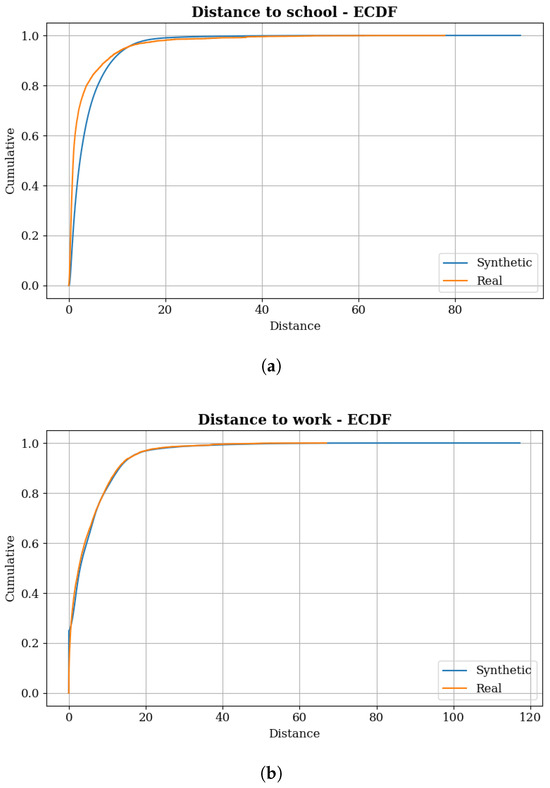
Figure 2. Observed and Synthetic Empirical Cumulative Distribution Function of Distance: (a) Distance to school. (b) Distance to work.

One factor contributing to this greater divergence in distances may be related to the assumption adopted for the probability of selecting educational institutions. Using the midpoint of the available enrollment classes as the actual number of possible enrollments for a school, the real capacity of many educational facilities have been significantly underestimated. This is particularly true for the highest class, schools with more than 1000 enrollments, for which a capacity of 1000 was assigned. This potential enrollment bottleneck may have resulted in a pool of possible allocations smaller than reality, leading to longer travel distances.

With respect to home-to-work distances, the distributions are more similar (Figure 2), with the largest difference observed in the tail. The Q-Q plot correlation coefficient was 0.99, even higher than for home-to-school distances, and the differences in mean, median and quartiles were minimal: the mean was 5.32 km for the synthetic population and 5.08 km for the real population, a relative error of 4.63%; the median was 2.86 km for the synthetic population and 2.6 km for the real population. Despite this greater similarity, the results of the Kolmogorov-Smirnov test indicated that the distributions are statistically different. Table 1 presents the results for the distance to school and distance to work values.

Table 1. Summary table of main activities allocation.

Metric	Observed (HTS)	Synthetic	Absolute Difference	Relative Error (%)	Statistical Test
Home-to-School Distance
Mean (km)	2.92	3.82	0.9	30.82
Median (km)	0.91	2.34	1.43	157.14	KS: p > 0.001
Q1 (km)	0.44	1.00	0.56	127.27
Q-Q Correlation	–	0.95	–	–
Home-to-Work Distance
Mean (km)	5.08	5.32	0.24	4.72
Median (km)	2.60	2.86	0.26	10.00	KS: p > 0.001
Q1 (km)	0.47	0.06	−469.94	−99.99
Q-Q Correlation	–	0.99	–	–

A notably distinct element is the maximum value, given the long tail of the synthetic population distribution. Although the maximum value in the real population was 67 km, in the synthetic population it was 117 km. We believe that a relevant factor contributing to this difference is the employment data, which does not account for informal employment, potentially exacerbating the spatial mismatch between workers and workplaces. In fact, recent studies, including those focused on Fortaleza [109], have demonstrated that incorporating data on informal employment reduces these inequality issues and, therefore, could decrease the maximum distances from work by creating a more dispersed concentration of working places. However, the absence of more spatially disaggregated information makes such an analysis unfeasible.

In phase 4, which involved the standardization of columns in both training input (HTS) and synthetic data, trip purposes were consolidated and activity chains with a frequency lower than 20 were excluded to prevent significant class imbalance. The grouping was defined as follows: ‘Accompany someone for health’: ‘A’; ‘Accompany someone for study’: ‘A’; ‘Accompany someone for work’: ‘A’; ‘Accompany someone for other reasons’: ‘A’; ‘Personal matters’: ‘O’; ‘Shopping’: ‘B’; ‘Study (other courses)’: ‘S’; ‘Study (regular)’: ‘S’; ‘Leisure’: ‘L’; ‘Doctor/Dentist/Health’: ‘M’; ‘Other’: ‘O’; ‘Job search’: ‘O’; ‘Meal’: ‘R’; ‘Home’: ‘H’; ‘Work’: ‘W’; ‘No purpose’: ‘NoTrip’.

In the activity scheduling phase, which involved training the steps to predict the activity plans of each individual in the synthetic population, the data set was split into 70% for training and testing and 30% for validation. In the first step, which consists of the sequential prediction of whether an individual engages in out-of-home activities and, subsequently, the number of activities performed, XGBoost algorithms were used for binary and multiclass classification, respectively.

Hyperparameter optimization was performed with Optuna [110], a Bayesian optimizer, to determine the optimal hyperparameters that maximize the area under the ROC curve. The search space included the following hyperparameters: number of estimators, maximum tree depth, learning rate, subsample ratio, minimum loss reduction, L1 regularization term, and L2 regularization term. The optimization process was limited to a maximum of 1000 trials or 4 h and a stratified K-fold cross-validation was implemented to mitigate the risk of overfitting. Class weights calculated based on sample frequency were applied in the multiclass problem to address class imbalance.

For the binary case, the model with optimized hyperparameters achieved a ROC AUC of approximately 0.86, indicating strong predictive performance. In the validation set, individual-level predictive accuracy was 80.26%. The comparison of actual and predicted distributions presented an even closer alignment, with the difference between actual and predicted counts being less than 0.5%.

In the multiclass, the model with optimized hyperparameters yielded a one-vs-rest ROC AUC of 0.79, also indicating good predictive performance. Although the overall accuracy of 85.25%, analysis of the confusion matrix revealed a predominance of predictions for two out-of-home activities, reflecting the unbalanced distribution of the data set even though sample weights were applied. Among the errors, adjacent classes (classes 2, 3, and 4) misclassification was predominant and the most distant class, corresponding to six out-of-home activities, was not correctly predicted in any case. When evaluating the overall distribution, the absolute errors increased as the distance from two activities increased, although the class proportions were quite similar, with the largest difference being −1.4% for four activities.

During the activity determination stage, the model input is divided into two distinct types: static and dynamic input. Static input variables are those that do not vary across the steps of the activity chains and are related to sociodemographic, household, and dwelling characteristics. These static attributes include: age, gender, car availability, motorcycle availability, educational enrollment, family relationship, main activity status, distance to workplace, distance to educational institution, number of establishments in the vicinity of the dwelling, number of dwellings in the vicinity of the dwelling, entropy calculated by the number of establishments and dwellings in the vicinity, distance to the hexagon with the highest number of jobs, family size, and the number of out-of-home activities previously assigned to each individual.

The dynamic input, which changes at each step, was defined as the step index, representing the position in the sequence from one up to the maximum of activities performed in the population, which was six. An additional preprocessing step was applied to the dynamic input, in which the positions corresponding to activities beyond the number defined in the previous stage were assigned a value of zero.

With respect to model architecture and optimization, the dynamic input is first processed by an Embedding Layer, which converts each step index into a vector representation. During this process, zero values are masked to ensure that padding does not influence the model’s learning. Following the approach recommended in Arkoudi et al. [96], the static and dynamic inputs are combined and then processed by a BiLSTM layer, followed by a TimeDistributed layer with a softmax activation function to generate model predictions.

For the neural networks, hyperparameter optimization was performed using the hyperband algorithm implemented via the KerasTuner library [111]. The search space included embedding dimension (8, 16, 32, 128, 256), dropout rate (0.0, 0.1, 0.3, 0.5), recurrent dropout rate (0.0, 0.1, 0.3, 0.5), number of units (ranging from 32 to 512 in increments of 32), and learning rate (from $1\times {10}^{-4}$ to $1\times {10}^{-2}$, using log-uniform sampling). The class imbalance was addressed by applying class weights calculated based on the frequency of activities.

The optimization process used an early stopping criterion based on a minimum improvement delta of 0.0001 in sparse categorical precision and a patience parameter of five epochs. The optimal hyperparameters were: embedding dimension of 32, dropout rate of 0.1, recurrent dropout rate of 0.5, and 352 LSTM units. Under these hyperparameters, the best-performing model achieved an accuracy of approximately 0.94, indicating a high level of predictive performance.

Regarding the distributional analysis, the chi-square test indicates that the observed and predicted distributions in the validation set are not similar as the test statistic approached infinity, primarily due to the generation of travel chains that do not exist in the empirical data, an expected and desirable outcome. The BiLSTM predicts one activity at a time to create the complete chain of activities, an open-ended chain determination model. This approach enables the emergence of novel activity sequences not represented in the original training set, extending the model’s capability beyond the empirically observed patterns.

The high predictive accuracy and the minimal differences observed among the most frequent activity chains (see Figure 3) indicate that the model performance is satisfactory for practical purposes. Furthermore, the distributional error appears to be primarily associated with specific classes misclassifications (e.g., reassignment of activity decisions from chains such as H-O-H to H-M-H). This suggests that the error is not indicative of a substantial shift in the overall population activity chain distribution, such as the dominance of one or more chains, but rather reflects misclassification among particular discretionary activity.

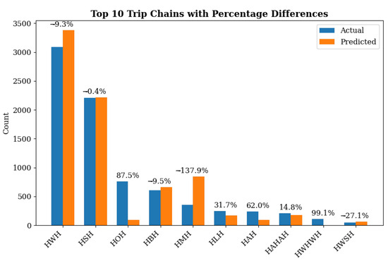
Figure 3. Distribution of Activities Chains in Validation vs. Predicted Data.

The durations and end times of the activities were determined by probabilistic sampling from empirical distributions derived from the observed activity dataset. This data-driven methodology exhibited strong similarity to empirical patterns, as the sampling procedure draws directly from observed behavioral data to populate the synthetic population (see Figure 4 for distributional comparisons and Table 2).

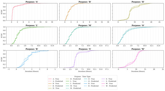
Figure 4. Activities Duration Distributions in Validation vs. Predicted Data.

Table 2. Mean Absolute Error of activities durations.

Activity	Mean Absolute Error
A–Accompany	74.47 min
B–Shopping	74.82 min
H–Home	183.97 min
L–Leisure	109.26 min
M–Health	107.43 min
O–Others	140.63 min
R–Meal	44.67 min
S–Study	95.72 min
W–Work	165.31 min

However, this approach presents a significant methodological limitation: the absence of correlation between assigned temporal parameters and individual-level characteristics. Specifically, the duration assignment process operates independently of participants’ sociodemographic attributes and spatial variables, thereby failing to capture the heterogeneity in activity patterns that may be attributable to these demographic and geographic factors. This limitation constrains the model’s capacity to represent the differential temporal behaviors exhibited across population subgroups.

As in the activity determination stage, the determination of activity distances and locations utilizes both static and dynamic input. For static input, the same variables used previously were used. Regarding dynamic input, in addition to the position of the sequence, the activity sequence and the end time of each activity were also included. A custom masked mean squared error loss function was implemented to exclude masked steps from the loss calculation. Similarly, a custom mean absolute error metric was used, also configured to ignore masked steps. In terms of architecture, the optimized model resulted in two BiLSTM layers with 256 units and a dropout rate of 0.1. The model achieved a mean absolute error (MAE) of approximately 1.5 km.

Following the prediction of activity distances, location imputation was performed using establishment data from the CNEFE database. In an iterative process, the destination location for each activity was determined through a spatial filter defined by a ring with boundaries set to the predicted distance plus or minus a step size, initially established as 10% of MAE. If no suitable location was identified within this range, the step size was incrementally increased until at least one eligible location was found.

In terms of transport mode prediction, information on the travel distances derived from the last step and characteristics related to travel times and costs for each mode (walking, bicycle, public transport, car and motorcycle) was added to the dynamic input for each leg of the individual’s journeys based on their origin and destination zones. Furthermore, transport modes were mapped as follows: ‘Shuttle bus/Jitney’, ‘School bus’, ‘Metropolitan bus’, ‘Municipal bus’, ‘Executive bus’, and ‘Subway/Light rail’ were grouped under ‘pt’ (public transport). ‘Own bicycle’ and ‘Shared public bicycle’ were categorized as ‘bike’, ‘On foot’ to ‘walk’, ‘Car driver’ to ‘car’ while ‘Car passenger’, ‘Chartered transport’, ‘Taxi’, ‘App-based rides’, ‘Motorcycle passenger’ and ‘Motorcycle taxi’ were grouped as ‘ride’, ‘Motorcycle driver’ was classified as ’motorcycle’ and entries such as ’Others’, ’Truck’ and ’Urban freight vehicle’ were deleted.

The optimized model architecture comprises three BiLSTM layers with 256 units each, with a dropout rate of 0.3 applied only to the first two layers. A custom loss function and a custom masked accuracy metric were implemented to compute the weighted masked scores. The model achieved an accuracy of 0.64. Analysis of the distribution of predicted mode share (see Figure 5 and Table 3) indicates consistency between true and predicted values of the validation set, with a slightly higher representation of bicycle, motorcycle and car trips, and a lower representation for walking, public transport and rides.

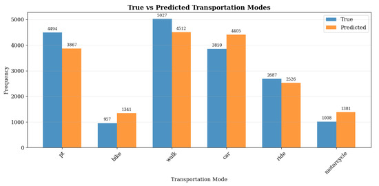
Figure 5. Mode Distribution in Validation vs. Predicted Data.

Table 3. Summary of Mode Distribution in Validation vs. Predicted Metrics.

Mode	Validation	Predicted	Absolute Difference	Relative Error (%)
Public Transit	4494	3867	−627	−13.95
Bike	957	1341	384	40.13
Walk	5027	4512	−515	−10.24
Car	3859	4405	546	14.15
Ride	2687	2526	−161	−5.99
Motorcycle	1008	1381	373	37.00

As described in Section 2.2, the activity scheduling process was carried out at each stage through training, testing, and validation of the models using the HTS dataset, followed by the prediction of these values for individuals in the synthetic population. In the mode choice stage, the modal split behavior differed considerably from the observed and synthetic behavior. Figure 6 compares the modal split between HTS and synthetic data, indicating that the share of bicycle and, especially, public transport modes is overestimated, while walking and car trips are underestimated.

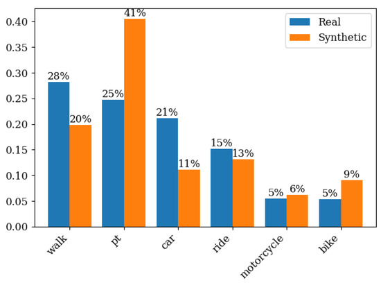
Figure 6. Mode Distribution in Synthetic and Real Data.

It is well established that prediction errors from earlier stages propagate throughout the sequence, thereby decreasing the predictive accuracy of subsequent phases; consequently, models applied later in the sequence are affected by the errors of the preceding ones [112]. The errors observed in transport mode prediction exemplify this cumulative effect, with the synthetic population generation acting as a key contributor driving the discrepancies. The synthetic population generation process relies exclusively on census data, without incorporating controls derived from the Household Travel Survey, resulting in family compositions that reflect 2010 census characteristics with substantially lower motorization levels. This methodological choice may contribute to systematic underestimation of cars trips within the model framework.

The exclusion of HTS data from the population synthesis process was implemented to reduce complexity in multiple data sourcing and wrangling, since population synthesis represents one of the most resource-intensive components in the development of disaggregated models. Brazilian HTS datasets exhibit municipality-specific variations and considerable heterogeneity in data transparency, availability, and methodological approaches, necessitating extensive data mapping and integration procedures for incorporation into PopulationSimBR. As a solvable framework drawback in the future, due to updated distributions from the 2022 Census becoming available and being used as controls, this limitation is not considered critical for future implementations.

Empirical evidence supporting this assessment emerges from comparative analysis of vehicle ownership patterns between the 2010 census and 2018 HTS data. While motorcycle availability remained relatively stable (13.17% to 16.17%), household car ownership increased substantially from 23.97% to 45.67%, representing a near doubling of car ownership rates. This difference underscores the temporal mismatch between census-based population synthesis and HTS travel behavior patterns. These methodological limitations and potential solutions are examined in a comprehensive way in Section 4.

Analysis of hourly trip distribution patterns by transport mode in Phase 5 reveals differences between observed data, derived from HTS trip expansion factors, and synthetic model outputs. The synthetic population systematically underestimates car trips while significantly overestimating the use of public transport relative to empirical observations (see Figure 7).

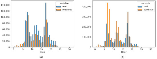
Figure 7. Observed and Synthetic Sum of Hourly Trips: (a) Car. (b) Public Transit.

In terms of the multimodal transportation network, it was constructed using road network data from January 2019, sourced from the Geofabrik database [99]. The data set was geographically delimited to the Fortaleza metropolitan area and was pre-processed by removing unconnected nodes and isolated subgraphs. GTFS data for metro, train and light rail transit (LRT) systems [113], municipal bus services [114], and inter-municipal bus services [115] were integrated. As a result, the multimodal network topology, transit schedules, and vehicle data sets were generated.

Due to the absence of comprehensive databases containing information on routes, stops, frequencies, and vehicles, the municipal bus networks of municipalities other than Fortaleza were not implemented. Consequently, the access to public transportation in these municipalities is represented solely by the inter-municipal network. Furthermore, as indicated by the data sources, the available GTFS feeds correspond to more recent years than 2018. This anachronism may result in variations in public transport routes and travel times. However, given that the experiment is limited to rerouting, with no possibility of mode change, it was decided to maintain the networks, acknowledging that PT trip counts and travel times may be slightly affected.

The traffic counts data obtained from PASFOR surveys [108] are categorized into cars, motorcycles, and various types of trucks and buses. Temporally, the data are segmented into 15-min intervals, with counts available from 06:00 to 09:00, 10:30 to 13:00, and 16:30 to 20:00. To ensure compatibility with hourly data, the 15-minute intervals were aggregated into hourly periods. Trucks were excluded from the counts and all types of buses were assigned to the standard bus category. In the simulation, the same passenger car equivalent (PCE) values used in the accessibility plan traffic simulation were adopted: 1 for cars, 0.35 for motorcycles, and 2 for buses.

The trip allocation process in MATSim was conducted using a 10% sample of the population (approximately 270,000 agents). The QSim controller was employed, with a FIFO link dynamics approach and the network capacity was reduced to the same 10%. Public transport was simulated deterministically, based on the schedule developed during the multimodal network construction stage, and individuals could access the system by walking. The replanning strategy involved rerouting 40% of the population in each iteration, while the remaining 60% selected previously executed plans. A total of 200 iterations were performed. Walking, cycling, and ride-sharing modes were simulated as teleported.

4. Discussion

Consistent with the modal split and the hourly travel distribution discussed previously, the model systematically underestimated traffic flows relative to the observed count data (Figure 8). This trend is primarily attributed to the number of cars and motorcycles as the main element that governs the PCE flows on the network. The high number of individuals assigned to public transport does not generate new buses in the simulation, given the deterministic nature attributed to public transport in the configuration. Consequently, the effect of increased public transport demand is reflected in substantially lower simulation scores for users of buses, trains, metro, and light rail, as capacity constraints prevent many from boarding and executing their activities. The mean absolute error for all hours and types of roads was 422.92 and for the morning peak was 300.63. Although these error levels are high for operational planning purposes, they are deemed acceptable within the strategic and complex context of the simulation, especially in scenarios assessment use cases.

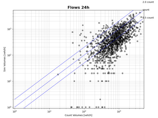
Figure 8. Counted vs. Simulated Traffic Flows for Each Hour.

A comparative assessment was also conducted against established Brazilian modeling practices. Figure 9 presents traffic assignment results from the proposed methodology (left panel) and the conventional four-step trip-based model implemented in PASFOR [108]. The peak-hour focus inherent in traditional models restricts comparative analysis to the morning peak period. Furthermore, differences in network topologies, link representations, and construction methodologies (e.g., unidirectional versus bidirectional link configurations) make direct flow comparisons unfeasible, restricting the analysis to visual inspection.

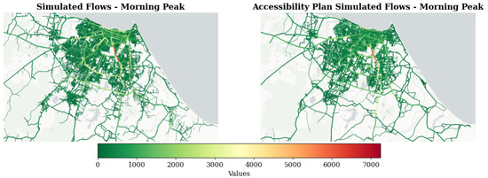
Figure 9. Comparison of Morning Peak Simulated Traffic Flows from Proposed Framework and Fortaleza’s Accessibility Plan.

Within these analytical constraints, both simulation approaches exhibit comparable spatial patterns during the examined period, demonstrating the framework’s potential applicability in practical planning contexts beyond academic research, subject to the limitations previously identified.

Furthermore, much of the models limitations are related to the anachronism of the input. The limited availability of data from the most recent census, which is being gradually released, required the construction of a synthetic population with household and family characteristics that corresponded to those of the last census with available microdata. As a result, the synthesized families are, on average, larger, younger, and less motorized. When combined with behavior modeled from a population nearly a decade later, the characteristics of trips, especially the choice of mode of transportation, diverged systematically. Another temporally affected element is the multimodal network. Although this limitation is mitigated by obtaining the HTS year road network from OSM, which solves the problem of traffic count validation in a network of the same year, the GTFS data used do not correspond to the modeled year.

Employment modeling presents additional limitations. Primary data sources provide information on formal employment, spatially referenced by postal codes. In cities such as Fortaleza, postal codes offer sufficient spatial granularity for disaggregated modeling, however, in smaller, less affluent cities, postal codes may represent the entire city, resulting in an unrealistic concentration of employment opportunities. Furthermore, the lack of consideration for informal employment is another important limiting factor, as accounting for job informality may reduce spatial mismatch and potentially decrease differences in simulated and observed travel distances. It is important to note that the omission of these aspects is due to the lack of specific information and partial identification of the mechanisms driving these phenomena, not a lack of recognition of their importance in shaping urban system dynamics.

The framework demonstrates the generalization, modularity and adaptability required for application in diverse Brazilian cities and metropolitan regions. Given that most of the input data used is available at the national level and minor data standardization at the city level is necessary, replication, further development, and enhancement of the framework modules are facilitated. Regarding computational feasibility, the cost of using high-performance machines through Google Colab is approximately 58 BRL, representing less than 2% of the average monthly income of Brazilian workers. It is also expected that the implementation of these studies will be carried out by public and private entities with greater financial capacity than the average worker, therefore, while a financial barrier exists, it is not considered prohibitive.

Future Work

Although the framework proposed in this study is capable of generating complex simulations that closely approximate observed urban mobility patterns, several opportunities for future research remain. The assignment of primary activity locations, especially those related to education, could be improved to better reflect empirically observed patterns of shorter trip distances. The current implementation, which relies on preexisting data libraries, does not account for several characteristics of educational establishments.

Regarding population synthesis, although most limitations will be addressed through future Census data releases, an alternative approach to updating synthetic population parameters involves incorporating data from the National Household Sample Survey (PNAD) [116], which maintains the adopted premise of a nationally available data usage. This survey provides annual microdata on vehicle ownership, motorcycle ownership, household income, age demographics, and other relevant variables, though at a coarser geographic resolution than Census data, such as the municipal level.

In terms of the scope and statistical reliability of the validation. Although the validation used multiple complementary approaches, such as distributional comparisons across behavioral dimensions, statistical hypothesis testing, traffic assignment validation at 168 locations, and temporal pattern analysis, all pertain to the same geographic and temporal context. This limitation hinders the claims of stability and generalization in different urban contexts, temporal conditions, and environmental factors. In this perspective, future work should extend validation by applying the framework to metropolitan areas with markedly different characteristics and by using household travel surveys from multiple years within the same city to test its ability to reproduce behavioral change over time. Such efforts will likely require coordinated, multi-institutional collaboration and shared resources. By providing a fully documented open source framework, this study aims to enable this type of collaboration. It is noteworthy that the present validation shows performance comparable to traditional models under realistic, data-constrained conditions, offering preliminary evidence of feasibility while underscoring the need for broader tests to establish robustness.

With respect to behavioral modeling, future research directions can be categorized into structural and methodological improvements. In terms of structure, the work by Koushik et al. [97] employs a time series modeling approach that simultaneously defines activities, durations, and departure times, thereby reducing the need for predefined structures and relationships, potentially minimizing cumulative errors. This approach could be further extended to jointly determine transport mode by creating new categories for trip class. Furthermore, the current framework does not include specific sociocultural factors that could affect travel behavior, including religious affiliation and cultural practices. This omission is due to limitations in data availability rather than theoretical factors, as most household travel surveys in the Brazilian context do not contain such variables. Future implementations in contexts where personal religion affiliation is collected and detailed travel surveys recognize religious or cultural activities as separate trip purposes should investigate these aspects of behavioral diversity.

From a methodological perspective, two main aspects stand out. First, the development of more comprehensive frameworks, with the integration of long-term decisions, such as land use changes, shifts in economic activities, and demographic changes (e.g., increasing education levels and population aging), is essential for evaluating the long-term impacts of interventions and policies. Currently, the framework addresses only medium-term decisions, focusing on mobility patterns and short-term behavioral responses. By explicitly modeling the effects of accessibility on urban density, employment generation, and other long-term decisions, as well as their reciprocal effects, future iterations of the framework could enable more robust analyses.

Second, current implementation assigns each employed individual to a single primary workplace, which simplifies the spatial allocation problem but does not explicitly represent individuals with multiple job locations. These simplifications maintain computational tractability and reflect the structure of available census data, which reports information about main job location only. Future extensions could incorporate multiple anchors for employed individuals by analyzing sequences of work activities in household travel surveys and estimating the probability of secondary workplace locations conditional on primary workplace characteristics and individual attributes.

Lastly, although the framework is designed to generate a final activity schedule for a MATSim simulation, considering an initial plan generator for further calibration is feasible and may present an opportunity for better validation. In this regard, MATSim extensions, such as Cadytis [117,118] may be adopted as a subsequent stage to calibrate the coefficients, thus improving the similarity of the simulated and observed count data.

5. Conclusions

Agent-based models are expected to play a critical role in urban planning and project evaluation in the coming decades. Whether due to policy sensitivity, better explaining urban processes, making applications more reliable, or minimizing urban planner communication barriers, Brazil, and other countries in the global south, should dedicate much of their efforts to developing agent-based models tailored for their complexities and heterogeneity.

This study contributes to the field by presenting an optimal generalizable approach for constructing synthetic populations, activity plans, integrated multimodal network, and agent-based simulations tailored to context and data environment similar with Brazil. The proposed methodology serves as a reference for future research, policy formulation, and practical applications.

Methodological advances are introduced by integrating data-driven techniques for activity modeling, reducing predefined decision structures, hierarchies, and need of expert knowledge. The modularity, flexibility, transparency, and reproducibility provided by the framework, along with the public availability of its source code, addresses critical limitations in the development of agent-based models, such as the lack of reproducible studies and the uneven distribution of implemented ABMs. It also enables a more policy-sensitive and population-heterogeneous alternative to traditional models, which are often excessively aggregated and top-down approaches. The validity of the framework is demonstrated through its application to the metropolitan area of Fortaleza, resulting in pattern-validated phases and a traffic assignment with a mean absolute error of 422.92, acceptable for strategic applications given the complexity of the context.

Identified errors are traced to specific components of the framework, such as data anachronism, which may be addressed in future work. Thus, despite certain areas for improvement, the framework demonstrates robustness and applicability, even with data limitations and contextual challenges.

A key advantage of the proposed approach is its reliance on nationally available datasets, which minimizes city-specific data standardization requirements and facilitates framework replication and enhancement. This design choice substantially reduces implementation complexity while maintaining analytical rigor, thereby providing a scalable and cost-effective solution to advance transportation modeling capabilities at the municipal level. The validation of the framework demonstrates significant potential for nationwide implementation and establishes a foundation for a broader adoption of agent-based modeling methodologies within Brazilian urban planning practice. Given the availability of travel data collection on a national scale, this approach enables the development of agent-based models for any Brazilian municipality, regardless of the limitations of the local data infrastructure. Consequently, these research findings contribute to national policy and academic debate on optimal pathways for implementing municipal-level agent-based models, thus bridging the gap between advanced analytical techniques and practical urban planning applications across a diverse socioeconomic landscape.

References

- Batty, M. Building a Science of Cities. Cities 2012, 29, S9–S16. [Google Scholar] [CrossRef]
- Ding, R. The Complex Network Theory-Based Urban Land-Use and Transport Interaction Studies. Complexity 2019, 2019, 4180890. [Google Scholar] [CrossRef]
- González, m.C.; Hidalgo, C.A.; Barabási, A.L. Understanding Individual Human Mobility Patterns. Nature 2008, 453, 779–782. [Google Scholar] [CrossRef]
- Song, C.; Koren, T.; Wang, P.; Barabási, A.L. Modelling the Scaling Properties of Human Mobility. Nat. Phys. 2010, 6, 818–823. [Google Scholar] [CrossRef]
- Bastarianto, F.F.; Hancock, T.O.; Choudhury, C.F.; Manley, E. Agent-Based Models in Urban Transportation: Review, Challenges, and Opportunities. Eur. Transp. Res. Rev. 2023, 15, 19. [Google Scholar] [CrossRef]
- Banister, D. The Sustainable Mobility Paradigm. Transp. Policy 2008, 15, 73–80. [Google Scholar] [CrossRef]
- Hickman, R.; Hall, P.; Banister, D. Planning More for Sustainable Mobility. J. Transp. Geogr. 2013, 33, 210–219. [Google Scholar] [CrossRef]
- Saujot, M.; de Lapparent, M.; Arnaud, E.; Prados, E. Making Land Use–Transport Models Operational Tools for Planning: From a Top-down to an End-User Approach. Transp. Policy 2016, 49, 20–29. [Google Scholar] [CrossRef]
- Banister, D. Unsustainable Transport: City Transport in the New Century, 1st ed.; Routledge: London, UK; New York, NY, USA, 2005. [Google Scholar]
- Vasconcellos, E.A. Transporte Urbano nos Paises em Desenvolvimento: Reflexoes e Propostas; Annablume: São Paulo, Brazil, 2001. [Google Scholar]
- Walks, A. Driving the Poor into Debt? Automobile Loans, Transport Disadvantage, and Automobile Dependence. Transp. Policy 2018, 65, 137–149. [Google Scholar] [CrossRef]
- Pero, V.; Stefanelli, V. A questão da mobilidade urbana nas metrópoles brasileiras (The evolution of commuting time in metropolitan Brazil between 1992 and 2013). Rev. Econ. Contemp. 2015, 19, 366–402. [Google Scholar] [CrossRef]
- Pereira, R.H.M.; Banister, D.; Schwanen, T.; Wessel, N. Distributional Effects of Transport Policies on Inequalities in Access to Opportunities in Rio de Janeiro. J. Transp. Land Use 2019, 12, 741–764. [Google Scholar] [CrossRef]
- maranhão, I.G.d.O.; Filho, R.D.O.; dos Santos, E.M. The Governmental Perspective in the Urban Mobility Plan-Making: The Case of Peripheral Municipalities of the Rio de Janeiro Metropolitan Area. Rev. Prod. Desenvolv. 2017, 3, 117–135. [Google Scholar] [CrossRef]
- Brazil. Law No. 10.257, July 10, 2001. Statute of the City. In Diário Oficial da União; Federal Government of Brazil: Brasília, DF, Brazil, 2001. Available online: http://www.planalto.gov.br/ccivil_03/leis/leis_2001/l10257.htm (accessed on 7 April 2025).
- Brazil. Constitutional Amendment No. 90, June 15, 2015. In Diário Oficial da União; Federal Government of Brazil: Brasília, DF, Brazil, 2015. Available online: http://www.planalto.gov.br/ccivil_03/constituicao/emendas/emc/emc90.htm (accessed on 4 April 2025).
- Brazil. Law No. 12.587, January 3, 2012. National Urban Mobility Policy (Política Nacional de Mobilidade Urbana). In Diário Oficial da União; Federal Government of Brazil: Brasília, DF, Brazil, 2012. Available online: http://www.planalto.gov.br/ccivil_03/_ato2011-2014/2012/lei/l12587.htm (accessed on 5 April 2025).
- Brazil. Law No. 13.089, January 12, 2015. Statute of the Metropolis (Estatuto da Metrópole). In Diário Oficial da União; Federal Government of Brazil: Brasília, DF, Brazil, 2015. Available online: http://www.planalto.gov.br/ccivil_03/_ato2015-2018/2015/lei/l13089.htm (accessed on 7 April 2025).
- Huang, J.; Cui, Y.; Zhang, L.; Tong, W.; Shi, Y.; Liu, Z. An Overview of Agent-Based Models for Transport Simulation and Analysis. J. Adv. Transp. 2022, 2022, 1–17. [Google Scholar] [CrossRef]
- Moeckel, R.; Llorca Garcia, C.; Moreno Chou, A.T.; Okrah, M.B. Trends in Integrated Land Use/Transport Modeling: An Evaluation of the State of the Art. J. Transp. Land Use 2018, 11, 463–476. [Google Scholar] [CrossRef]
- von Thünen, J.H. Isolated State an English Edition of der Isolierte Staat; Pergamon Press: Oxford, UK; New York, NY, USA, 1826/1966. [Google Scholar]
- Timmermans, H. The Saga of Integrated Land Use-Transport Modeling: How Many More Dreams Before We Wake Up? In Proceedings of the Conference Keynote Paper, Lucerne, Switzerland, 10 August 2003; p. 35. [Google Scholar]
- Chang, J.S. Models of the Relationship between Transport and Land-use: A Review. Transp. Rev. 2006, 26, 325–350. [Google Scholar] [CrossRef]
- Crooks, A.; Castle, C.; Batty, M. Key Challenges in Agent-Based Modelling for Geo-Spatial Simulation. Comput. Environ. Urban Syst. 2008, 32, 417–430. [Google Scholar] [CrossRef]
- Wee, B.V. Toward a New Generation of Land Use Transport Interaction Models: A Viewpoint. J. Transp. Land Use 2015, 8, 1–10. [Google Scholar] [CrossRef]
- Kii, M.; Nakanishi, H.; Nakamura, K.; Doi, K. Transportation and Spatial Development: An Overview and a Future Direction. Transp. Policy 2016, 49, 148–158. [Google Scholar] [CrossRef]
- Thomas, I.; Jones, J.; Caruso, G.; Gerber, P. City Delineation in European Applications of LUTI Models: Review and Tests. Transp. Rev. 2018, 38, 6–32. [Google Scholar] [CrossRef]
- Kii, M.; Moeckel, R.; Thill, J.C. Land Use, Transport, and Environment Interactions: WCTR 2016 Contributions and Future Research Directions. Comput. Environ. Urban Syst. 2019, 77, 101335. [Google Scholar] [CrossRef]
- Heppenstall, A.; Crooks, A.; Malleson, N.; Manley, E.; Ge, J.; Batty, M. Future Developments in Geographical Agent-Based Models: Challenges and Opportunities. Geogr. Anal. 2021, 53, 76–91. [Google Scholar] [CrossRef] [PubMed]
- Lopes, A.S.; Cavalcante, C.B.; Vale, D.S.; Loureiro, C.F.G. Convergence of Planning Practices towards LUT Integration: Seeking Evidences in a Developing Country. Land Use Policy 2020, 99, 104842. [Google Scholar] [CrossRef]
- Lowry, I.S. A Model of Metropolis; Technical Report RM-4035-RC; RAND Corporation: Santa Monica, CA, USA, 1964. [Google Scholar]
- Wegener, M. Overview of Land Use Transport Models. In Handbook of Transport Geography and Spatial Systems; Hensher, D.A., Button, K.J., Haynes, K.E., Stopher, P.R., Eds.; Emerald Group Publishing Limited: Bingley, UK, 2004; Volume 5, Chapter 6; pp. 127–146. [Google Scholar] [CrossRef]
- Mackett, R.L. Leeds Integrated Land-use Transport Model (LILT). Suppl. Rep. 1983. Available online: https://trid.trb.org/View/203733 (accessed on 20 January 2021).
- Putman, S.H. Preliminary Results from an Integrated Transportation and Land Use Models Package. Transportation 1974, 3, 193–224. [Google Scholar] [CrossRef]
- Putman, S.H. Integrated Urban Models Vol 1: Policy Analysis of Transportation and Land Use. 1983. Available online: https://www.routledge.com/Integrated-Urban-Models-Vol-1-Policy-Analysis-of-Transportation-and-Land/Putman/p/book/9781138882058 (accessed on 23 January 2021).
- Parker, D.C.; Filatova, T. A Conceptual Design for a Bilateral Agent-Based Land market with Heterogeneous Economic Agents. Comput. Environ. Urban Syst. 2008, 32, 454–463. [Google Scholar] [CrossRef]
- Batty, M. Progress, Success, and Failure in Urban Modelling. Environ. Plan. A 1979, 11, 863–878. [Google Scholar] [CrossRef]
- McFadden, D. Conditional Logit Analysis of Qualitative Choice Behavior. In Frontiers in Econometrics; Zarembka, P., Ed.; Academic Press: New York, NY, USA, 1974; pp. 105–142. [Google Scholar]
- de la Barra, T. Integrated Land Use and Transport Modelling: Decision Chains and Hierarchies; Cambridge University Press: Cambridge, UK, 1995. [Google Scholar]
- Echenique, M.H.; Flowerdew, A.D.J.; Hunt, J.D.; Mayo, T.R.; Skidmore, I.J.; Simmonds, D.C. The MEPLAN Models of Bilbao, Leeds and Dortmund. Transp. Rev. 1990, 10, 309–322. [Google Scholar] [CrossRef]
- Lopes, A.S.; Loureiro, C.F.G.; Van Wee, B. LUTI Operational Models Review Based on the Proposition of an Apriori ALUTI Conceptual Model. Transp. Rev. 2019, 39, 204–225. [Google Scholar] [CrossRef]
- Hägerstrand, T. What about People in Regional Science? Pap. Reg. Sci. Assoc. 1970, 24, 6–21. [Google Scholar] [CrossRef]
- Iacono, M.; Levinson, D.; El-Geneidy, A. Models of Transportation and Land Use Change: A Guide to the Territory. J. Plan. Lit. 2008, 22, 323–340. [Google Scholar] [CrossRef]
- Salvini, P.; Miller, E.J. ILUTE: An Operational Prototype of a Comprehensive Microsimulation Model of Urban Systems. Netw. Spat. Econ. 2005, 5, 217–234. [Google Scholar] [CrossRef]
- Waddell, P. UrbanSim: Modeling Urban Development for Land Use, Transportation, and Environmental Planning. J. Am. Plan. Assoc. 2002, 68, 297–314. [Google Scholar] [CrossRef]
- Moekel, R.; Spiekermann, K.; Schürmann, C.; Wegener, M. Microsimulation of Land Use. Int. J. Urban Sci. 2003, 7, 14–31. [Google Scholar] [CrossRef]
- Wagner, P.; Wegener, M. Urban Land Use, Transport and Environment Models: Experiences with an Integrated Microscopic Approach. Disp-Plan. Rev. 2007, 43, 45–56. [Google Scholar] [CrossRef]
- Horni, A.; Nagel, K.; Axhausen, K.W. The Multi-Agent Transport Simulation MATSim; Ubiquity Press: London, UK, 2016. [Google Scholar] [CrossRef]
- Moeckel, R.; Kuehnel, N.; Llorca, C.; Moreno, A.T.; Rayaprolu, H. Agent-Based Simulation to Improve Policy Sensitivity of Trip-Based Models. J. Adv. Transp. 2020, 2020, e1902162. [Google Scholar] [CrossRef]
- Moeckel, R.; Huntsinger, L.; Donnelly, R. From Macro to Microscopic Trip Generation: Representing Heterogeneous Travel Behavior. Open Transp. J. 2017, 11, 31–43. [Google Scholar] [CrossRef][Green Version]
- Batty, M. Cellular Automata and Urban Form: A Primer. J. Am. Plan. Assoc. 1997, 63, 266–274. [Google Scholar] [CrossRef]
- Lee, B.H.Y.; Waddell, P. Residential Mobility and Location Choice: A Nested Logit Model with Sampling of Alternatives. Transportation 2010, 37, 587–601. [Google Scholar] [CrossRef]
- Klein, N.J.; Smart, M.J. Life Events, Poverty, and Car Ownership in the United States: A Mobility Biography Approach. J. Transp. Land Use 2019, 12, 395–418. [Google Scholar] [CrossRef]
- Shahumyan, H.; Moeckel, R. Integration of Land Use, Land Cover, Transportation, and Environmental Impact Models: Expanding Scenario Analysis with Multiple Modules. Environ. Plan. Urban Anal. City Sci. 2016, 44, 531–552. [Google Scholar] [CrossRef]
- Arentze, T.A.; Timmermans, H.J.P.; Hofman, F. Creating Synthetic Household Populations: Problems and Approach. In Proceedings of the 86th TRB Annual Conference, Washington, DC, USA, 21–25 January 2007; pp. 85–91. [Google Scholar] [CrossRef]
- Pukelsheim, F.; Simeone, B. On the Iterative Proportional Fitting Procedure: Structure of Accumulation Points and L1-Error Analysis; Preprints des Instituts für Mathematik der Universität Augsburg, Universität Augsburg Mathematisch-Naturwissenschaftliche Fakultät: Mathematik, Germany, 2009. [Google Scholar]
- Ye, X.; Konduri, K.C.; Pendyala, R.M.; Sana, B.; Waddell, P. Methodology to Match Distributions of Both Household and Person Attributes in Generation of Synthetic Populations. In Proceedings of the Transportation Research Board 88th Annual MeetingTransportation Research Board, Washington, DC, USA, 11–15 January 2009. number 09-2096. [Google Scholar]
- Dawkins, C.; Moeckel, R. Transit-Induced Gentrification: Who Will Stay, and Who Will Go? Hous. Policy Debate 2016, 26, 801–818. [Google Scholar] [CrossRef]
- Nicolai, T.W.; Nagel, K. High Resolution Accessibility Computations; TU Berlin: Berlin, Germany, 2014. [Google Scholar] [CrossRef]
- Joubert, J.; Ziemke, D.; Nagel, K. Accessibility in a Post-Apartheid City: Comparison of Two Approaches for the Computation of Accessibility Indicators. Technical Report ersa15p1614, European Regional Science Association. 2015. Available online: https://www.econstor.eu/handle/10419/124843 (accessed on 5 September 2024).
- Hülsmann, F.; Gerike, R.; Kickhöfer, B.; Nagel, K.; Luz, R. Towards a Multi-Agent Based Modeling Approach for Air Pollutants in Urban Regions. In Proceedings of the Kolloquium Luftqualität an Straßen 2011: Tagungsbeiträge, Bergisch Gladbach, Germany, 30–31 March 2011. Conference Proceedings. [Google Scholar] [CrossRef]
- Kickhöfer, B.; Kern, j. Pricing Local Emission Exposure of Road Traffic: An Agent-Based Approach. Transp. Res. Part D Transp. Environ. 2015, 37, 14–28. [Google Scholar] [CrossRef]
- Alvarez Castro, D.; Ford, A.; James, P.; Palacín, R.; Ziemke, D. A MATSim Model Methodology to Generate Cycling-Focused Transport Scenarios in England. J. Urban Mobil. 2024, 5, 100078. [Google Scholar] [CrossRef]
- Zhang, Q.; Moeckel, R.; Clifton, K.J. MoPeD Meets MITO: A Hybrid Modeling Framework for Pedestrian Travel Demand. Transportation 2024, 51, 1327–1347. [Google Scholar] [CrossRef]
- Kaddoura, I.; Kröger, L.; Nagel, K. User-Specific and Dynamic Internalization of Road Traffic Noise Exposures. Netw. Spat. Econ. 2017, 17, 153–172. [Google Scholar] [CrossRef]
- Balac, M.; Horl, S. Simulation of Intermodal Shared Mobility in the San Francisco Bay Area Using MATSim. In Proceedings of the 2021 IEEE International Intelligent Transportation Systems Conference (ITSC), Indianapolis, IN, USA, 19–22 September 2021. [Google Scholar] [CrossRef]
- IBGE. Censo Demográfico 2010 (Brazilian Demographic Census 2010); Instituto Brasileiro de Geografia e Estatística (IBGE): Rio de Janeiro, RJ, Brazil, 2012. Available online: https://censo2010.ibge.gov.br/ (accessed on 30 March 2025).
- Müller, K.; Axhausen, K.W. Population Synthesis for Microsimulation: State of the Art; Working Paper 638; ETH Zurich, Institute for Transport Planning and Systems: Zurich, Switzerland, 2010. [Google Scholar]
- Pianucci, m.N. Uma Proposta Para a Obtenção da População sintética Através de Dados Agregados Para Modelagem de Geração de Viagens por Domicílio; Doutorado em Infra-Estrutura de Transportes, Universidade de São Paulo: São Carlos, Brazil, 2016. [Google Scholar] [CrossRef]
- Ramadan, O.E.; Sisiopiku, V.P.; Ramadan, O.E.; Sisiopiku, V.P. A Critical Review on Population Synthesis for Activity- and Agent-Based Transportation Models. In Transportation Systems Analysis and Assessment; IntechOpen: London, UK, 2019. [Google Scholar] [CrossRef]
- Ajauskas, R.; Strambi, O. Procedimento para geração de populações sintéticas com base em dados disponíveis no Brasil. Transportes 2024, 32, e2617. [Google Scholar] [CrossRef]
- Paul, B.M.; Doyle, J.; Stabler, B.; Freedman, J.; Bettinardi, A. Multi-Level Population Synthesis Using Entropy Maximization-Based Simultaneous List Balancing. In Proceedings of the Transportation Research Board 97th Annual MeetingTransportation Research Board, Washington, DC, USA, 7–11 January 2018. number 18-03886. [Google Scholar]
- Vovsha, P.; Hicks, J.E.; Paul, B.M.; Livshits, V.; Maneva, P.; Jeon, K. New Features of Population Synthesis. In Proceedings of the Transportation Research Board 94th Annual MeetingTransportation Research Board, Washington, DC, USA, 11–15 January 2015. number 15-5343. [Google Scholar]
- IBGE. Notas Metodológicas 05/2024: Trajetos dos Recenseadores (Methodological Notes for Census Takers’ Routes); Technical Report 05/2024; Instituto Brasileiro de Geografia e Estatística (IBGE): Rio de Janeiro, RJ, Brazil, 2024. Available online: https://biblioteca.ibge.gov.br/index.php/biblioteca-catalogo?view=detalhes&id=2102137 (accessed on 7 August 2025).
- Ahmed, A.; Stopher, P. Seventy Minutes Plus or Minus 10 — A Review of Travel Time Budget Studies. Transp. Rev. 2014, 34, 607–625. [Google Scholar] [CrossRef]
- Moeckel, R. Constraints in Household Relocation: Modeling Land-Use/Transport Interactions That Respect Time and Monetary Budgets. J. Transp. Land Use 2017, 10, 211–228. [Google Scholar] [CrossRef]
- Mokhtarian, P.L.; Chen, C. TTB or Not TTB, That Is the Question: A Review and Analysis of the Empirical Literature on Travel Time (and Money) Budgets. Transp. Res. Part A Policy Pract. 2004, 38, 643–675. [Google Scholar] [CrossRef]
- Zahavi, Y. Traveltime Budgets and Mobility in Urban Areas; Final Report FH-11-7314; Federal Highway Administration Report; U.S. Department of Transportation: Washington, DC, USA, 1974. [Google Scholar]
- Ministério do Trabalho e Emprego. Microdados da Relação Anual de Informações Sociais (RAIS)-Ano-Base 2022; Ministério do Trabalho e Emprego: Brasília, DF, Brazil, 2023. Available online: https://www.gov.br/trabalho-e-emprego/pt-br/assuntos/estatisticas-trabalho/rais (accessed on 19 September 2023).
- Pereira, R.H.M.; Herszenhut, D. Geocodebr: Geolocalização de Endereços Brasileiros. R Package for Geocoding Brazilian Addresses. 2025. Available online: https://github.com/ipeaGIT/geocodebr (accessed on 2 August 2025).
- Pereira, R.H.M.; Gonçalves, C.N. geobr: Easy Access to Official Spatial Data Sets of Brazil in R and Python. R/Python Package for Downloading Official Spatial Datasets of Brazil. 2019. Available online: https://github.com/ipeaGIT/geobr (accessed on 18 July 2025).
- INEP. Microdados do Censo da Educação Superior 2019 (Microdata from the 2019 Higher Education Census); Instituto Nacional de Estudos e Pesquisas Educacionais Anísio Teixeira (INEP): Brasília, DF, Brazil, 2022. Available online: https://www.gov.br/inep/pt-br/acesso-a-informacao/dados-abertos/microdados/censo-da-educacao-superior (accessed on 19 July 2025).
- Brodsky, I. H3: Uber’s Hexagonal Hierarchical Spatial Index. Uber Engineering Blog. 2018. Available online: https://eng.uber.com/h3/ (accessed on 15 March 2023).
- Hafezi, M.H.; Millward, H.; Liu, L. Activity-Based Travel Demand Modeling: Progress and Possibilities. In Proceedings of the International Conference on Transportation and Development 2018, Pittsburgh, PA, USA, 15–18 July 2018; pp. 138–147. [Google Scholar] [CrossRef]
- Miranda, D.F. Using Machine Learning to Predict Activity Chains and Mode Choice on Transportation Models. Master’s Thesis, ENC/FT/UnB, Brasília, Brazil, 2020. [Google Scholar]
- Bhat, C.R.; Guo, J.Y.; Srinivasan, S.; Sivakumar, A. Comprehensive Econometric Microsimulator for Daily Activity-Travel Patterns. Transp. Res. Rec. J. Transp. Res. Board 2004, 1894, 57–66. [Google Scholar] [CrossRef]
- Arentze, T.A.; Timmermans, H.J.P. A Learning-Based Transportation Oriented Simulation System. Transp. Res. Part B Methodol. 2004, 38, 613–633. [Google Scholar] [CrossRef]
- Arentze, T.; Hofman, F.; Van Mourik, H.; Timmermans, H. ALBATROSS: Multiagent, Rule-Based Model of Activity Pattern Decisions. Transp. Res. Rec. J. Transp. Res. Board 2000, 1706, 136–144. [Google Scholar] [CrossRef]
- Drchal, J.; Čertický, M.; Jakob, M. Data-Driven Activity Scheduler for Agent-Based Mobility Models. Transp. Res. Part C Emerg. Technol. 2019, 98, 370–390. [Google Scholar] [CrossRef]
- Koushik, A.N.; Manoj, M.; Nezamuddin, N. Machine Learning Applications in Activity-Travel Behaviour Research: A Review. Transp. Rev. 2020, 40, 288–311. [Google Scholar] [CrossRef]
- Altmann, A.; Toloşi, L.; Sander, O.; Lengauer, T. Permutation Importance: A Corrected Feature Importance Measure. Bioinformatics 2010, 26, 1340–1347. [Google Scholar] [CrossRef]
- Lundberg, S.M.; Erion, G.; Chen, H.; DeGrave, A.; Prutkin, J.M.; Nair, B.; Katz, R.; Himmelfarb, J.; Bansal, N.; Lee, S.I. From Local Explanations to Global Understanding with Explainable AI for Trees. Nat. Mach. Intell. 2020, 2, 56–67. [Google Scholar] [CrossRef]
- Hafezi, M.H.; Daisy, N.S.; Millward, H.; Liu, L. Ensemble Learning Activity Scheduler for Activity Based Travel Demand Models. Transp. Res. Part C Emerg. Technol. 2021, 123, 102972. [Google Scholar] [CrossRef]
- Chen, T.; Guestrin, C. XGBoost: A Scalable Tree Boosting System. In Proceedings of the 22nd ACM SIGKDD International Conference on Knowledge Discovery and Data Mining, New York, NY, USA, 13–17 August 2016; KDD ’16. pp. 785–794. [Google Scholar] [CrossRef]
- Siami-Namini, S.; Tavakoli, N.; Namin, A.S. The Performance of LSTM and BiLSTM in Forecasting Time Series. In Proceedings of the 2019 IEEE International Conference on Big Data (Big Data), Los Angeles, CA, USA, 9–12 December 2019; pp. 3285–3292. [Google Scholar] [CrossRef]
- Arkoudi, I.; Golsefidi, A.H.; Lahoz, L.T.; Pereira, F.C. Predicting Trip Activities and Modes Using Long Short-Term Memory Models and Geospatial Representations. In Proceedings of the 2023 IEEE 26th International Conference on Intelligent Transportation Systems (ITSC), Bilbao, Spain, 24–28 September 2023; pp. 29–35. [Google Scholar] [CrossRef]
- Koushik, A.; Manoj, M.; Nezamuddin, N.; Prathosh, A. Activity Schedule Modeling Using Machine Learning. Transp. Res. Rec. J. Transp. Res. Board 2023, 2677, 1–23. [Google Scholar] [CrossRef]
- VSP TU-Berlin. matsim-python-tools: Python Tools for MATSim. Python Package for MATSim Transport Simulation Framework. 2025. Available online: https://github.com/matsim-vsp/matsim-python-tools (accessed on 30 July 2025).
- Geofabrik GmbH. Geofabrik Download Server: Brazil OpenStreetMap Data. OpenStreetMap Data Extracts for Brazil. 2024. Available online: https://download.geofabrik.de/south-america/brazil.html (accessed on 1 July 2025).
- MRCagney. gtfs-kit: A Python Package for Analyzing General Transit Feed Specification Data. Python Library for Processing and Analyzing GTFS Transit Data. 2025. Available online: https://github.com/mrcagney/gtfs_kit (accessed on 30 July 2025).
- MATSim Contributors. pt2matsim: Public Transport to MATSim Converter. Tool for Converting Public Transport Data to MATSim Format. 2024. Available online: https://github.com/matsim-org/pt2matsim (accessed on 2 September 2025).
- MobilityData. GTFS Validator: Canonical GTFS Schedule Validator. Open-Source Tool for Validating GTFS Transit Data Feeds. 2025. Available online: https://github.com/MobilityData/gtfs-validator (accessed on 2 September 2025).
- MATSim Contributors. JOSM MATSim Plugin: OpenStreetMap Editor Plugin for MATSim. JOSM Plugin for Editing OpenStreetMap Data for MATSim Simulations. 2025. Available online: https://github.com/matsim-org/josm-matsim-plugin (accessed on 30 July 2025).
- Ziemke, D.; Nagel, K.; Bhat, C. Integrating CEMDAP and MATSIM to Increase the Transferability of Transport Demand Models. Transp. Res. Rec. 2015, 2493, 117–125. [Google Scholar] [CrossRef]
- Llorca, C.; Moeckel, R. Effects of Scaling down the Population for Agent-Based Traffic Simulations. Procedia Comput. Sci. 2019, 151, 782–787. [Google Scholar] [CrossRef]
- Llorca, C.; Kuehnel, N.; Moeckel, R. Agent-Based Integrated Land Use/Transport Models: A Study on Scale Factors and Transport Model Simulation Intervals. Procedia Comput. Sci. 2020, 170, 733–738. [Google Scholar] [CrossRef]
- Polhill, G.; Salt, D. The Importance of Ontological Structure: Why Validation by ‘Fit-to-Data’ Is Insufficient. In Simulating Social Complexity: A Handbook; Edmonds, B., Meyer, R., Eds.; Understanding Complex Systems; Springer International Publishing: Cham, Switzerland, 2017; pp. 141–172. [Google Scholar] [CrossRef]
- Prefeitura de Fortaleza. Coleta de Dados-Vol. 2. Technical Report 2, 2020. Fortaleza, CE: PASFOR, Secretaria de Conservação e Serviços Públicos (SCSP), Prefeitura de Fortaleza. Available online: /https://www.pasfor.com.br/consulte (accessed on 26 July 2025).
- Pinto, D.G.L.; Loureiro, C.F.G.; Sousa, F.F.L.d.M.; Motte-Baumvol, B. The Effects of Informality on Socio-Spatial Inequalities in Accessibility to Job Opportunities: Evidence from Fortaleza, Brazil. J. Transp. Geogr. 2023, 108, 103577. [Google Scholar] [CrossRef]
- Akiba, T.; Sano, S.; Yanase, T.; Ohta, T.; Koyama, M. Optuna: A Next-generation Hyperparameter Optimization Framework. In Proceedings of the 25th ACM SIGKDD International Conference on Knowledge Discovery & Data Mining, New York, NY, USA, 4–8 August 2019; KDD ’19. pp. 2623–2631. [Google Scholar] [CrossRef]
- O’Malley, T.; Bursztein, E.; Long, J.; Chollet, F.; Jin, H.; Invernizzi, L. KerasTuner: An Easy-to-Use, Scalable Hyperparameter Optimization Framework. 2019. Available online: https://github.com/keras-team/keras-tuner (accessed on 24 July 2025).
- Kato, K.; Matsumoto, S.; Sano, K. Microsimulation for Commuters’ Mode and Discretionary Activities by Using Neural Networks. In Proceedings of the Traffic And Transportation Studies (2002), Guilin, China, 23–25 July 2002; pp. 1290–1297. [Google Scholar] [CrossRef]
- Metrofor. GTFS-Sistema Metroferroviário de Fortaleza. GTFS Data for Fortaleza Metropolitan Rail System. 2024. Available online: https://info.metrofor.ce.gov.br/gtfs_file (accessed on 1 August 2025).
- Prefeitura de Fortaleza. GTFS-Citinova: Dados de Transporte Público de Fortaleza. GTFS Data for Fortaleza Public Transport System-March 2025. 2025. Available online: https://dados.fortaleza.ce.gov.br/dataset/especificacao-geral-feed-transito-gtfs-03-2025 (accessed on 1 August 2025).
- ARCE. GTFS-ARCE: Dados de Transporte Público do Estado do Ceará. GTFS Data for Ceará State Public Transport-30 December 2021. 2021. Available online: https://www.arce.ce.gov.br/wp-content/uploads/sites/53/2018/11/GTFS_Arce-30122021.zip (accessed on 2 August 2025).
- IBGE. Pesquisa Nacional por Amostra de Domicílios Contínua: Características Gerais dos Domicílios e dos Moradores 2023; Relatório técnico, Instituto Brasileiro de Geografia e Estatística: Rio de Janeiro, Brazil, 2024. [Google Scholar]
- Flötteröd, G. Cadyts: Calibration of Dynamic Traffic Simulations. Java Package for Calibrating Dynamic Traffic Assignment Models. 2025. Available online: https://github.com/gunnarfloetteroed/java (accessed on 3 August 2025).
- matsim-org. Matsim-Libs/Contribs/cadytsIntegration/README.Md at Main · Matsim-Org/Matsim-Libs. Available online: https://github.com/matsim-org/matsim-libs/blob/main/contribs/cadytsIntegration/README.md (accessed on 2 September 2025).
Disclaimer/Publisher’s Note: The statements, opinions and data contained in all publications are solely those of the individual author(s) and contributor(s) and not of MDPI and/or the editor(s). MDPI and/or the editor(s) disclaim responsibility for any injury to people or property resulting from any ideas, methods, instructions or products referred to in the content. |
© 2025 by the authors. Licensee MDPI, Basel, Switzerland. This article is an open access article distributed under the terms and conditions of the Creative Commons Attribution (CC BY) license (https://creativecommons.org/licenses/by/4.0/).