Article

A Micropolar Peridynamic Model for Concrete Structures with Stress and Stretch Failure Criteria


by
Nicolás Sau-Soto
*,
Ana Cecilia Borbón-Almada
,
Gema Karina Ibarra-Torúa
,
Leny García-Moraga
and
Juan Pedro Ayala-Moreno
Department of Civil Engineering and Mines, University of Sonora, Hermosillo 83000, Mexico
*
Author to whom correspondence should be addressed.
Appl. Mech. 2026, 7(3), 58; https://doi.org/10.3390/applmech7030058
Submission received: 3 June 2026 / Revised: 5 July 2026 / Accepted: 10 July 2026 / Published: 12 July 2026
(This article belongs to the Collection Fracture, Fatigue, and Wear)

Abstract

A new micropolar peridynamic framework incorporating stress- and stretch-based failure criteria was developed for simulating concrete structures. A nonlocal micropolar peridynamic stress tensor was employed to solve plane stress problems; this approach inherently manages cracks and damage. A direct correspondence was established between the classical constitutive stress–strain tensor and the associated micropolar peridynamic stress tensor for linearly elastic materials. Moreover, in contrast to standard peridynamic models that treat the material horizon as a purely abstract parameter, this research defines the horizon based on Poisson’s ratio, material strength, and fracture toughness. In addition, a numerical matrix-based scheme was implemented to model concrete problems using a nonlinear explicit dynamic relaxation solver. To assess the model’s performance, concrete structures under plane stress were examined. The model’s results align closely with the crack paths and experimental data from physical testing and demonstrate mesh independence. The implementation of the model with stress and stretch failure criteria mitigates spurious boundary effects, ensuring spatial convergence.

1. Introduction

Advanced modeling and computational tools are essential for analyzing innovative construction materials, such as modern concrete. To accurately predict the structural behavior of these materials, engineers rely on techniques such as classical continuum mechanics (CCM) and finite element methods (FEMs). However, when loads induce crack formation and propagation, damage evolves, violating the assumptions of CCM, and singularities start to appear. To address the shortcomings of continuum models, a nonlocal model called the peridynamic model was proposed in 2000 by Silling [1].
The governing equations in the peridynamic model do not assume spatial differentiability and allow discontinuities to naturally arise as a part of the solution [1]. The bond-based peridynamic model was applied to model concrete structures in [2,3,4,5,6,7,8]; however, it cannot model materials with a Poisson’s ratio different from 1/4 in three dimensions [9]. In order to overcome these difficulties, a more general model, called the state-based peridynamic model [10] was developed. State-based models have been applied to concrete structures in [11,12,13]. Peridynamic state-based models can be categorized into ordinary state-based and nonordinary state-based models. The force state is assumed to be parallel to the deformed state in the former model, whereas the shape and stress tensors are used in the force state in the latter model [10]. These state-based models are more complicated and computationally more expensive than the bond-based model.
Micropolar elasticity, or micropolar continuum, is an extension of CCM; it was first developed by the Cosserat brothers at the beginning of the twentieth century [14]. Micropolar elasticity introduces a characteristic length in its constitutive equations [15]. To model materials with a Poisson’s ratio different from 1/4 in three dimensions and 1/3 in two dimensions in bond-based peridynamics, Gerstle et al. developed micropolar peridynamics (MPD), which was based on Euler–Bernoulli beams that comprise shear force and moment densities, as well as axial force densities with displacements and rotations [9,16,17]. Based on the micropolar continuum and the state-based peridynamic model, Roy Chowdhury et al. established a state-based micropolar peridynamic theory for linear elastic solids in 2015 [18]. Subsequently, Diana et al. formulated a generalized micropolar peridynamic model with shear deformability and proposed failure criteria based on deformation [19]. Using this model and based on stretch and shear failure criteria, Diana et al. simulated fractures in rocks [20]. Based on the micropotential energy that defines orthotropy, Diana and Ballarini developed an orthotropic micropolar peridynamic model using the stretch and fracture energy failure criteria [21]. Guo et al. also developed a Cosserat peridynamic model, in which the rotation was independent of translational displacement [22]. Other types of micropolar peridynamic models that incorporate viscoelasticity and a nonuniform material horizon have also been proposed [23,24]. By combining the peridynamic differential operator and micropolar peridynamics, Lei et al. developed a micropolar damage model for concrete structures [25]. Micropolar peridynamics was originally conceived as a bond-based peridynamic model [25]; because traditional continuum mechanics primarily defines material responses via the stress tensor, completely reformulating these models as pairwise functions presents a major practical challenge for implementing micropolar peridynamics [10].
The classical interpretation of stress, formalized by Augustin-Louis Cauchy in the early 19th century [26], assumes a local contact force acting on an infinitesimal area element within a continuum. The Cauchy stress and its Lagrangian counterparts, the Piola–Kirchhoff tensors [27], remain the standard for macroscopic structural analysis; however, their reliance on spatial derivatives makes them mathematically ill-defined at material discontinuities. To maintain thermodynamic consistency and facilitate a bridge between nonlocal interactions and classical continuum mechanics, the concept of a peridynamic stress tensor was subsequently derived. The peridynamic stress tensor was first introduced by Silling in 2000 [1] and later modified by Lehoucq et al. in 2008 [28]. Fallah et al. proposed a computational approach to calculate the peridynamic stress tensor and compared their calculations with the stress tensor using FEM [29]. Ballarini et al. analyzed singular stress fields using the peridynamic stress tensor and found that as the material horizon decreased, the peridynamic solution converged to the analytical solution [30]. Parallel to these continuum advancements, the rise of molecular dynamics demanded a measure of stress that could bridge the gap between discrete atomic trajectories and macroscopic observables. This is addressed by virial stress, which originates from Clausius’s work in the 19th century but was adapted for atomic systems by Irving and Kirkwood [31]. Li and his collaborators showed that the peridynamic stress is the first Piola–Kirchhoff virial stress, and by deriving a simpler formula of the peridynamic stress, they developed an expression that can be easily implemented in numerical computations [32]. This framework was also used in [33] to obtain a peridynamic model based on deformations.
In recent years, research on damage models for quasi-brittle materials has focused on variational damage modeling. Variational damage models for fracture are an advanced framework in computational mechanics that reformulates traditional damage mechanics using variational principles. They avoid the mesh dependency and topological complexities of classical crack-tracking by implicitly incorporating the damage field into the total energy functional of the solid [34]. Unified frameworks that integrate cohesive zone models into variational damage algorithms bridge the gap between purely brittle fractures and quasi-brittle failure [35]. However, tracking the diffuse damage variable requires fine mesh discretization and frequent iterative spectral operations [35].
Accurate simulation of failure often hinges on the selection of an appropriate damage criterion. Traditionally, peridynamic bond failure is governed by critical stretch or critical bond energy density criteria. Recent advances have shifted towards stress-based failure criteria within the peridynamic framework. Chen and Yu introduced a stress-based failure criterion within micropolar peridynamics [36]; in their framework, the stress state of the internal bonds was determined by the displacement gradients between material points. Based on this, a stress-based failure rule was used to simulate dynamic fracturing in jointed rock masses. In this approach, the internal stress state along a bond was calculated using the relative displacement gradients of the interacting nodes. Although this technique calculated the stress state along a bond by evaluating the relative displacement gradients of adjacent nodes, the general stress definition applied was strictly local [36]. In a more recent work, by adopting Timoshenko beam theory, an open-source micropolar peridynamic damage model for concrete is implemented in OpenSees [37]. By directly integrating damage evolution into the micropolar beam framework, this model captures structural degradation from tension, compression, shear, and torsion using both standalone and interacting nonlinear criteria. However, this model is based on the stiffnesses and degrees of freedom of each bond [37].
The maximum distance of the interactions between material points is defined by the peridynamic horizon, which is an important parameter that imparts nonlocality. To restore the symmetry of the action-reaction forces within the material horizon, the concept of a dual horizon was developed. By allowing different material horizon sizes, this approach enables seamless mesh adaptivity, multi-scale modeling, and accurate simulation of fractured materials with nonuniform particle distributions [38]. However, tracking algorithms, especially near crack tips or emerging damage zones, require a lot of memory and processing power [39,40].
Choosing a proper horizon involves a trade-off between accuracy, computational efficiency, and the ability to reproduce physical behaviors such as crack propagation and branching. Although many peridynamic studies have treated the horizon as a nonphysical parameter, expressions for the peridynamic horizon were developed in [9,41,42], as functions of material properties such as fracture energy, the modulus of elasticity, and the allowable maximum stretch.
In this study, the micropolar peridynamic stress tensor was postulated for plane stress problems, in which the peridynamic horizon was expressed as a function of Poisson’s ratio, the material strength, and the fracture toughness.
In order to obtain direct relationships between the analytical peridynamic stress tensor and material parameters, the Lehoucq–Silling definition of the peridynamic stress tensor was employed. In contrast to classical tensors that utilize spatial derivatives and traditional stress representations within micropolar peridynamics, this definition is inherently nonlocal. However, due to progressive link failure, the calculation of peridynamic stress is time-consuming; therefore, additional material parameters were proposed that depend on the state of stress and stretch at each point. Additionally, this framework is restricted to two-dimensional plain concrete structures and assumes a Poisson’s ratio of less than 1/3.
Furthermore, an efficient numerical scheme was proposed to calculate the micropolar peridynamic stress tensor, which was incorporated into an explicit dynamic relaxation solver to model plane stress concrete problems. In these problems, failure criteria based on the maximum stretch and stress were implemented.
The remainder of this paper is organized as follows: Section 2 describes the basis of micropolar peridynamics and the micropolar peridynamic stress tensor, where closed-form solutions for linear elastic problems are presented, and relationships between the conventional stress–strain and the micropolar peridynamic stress–strain tensor are established. This section also explains a numerical technique and introduces a concrete structure damage model. Section 3 provides numerical examples of the model showing comparisons with physical tests. The discussion is given in Section 4 and the conclusions in Section 5.

2. Materials and Methods

Micropolar peridynamics is summarized herein on the basis of previously proposed definitions in [1,9], and the micropolar peridynamic stress tensor is postulated based upon the definition in [28]. Two-dimensional linear elastic examples and applications to linear elastic fracture mechanics are provided. A numerical scheme is explained, and a proposed damage model for concrete structures is described.

2.1. The Micropolar Peridynamic Stress Tensor

The bond-based peridynamic model postulates a vector function in units of force per unit volume squared f i j that represents the interaction between particles i and j inside a material horizon δ [1]. The sum of all internal forces per unit volume acting on a particle i is expressed as follows:
V j f i j d V j + b i = ρ i 2 u i t 2 ,
where b i is the body force acting on particle i; 2 u i t 2 and ρ i are the acceleration and density of particle i, respectively. This integral is performed on all particles j within δ . In the micropolar peridynamic model, a moment equation is added [9]:
V j m i j d V j + m ^ i = 0 ,
where the moment per unit volume squared is m i j and m ^ i is a moment density function [9]. These moments and forces are functions of the relative positions r, the relative displacements ( u j u i , v j v i ) and the rotations of particles i and j ( θ i , θ j ). Forces f i j and moments m i j between particles can be expressed at the linear microelastic level as follows:
f x i ^ f y i ^ m z i ^ f x j ^ f y j ^ m z j ^ = c / r 0 0 c / r 0 0 0 12 d / r 3 6 d / r 2 0 12 d / r 3 6 d / r 2 0 6 d / r 2 4 d / r 0 6 d / r 2 2 d / r c / r 0 0 c / r 0 0 0 12 d / r 3 6 d / r 2 0 12 d / r 3 6 d / r 2 0 6 d / r 2 4 d / r 0 6 d / r 2 4 d / r u i ^ v i ^ θ z i ^ u j ^ v j ^ θ z j ^ .
The relations between peridynamic constants ( c , d ) and conventional linear elastic constants ( E , ν ) can be found in [16].
Cauchy’s first equation of motion can be written as σ k , l + b k = ρ u ¨ k , where σ k , l is the divergence of the stress tensor, b k is the body force, and u ¨ k is the acceleration of each point in the domain. Compared with Equation (1), the following equality must hold [28]:
σ k , l = V f k d V ,
where σ k , l is the divergence of the stress tensor, f k is the force between particles i and j, and d V is the volume of the particle j. Thus, the peridynamic stress tensor at point x with a normal vector n is defined as [28]
σ k l ( x l ) = 1 2 S z y ( y + z ) 2 f k ( x l + y m l , x l z m l ) m l d y d z d Ω ,
where m l is a unit vector in the link direction; y and z are scalars; and d Ω is a differential of an angle over a sphere S with radius δ . Based on this definition, the peridynamic stress tensor at x l can be obtained by calculating the interaction between two volumes with centers located at x l with volumes d A y d y l and d A z d z l , respectively [28]. For two-dimensional models, the stress tensor is given by
σ k l ( x l ) = 1 2 L z y ( y + z ) f k ( x l + y m l , x l z m l ) m l d y d z d Ω ,
where d Ω is the differential of an angle on the arc of length L. Based on Equation (5), for a prescribed and positive material horizon, the stress tensor in peridynamic theory can also be expressed using spherical and cylindrical coordinates as follows:
σ k l ( x l ) = 1 2 0 π 0 2 π 0 δ 0 δ y ( y + z ) 2 f k ( p l , q l ) m l sin θ d z d y d ϕ d θ ,
where p l = x l + y m l and q l = x l z m l . Using cylindrical coordinates, the two-dimensional peridynamic stress tensor becomes
σ k l ( x l ) = 1 2 0 2 π 0 δ 0 δ y ( y + z ) f k ( p l , q l ) m l d z d y d θ ,
where f k is the force between the particles i and j and m l , is the unit vector with its origin located at i, and has the orientation of the link between these particles.
Using these definitions, the stress tensor using micropolar peridynamics and the conventional stress tensor were compared at the linear microelastic level. Assuming constant strains, the displacement field u k can be expressed as follows:
u k = ϵ k l ξ k ,
where ϵ k l is the conventional strain tensor, ξ k is the relative position, expressed as ξ 1 = r cos θ , ξ 2 = r cos θ sin ϕ , ξ 3 = r sin θ sin ϕ for three-dimensional models and ξ 1 = r cos θ , ξ 2 = r sin θ for two-dimensional models. By differentiating Equation (9), the following relationships are obtained u k , k = ϵ k k , and γ k l = 2 ϵ k l = u k , l + u l , k . Furthermore, rotations at the microelastic level are expressed as ω k l = 1 2 ( u k , l u l , k ) = 0 . Thus, rotations are eliminated, and the following transformation matrices are used in Equations (7) and (8), respectively.
[ T ] = sin θ sin ϕ cos θ sin θ cos ϕ cos θ sin ϕ sin θ cos θ cos ϕ cos ϕ 0 sin ϕ , [ T ] = cos θ sin θ sin θ cos θ .
The following expressions for the stress tensor using micropolar peridynamics for the three-dimensional case (11) and the two-dimensional case (12) were obtained after completing the integrations in Equations (7) and (8) with the displacement field in Equation (9), assuming a uniform displacement field for a linear isotropic solid.
σ k l = π c δ 4 30 π d δ 2 15 ϵ m m δ k l + 2 π c δ 4 30 + π d δ 2 10 ϵ k l ,
σ k l = π c δ 3 24 3 π d δ 2 ϵ m m δ k l + 2 π c δ 3 24 + 3 π d δ 2 ϵ k l .
The second term within brackets in Equations (11) and (12) denotes the shear modulus G, which can also be obtained by rotating a pure shear state by 45 , σ m a x = τ , σ m i n = τ . Equations (11) and (12) can be obtained by differentiating the micropolar peridynamic strain energy density as follows:
σ k l = U ϵ k l .
By assuming linear elasticity, isotropy, and known displacements, closed-form solutions for the stress distribution using micropolar peridynamics were obtained in the following examples.

2.1.1. A Bar Subjected to Uniaxial Stress and Uniaxial Strain

A bar was subjected to a uniaxial load, where the stress tensor was obtained using Equations (7) and (8). The displacement field for particle i is given by u 1 = ϵ 11 x 1 , u 2 = ϵ 22 x 2 for the two-dimensional model and u 1 = ϵ 11 x 1 , u 2 = ϵ 22 x 2 , u 3 = ϵ 33 x 3 for the three-dimensional model. Similarly, for particle j, u 1 = ϵ 11 ( x 1 + ( y + z ) m 1 ) , u 2 = ϵ 22 ( x 2 + ( y + z ) m 2 ) , with m 1 = cos θ , m 2 = sin θ for the two-dimensional model and u 1 = ϵ 11 ( x 1 + ( y + z ) m 1 ) , u 2 = ϵ 22 ( x 2 + ( y + z ) m 2 ) , u 3 = ϵ 33 ( x 3 + ( y + z ) m 3 ) , with m 1 = cos θ , m 2 = cos θ sin ϕ , and m 3 = sin θ sin ϕ for three-dimensional models. For the uniaxial stress case ϵ 33 = ν ϵ 11 and ϵ 22 = ν ϵ 11 , σ 22 = σ 33 = 0 , σ 12 = σ 13 = σ 23 = 0 . For uniaxial strain ϵ 33 = ϵ 22 = 0 , and after calculating the integrals, the uniaxial stress can be expressed as
[ σ ] = E ϵ 11 0 0 0 , [ σ ] = E ϵ 11 0 0 0 0 0 0 0 0 ,
using both models. The result for the uniaxial strain obtained using the three-dimensional model is as follows:
[ σ ] = E ( 1 2 ν ) ( 1 + ν ) ( 1 ν ) ϵ 11 0 0 0 ν ϵ 11 0 0 0 ν ϵ 11 ,
and the two-dimensional model is
[ σ ] = E ( 1 ν 2 ) ϵ 11 0 0 ν ϵ 11 .
Because of the assumption of uniaxial strain and plane stress conditions, the stresses obtained are exactly the same as in classical elasticity.

2.1.2. A Plate Subjected to Plane Stress and Plane Strain

The stresses on a two-dimensional plate were calculated for the plane stress and plane strain conditions, assuming a uniform displacement field given by
u l = ϵ k k x l ,
for particle i, where k = l and k = l = 1 , 2 for the plane stress model and k = l = 1 , 2 , 3 for the three-dimensional model. Similarly, for particle j,
u l = ϵ k k ( x l + ( y + z ) m l ) ,
in the two-dimensional framework, the parameters are defined as m 1 = cos θ , m 2 = sin θ , while the three-dimensional model uses m 1 = cos θ , m 2 = cos θ sin ϕ , and m 3 = sin θ sin ϕ . Consequently, the displacements for the plane stress scenario (where σ 33 = 0 ) are formulated in Equations (14) and (15) substituting ϵ 33 = ν ( ν 1 ) ϵ 11 + ϵ 22 . Under these conditions, the corresponding stress tensor is defined as
[ σ ] = E ( 1 ν 2 ) ϵ 11 + ν ϵ 22 0 0 0 ϵ 22 + ν ϵ 11 0 0 0 0 .
The stress tensor for the plane strain case using ϵ 33 = 0 is given by
[ σ ] = E ( 1 2 ν ) ( 1 + ν ) ( 1 ν ) ϵ 11 + ν ϵ 22 0 0 0 ( 1 ν ) ϵ 22 + ν ϵ 11 0 0 0 ν ( ϵ 11 + ϵ 22 ) .
The three-dimensional model was used for this calculation. In both cases, σ 12 = σ 21 = σ 32 = σ 23 = σ 13 = σ 31 = 0 and m 12 = m 21 = m 32 = m 23 = m 13 = m 31 = 0 , since u i x j = 0 for i j .
The micropolar peridynamic stress tensor aligns with the CCM stress tensor. This methodology allows us to extract the peridynamic stress expressions using Mode I displacement fields.

2.1.3. Application to Linear Elastic Fracture Mechanics

In this subsection, stresses near the crack tip are analyzed using micropolar peridynamics and compared with linear elastic fracture mechanics (LEFM). To obtain the micropolar peridynamic stress, known displacements were assumed, and boundary conditions were verified. Numerical integration with adaptive quadrature was used, in which microrotations were assumed to be zero to avoid singularities. In addition, integration was performed on 0 < θ < π to avoid discontinuities in the notch. Assuming sharp notches with infinitesimally small widths, the displacements (u, v) for Mode I are given by [43]
u = K I 2 G R 2 π cos θ 2 κ 1 + 2 sin 2 θ 2 ,
v = K I 2 G R 2 π sin θ 2 κ + 1 2 cos 2 θ 2 ,
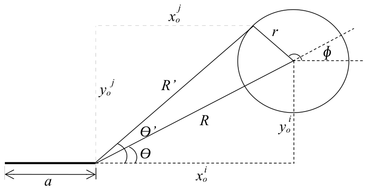
where K I is the stress intensity factor for Mode I, G is the shear modulus, ν is Poisson’s ratio and κ = ( 3 ν ) / ( 1 + ν ) . Polar coordinates were used for integration, in which particles i are located at a distance R from the crack tip and particles j at a distance R as shown in Figure 1, where x o j = x o i + ( y + z ) cos ϕ , y o j = y o i + ( y + z ) sin ϕ . Thus, employing Equations (16) and (17), the displacements for particles i and j are given by the following:
u i = K I 2 G R 2 π cos θ 2 κ 1 + 2 sin 2 θ 2 ,
u j = K I 2 G R 2 π cos θ 2 κ 1 + 2 sin 2 θ 2 ,
v i = K I 2 G R 2 π sin θ 2 κ + 1 2 cos 2 θ 2 ,
v j = K I 2 G R 2 π sin θ 2 κ + 1 2 cos 2 θ 2 .
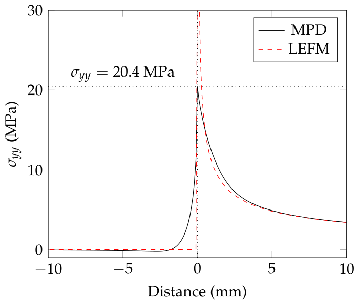
According to LEFM, there is a singularity as R 0 ; similarly, the singularity remains in the present model when R = 0 . However, by performing numerical approximations from the left and from the right ( lim R 0 + σ , lim R 0 σ ), R r (Figure 2), integration can be performed from the crack tip; thus, the stresses in the x and y directions are given by
σ x x = 16 K I ( 27 ν 2 263 ν 10 ) 525 ( ν 2 1 ) 2 π 3 δ ,
τ x y = 16 K I ( 153 ν 2 732 ν + 235 ) 525 ( 1 ν 2 ) 2 π 3 δ ,
τ y x = 8 K I ( 219 ν 2 1336 ν + 405 ) 525 ( ν 2 1 ) 2 π 3 δ ,
σ y y = 32 K I ( 39 ν 2 + 79 ν 100 ) 525 ( ν 2 1 ) 2 π 3 δ .
As an example, consider a single-edge-notched plate subjected to a tensile stress σ of 2 MPa. The notch value a is 30 mm, and the width W is 150 mm. The material parameters are given by E = 18,000 MPa and ν = 0.20. The stress intensity factor for this case is obtained with the following formula:
K I = Y σ π a ,
Y = 2 W π a tan π a 2 W 0.752 + 2.02 a W + 0.37 1 sin π a 3 cos ( π a 2 W ) .
The value of K I obtained was 26.98 MPa-m1/2, and the stress σ y y using Equation (21) is 20.4 MPa. Figure 2 shows a plot of micropolar peridynamic stress σ y y using numerical integration compared to a plot of the same stress using LEFM. In addition, the stress value of 20.4 MPa is shown at the tip of the crack.
On the basis of MPD and the micropolar peridynamic stress, a numerical model was developed, which is explained in the following section.

2.2. Numerical Model

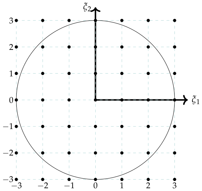
A single-processor computer code was developed, and, in order to maximize its efficiency, the use of matrix operations was prioritized, and loops and logical blocks were minimized; several arrays of stored displacements and material properties were distributed on grids that have one unit of measure. In this model, a material horizon of three times the grid spacing was chosen. Consequently, the stress tensor was calculated using a matrix of material points j with a size of 7 × 7 at each point i (Figure 3).
The geometry and model parameters were distributed in a n × m array, where n is the number of points in x and m is the number of points in the y direction. The rotational stiffness and stiffness matrices were obtained as follows:
k x = [ k x ] n × m , k y = [ k y ] n × m , k z = [ k z ] n × m .
The frequencies were calculated using matrix operations as follows:
ω x = k x m , ω y = k y m .
The mass moment of inertia was defined at each point such that the rotational frequency coincided with the translational frequency,
Δ I = k z ω x 2 , ω z = k z Δ I ,
and the time differential Δ t was chosen such that
ω m a x = m a x ( ω x , ω y , ω z ) , Δ t < 1 ω m a x .
In an implicit linear module, displacements and rotations [ u ] were obtained by inverting the global stiffness matrix [ K ] :
[ u ] = [ K ] 1 [ f e x t ] ,
where [ f e x t ] is the applied force. The initial displacements in x and y were obtained using the expression mentioned above ( [ u ] , [ v ] ) with rotations and stretches.
According to the constitutive model, the forces in all peridynamic links are calculated ( f x i n t , f y i n t ), and the damping forces are initialized and calculated using the following formula:
f d a m = 2 c l Δ v Δ m 3 Δ t ,
where Δ v , Δ m , Δ t are the velocities, mass, and time differentials, respectively, and c l is the translational damping factor. Similarly, for damping moments,
m z d a m = c θ 2 Δ t w z Δ I ,
where c θ and w z are the rotational damping factor and the angular velocity, respectively.
After all forces and moments are determined, the accelerations in the coordinates x and y are calculated using the following expressions:
a x = f x i n t + f x e x t + f x d a m Δ m , a y = f y i n t + f y e x t + f y d a m Δ m ,
where, a x , a y are the accelerations x and y, f x i n t , f y i n t are the internal forces, f x e x t , f y e x t , are the external forces and f x d a m , f y d a m are the damping forces in the x and y, respectively. Similarly, the angular accelerations with
α z = m z i n t + m z e x t + m z d a m Δ I ,
where α z is the angular acceleration, m z i n t , m z e x t , and m z d a m are the internal, external, and damping moments, respectively, and Δ I is the differential of the mass moment of inertia. Thus, velocities, rotations, and displacements are integrated using
v x = v x o + a x Δ t , v y = v y o + a y Δ t ,
u = u o + v x Δ t , v = v o + v y Δ t ,
and
w z = w z o + α z Δ t , θ z = θ z o + w z Δ t ,
where v o , w o , θ o , and u o are the velocities, angular velocities, rotations, and displacements from the initial conditions, respectively. The magnitude of the three accelerations is obtained using
| a | = a x 2 + a y 2 + α z 2 Δ s ,
where Δ s is the grid spacing. If | a | is less than some prescribed minimum acceleration, then a steady-state solution has been achieved, and the results of that load step can be plotted out. This also occurs if the number of steps has reached a maximum value; otherwise, displacements and rotations must be computed again.
The properties and displacements of the material were ordered in 7 × 7 arrays to determine the stresses at the node i (Figure 3). To accelerate the calculation of the stress tensor at all points in the domain, some vectors were previously calculated by computing integrals by Lagrange interpolation. The following 49 × 1 distance vectors were defined: [ ξ 1 ] and [ ξ 2 ] : [ ξ 1 ] = [ 3 , , x j x i , , 3 ] Δ s , [ ξ 2 ] = [ 3 , , y j y i , , 3 ] Δ s , x j , y j , x i , y i are the coordinates of particles j and i, respectively, and Δ s is the grid spacing. Let the matrix [ a ] of 49 × 49 be defined for each element as follows:
a k , i + 7 ( j 1 ) = ξ 1 i 1 ( k ) ξ 2 j 1 ( k ) .
and the matrix [ c p ] is defined as
c i j p = a i j 1 ,
for i = 1 7 , j = 1 7 and k = 1 49 , where a i j is obtained with Equation (31).
Let x ˜ = ( y + z ) cos θ and y ˜ = ( y + z ) sin θ , so that x ˜ and y ˜ are within a radius circle ( y + z ) . Let a vector 1 × 49 [ p ] be defined as
[ p ] = [ x ˜ 0 y ˜ 0 x ˜ 0 y ˜ 1 . . . x ˜ 6 y ˜ 6 ] ,
A coefficient vector [ c u v ] was obtained using Equation (32):
[ c u v ] = [ c p ] [ p ] .
Using Equation (3) and the transformation matrix in Equation (10), the peridynamic link stiffness is given by
[ k ] = [ T ] T [ k ^ ] [ T ] ,
so that the peridynamic force for stresses in the x x direction and displacements in the x direction can be expressed as
[ f x x u ] = k 11 [ c u v ] cos ( θ ) .
Similarly, the material parameters d for x y stresses and displacements in the y direction are calculated as follows:
[ f x y v ] = k 22 [ c u v ] cos ( θ ) .
Thus, material parameters c for x x stresses and displacements in the x direction are calculated using the following equation:
[ c x x u ] = 0 2 π 0 δ 0 δ y [ f x x u ] ( y + z ) d z d y d θ ,
Similarly, x y stresses and displacements of parameters d and in the y direction:
[ d x y v ] = 0 2 π 0 δ 0 δ y [ f x y v ] ( y + z ) d z d y d θ .
For each material point i with coordinates ( p , q ) , displacements, rotations, and material properties for all particles j with coordinates ( r , s ) near each particle i can be represented using the following tensors:
u p q r s s , v p q r s s , θ p q r s s , c p q r s s , d p q r s s ,
for displacements u , v , θ and material properties c , d , where 3 r 3 and 3 s 3 , in which the boundaries were verified to obtain real, physically reasonable values. These tensors were reduced to third-order tensors using 49 nonzero indices instead of r and s.
u p q k s , v p q k s , θ p q k s , c p q k s , d p q k s .
The material parameters c and d can be represented as the following first-order tensors:
c k u x x , c k u y y , c k u x y , c k u y x , c k v x x , c k v y y , c k v x y , c k v y x , d k u x x , d k u y y , d k u x y , d k u y x , d k v x x , d k v y y , d k v x y , d k v y x ,
and the following third-order tensors for x x stresses are computed for displacements in the x direction (u):
s p q k u x x = c p q k s c k u x x + d p q k s d k u x x , ( No contraction ; k is now a free index ) ,
and the same stresses in the y direction (v):
s p q k v x x = c p q k s c k v x x + d p q k s d k v x x , ( No contraction ; k is now a free index ) .
Displacements at each point ( p , q ) are represented as first-order tensors u k and v k , so the stresses are computed using the following Equations.
σ p q x x = s p q k u x x u k + s p q k v x x v k
σ p q y y = s p q k u y y u k + s p q k v y y v k
σ p q x y = s p q k u x y u k + s p q k v x y v k
σ p q y x = s p q k u y x u k + s p q k v y x v k .
At each point ( p , q ) , σ x x , σ y y , σ x y , σ y x are represented using matrices for two-dimensional plane stress problems, such as
[ σ ] = σ x x σ x y σ y x σ y y ,
where [ σ ] is not symmetric for most micropolar peridynamic problems. One way to ensure symmetry is by defining σ ¯ x y = ( σ x y + σ y x ) / 2 ; the principal stress can be calculated with Equation (39), and different failure criteria can be applied to plane stress problems.
For comparison purposes, a two-dimensional FEM single-processor computer code was also developed. In this model, quadrilateral elements of one unit of measure were used with three-by-three Gauss points for each element. Examples using these schemes are explained in the following subsections.

2.2.1. Circular Hole Plate Subjected to Tensile Stress

A concrete plate with a circular hole in the center subjected to tensile stress was simulated with the micropolar peridynamic model and the finite element model.
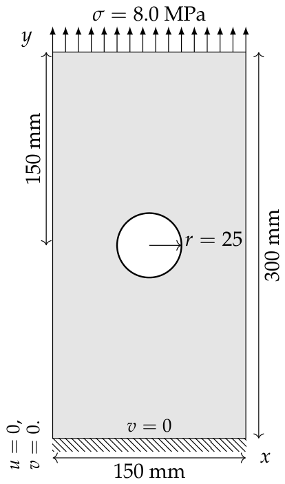
The geometry and boundary conditions are described in Figure 4. The material properties are an elastic modulus E = 18,000 MPa and a Poisson’s ratio ν = 0.20 . The plate thickness is 50 mm, the mesh consists of 150 × 300 = 45,000 particles, and the material horizon is δ = 3 mm. For the FEM code, 150 × 300 = 45,000 quadrilateral elements were also used. The applied tensile stress σ was 8.0 MPa.
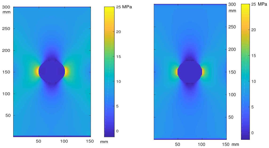
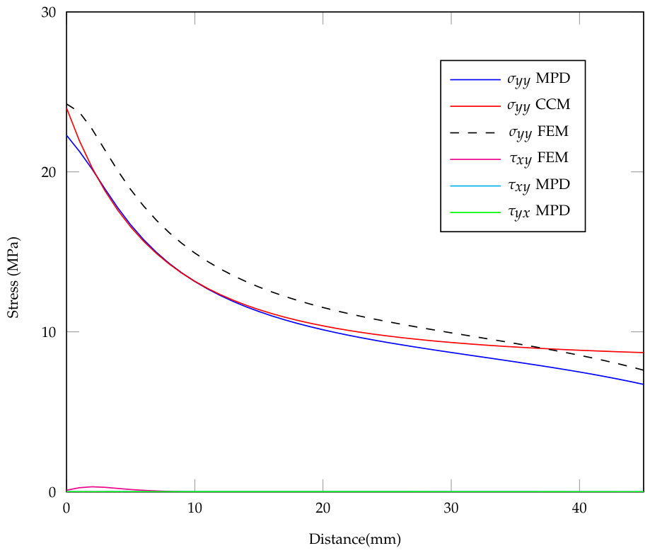
Figure 5 shows the stress field plots in MPa ( σ y y ) using the finite element model and the micropolar peridynamic model, respectively. Figure 6 shows the stress plots at the right edge of the circular hole ( y = 150 mm) using the last two models and the analytical solution (CCM). These plots show close agreement between MPD and CCM stresses.

2.2.2. Single-Edge-Notched Plate Subjected to Tension

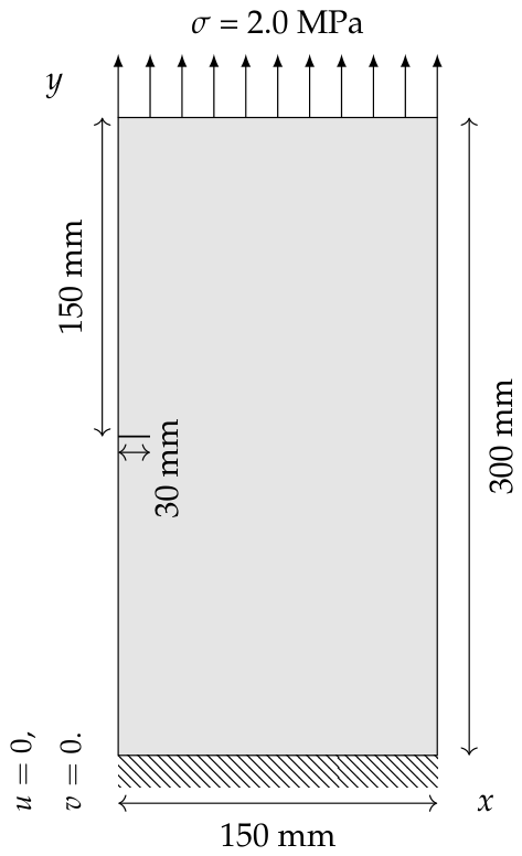
A single-edge-notched concrete plate subjected to plane stress loading was simulated using the models described above. The geometry of the model and the boundary conditions are described in Figure 7. The modulus of elasticity is E = 18,000 MPa, and the Poisson’s ratio ν = 0.20 . The thickness of the plate is 50 mm, and the material horizon is 3 mm. The number of quadrilateral elements and particles was 150 × 300 for the finite element and micropolar peridynamic models, respectively.
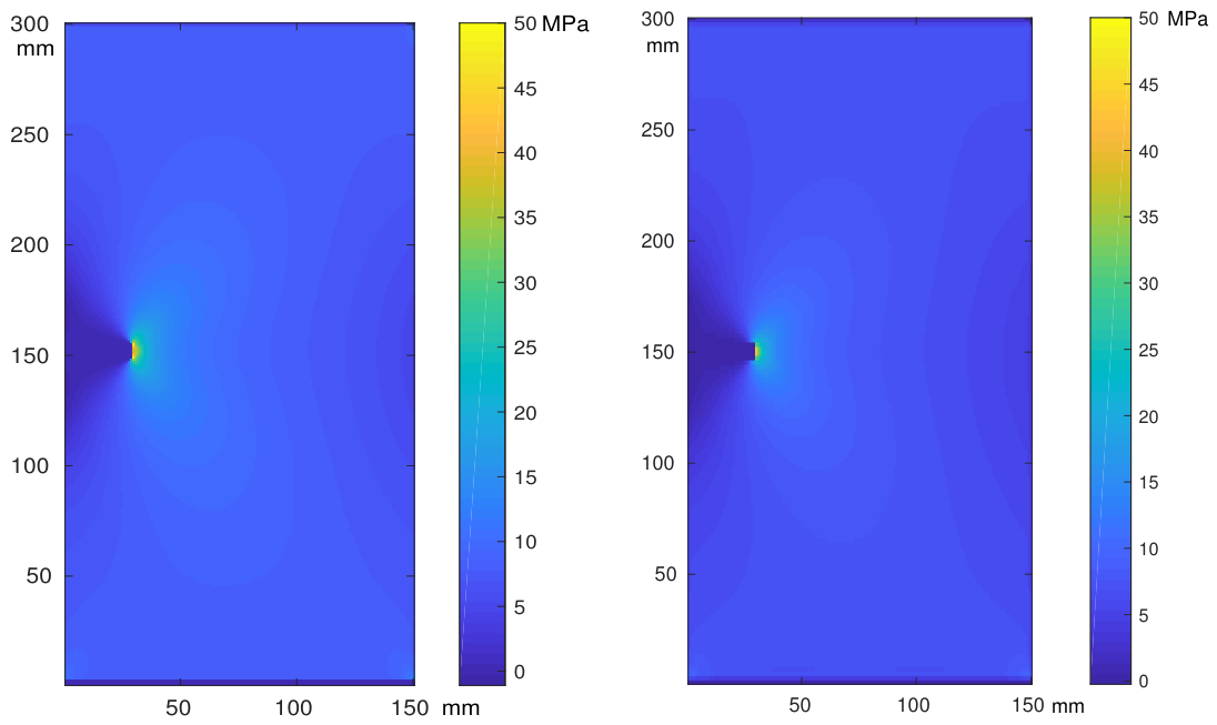
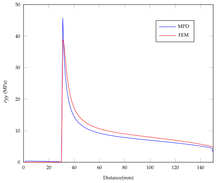
Figure 8 shows the stress field plots in MPa ( σ y y ) using FEM and MPD models, and Figure 9 shows a comparison of the same stress in the middle of the plate using MPD and FEM.

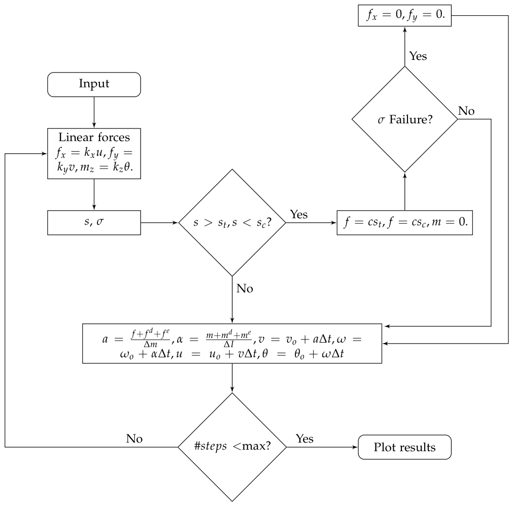
2.3. Damage Model for Concrete

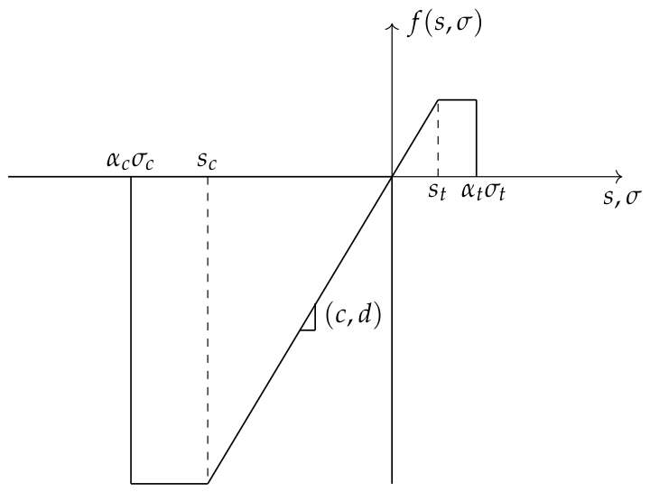
A concrete damage model was implemented using the single-processor code described above. Based on Figure 10 and an explicit dynamic relaxation method, an implicit linear elastic model was used to find the load required to break the first bond. Subsequently, a nonlinear explicit dynamic relaxation model was used. A nonlinear bond-based damage function for concrete was obtained by calculating the forces between the particles i and j using a microelastic damage function. Nonlinear microelastic damage models were previously developed in [9], where the connection force changed if the maximum stretch exceeded some prescribed values. Figure 11 shows an example of a microelastic damage model for concrete structures, where softening behavior was considered. The force function is a function of the stretch s between the particles i and j as well as the stress σ at node i. In this model, the link remains linearly elastic as long as its stretch s does not fall below the compressive stretch limit s c and does not exceed the tensile stretch limit s t . The tensile peridynamic force remains constant after this value and before s c , and the compressive force is constant. If the value of α t σ t exceeds another specified value, the force at node i decreases to zero. Similarly, if α c σ c decreases to some other value, the force on the particle i also falls to zero. In this case, σ t and σ c are the maximum tensile stress and the compressive strength at point i, respectively, and α c , α t are the material parameters. These factors α need to be greater than one because once one link is broken, the peridynamic stress should not consider the force of that broken link. However, considering the decrease in stress due to broken links, more computing time will be required for subsequent calculations. Thus, with these material parameters, the numerical value of the peridynamic stress is approximately equal to the real value of the stress at any point within the domain.
For each simulation, the mesh size, applied forces, material parameters, and dynamic relaxation parameters were chosen. Once the forces are obtained in all links, the critical link is located and the load factor is calculated to break this link. The load was increased using a prescribed load increment factor, and the peridynamic forces and moments were calculated. In addition, the stretch intervals were recalculated using this increase in load. Once the initial loads and displacements are obtained, the stress tensor is calculated at each point. The process of computing the stress tensor is described in Section 2.2.
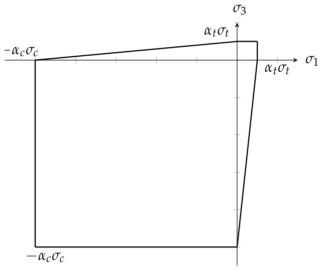
Using the Mohr failure criterion, if the maximum or minimum stresses ( σ 1 , σ 3 ) fall outside the failure surface (Figure 12), all peridynamic links that attach the particle i drop to zero (Figure 11).
Once a peridynamic link fails, the peridynamic stress changes. For efficiency purposes, the stiffness of all the links attached to the particle i is not changed; therefore, the material parameters α c and α t should take into account the decrease in stress due to progressive link failure.
As mentioned in Section 1, many peridynamic studies treat the material horizon as a free parameter. This parameter is generally expressed as a function of the modulus of elasticity, stretch, maximum stress, and fracture energy [16,41], in which the material horizon of a typical concrete is on the order of 800 mm.
Using the equations described in Section 2.1, the material horizon can be expressed as a function of the fracture toughness, the maximum tensile stress, and the Poisson’s ratio. Therefore, if failure occurs ( K I = K I c ), the material horizon δ can be expressed using the maximum tensile stress of Equations (18)–(21) as follows:
δ = f p K I c σ t 2 ,
where f p is a function of π and Poisson’s ratio ν . For example, for a Poisson’s ratio of 0.22, f p = 0.05618899.
Applications to specific problems are discussed in the following section.

3. Results

In this section, plane stress simulations are evaluated using plain concrete problems and compared with physical results from the laboratory.

3.1. Double-Edge-Notched Specimen Subjected to Uniaxial Tension

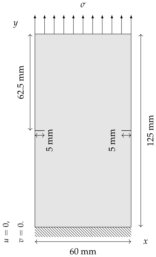
A double-edge-notched plain concrete specimen subjected to tensile stress was analyzed using the method described in Section 2.2. These plates were modeled using extended FEM in [44], and some experiments were carried out by [45] in 1991. Using the material properties reported in [44], the concrete modulus of elasticity was 18.0 GPa, σ c = 30 MPa, and σ t = 3.2 MPa. The geometry and boundary conditions are shown in Figure 13, and the following equation was used to obtain K I c [46]:
K I = f a W σ π a ,
f a W = 1.122 0.561 ( a / W ) 0.205 ( a / W ) 2 0.190 ( a / W ) 4 1 ( a / W ) ,
where W is the semi-width of the plate, a is the depth of the notch, and σ is the applied maximum stress of 3.2 MPa. Thus, for a thickness of 50 mm, the value of K I c was 0.45 MPa·m1/2. To model the notches, the material in the notch regions was assigned significantly weaker than that of the surrounding concrete. Using Equation (40), where an assumed value of the Poisson’s ratio of 0.22 was incorporated, the value of the material horizon δ is 0.0015 m, which is 1.5 mm. According to Section 2.2, δ is three times the grid spacing; therefore, the model grid spacing is 0.5 mm, so a mesh size of 120 × 250 was used. The tension ( s t ) and compression ( s c ) stretches were 0.00018 and 0.0018, respectively. After calibrating the values of α , the values of α c and α t were 5.0 and 2.5, respectively.
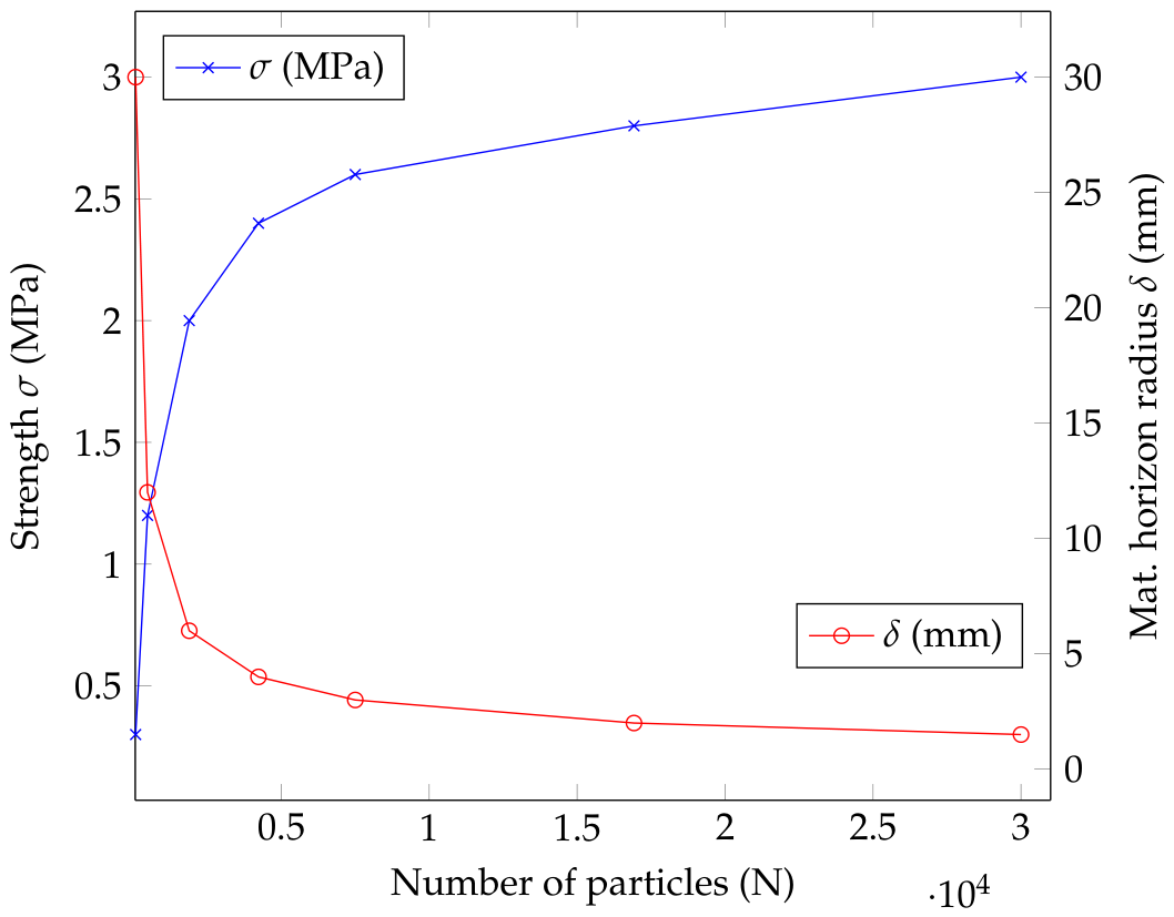
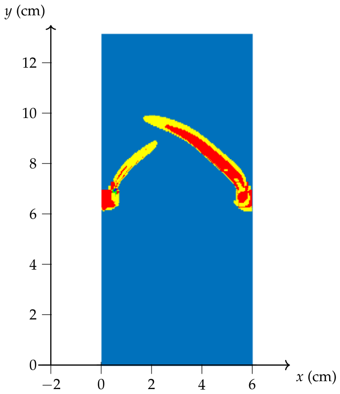
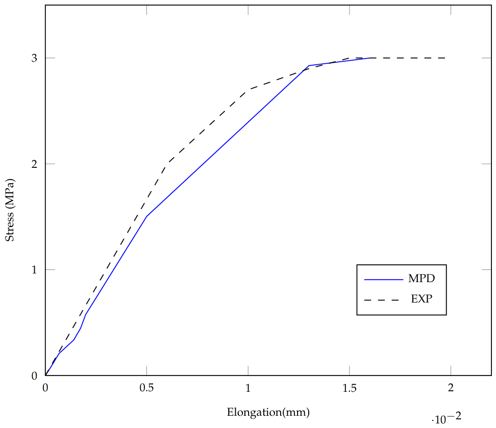
Figure 14 shows the crack trajectories of this plate using MPD, and Figure 15 shows the stress–elongation curves obtained using this model, compared to the experiment reported by Hordijk [45]. To ensure reliability of the results, a strength graph and the size of the material horizon versus the number of particles are shown in Figure 16, where the material horizon/discretization ratio ( m = δ / Δ x ) was kept constant ( m = 3).

3.2. Four-Point Single-Edge-Notched Beam Subjected to Flexure

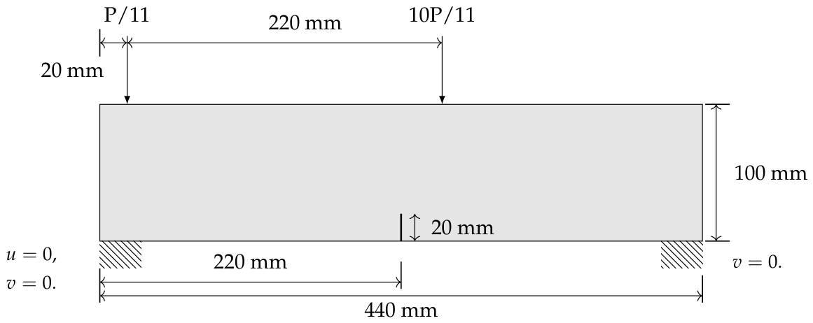
A single-edge-notched four-point loaded plain concrete beam was analyzed with the method described in Section 2.2. Notched beams with four-point loads have been modeled using both the finite element method and peridynamics in [44,47]. The properties of concrete were E = 35.0 GPa, σ t = 3 MPa, and σ c = 45 MPa. Using a Poisson’s ratio of 0.2 and assuming a typical fracture toughness value of 1.4 MPa·m1/2, the value of δ according to Equation (40) is 3.3 mm, so the grid spacing for this model was 1.0 mm. Figure 17 shows the configuration of the problem. After calibrating the values of α , the values of α c and α t were 2.0 and 1.5, respectively.
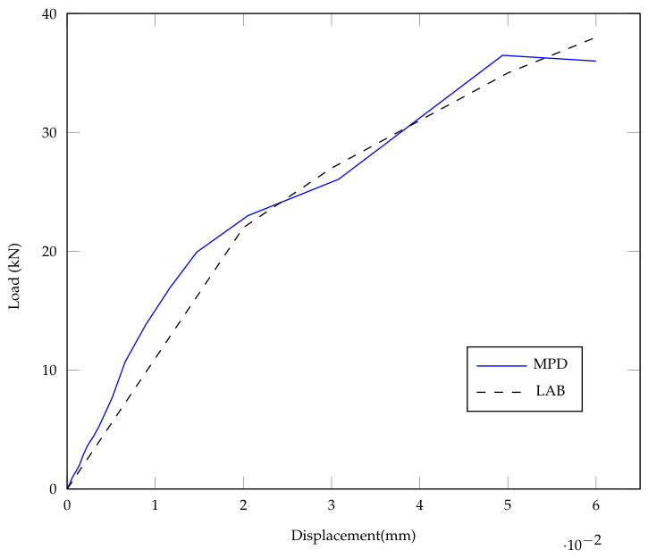
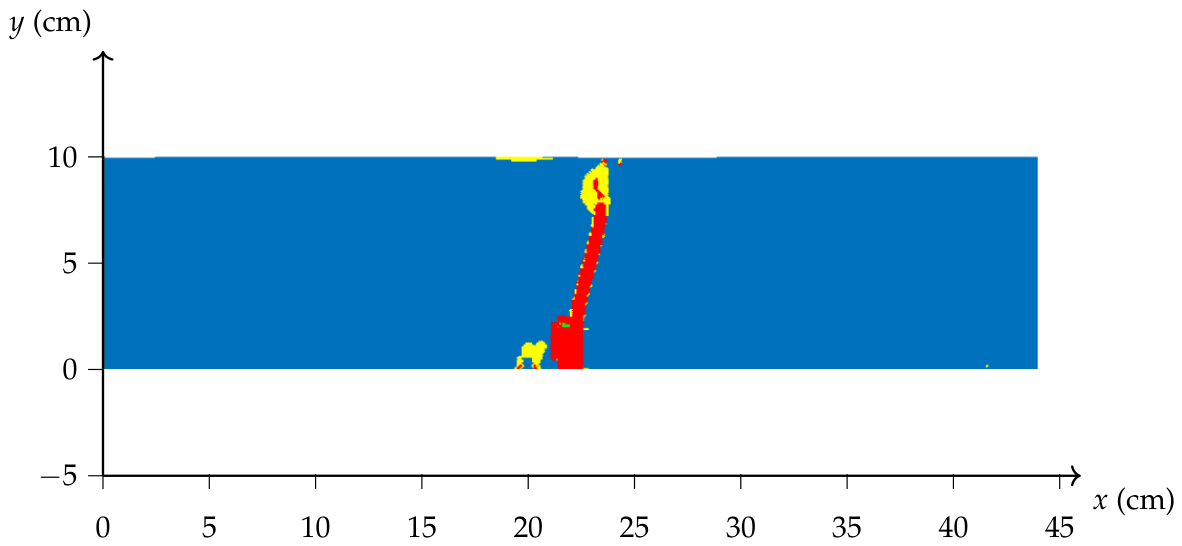
Figure 18 and Figure 19 show the crack trajectory and the load–deflection curve of this model using the scheme shown above. This path coincides with those found in [44,47] and is in agreement with the experimental results reported by Tejchman and Bobinski [44].

3.3. Three-Point Single-Edge-Notched Beam Subjected to Flexure

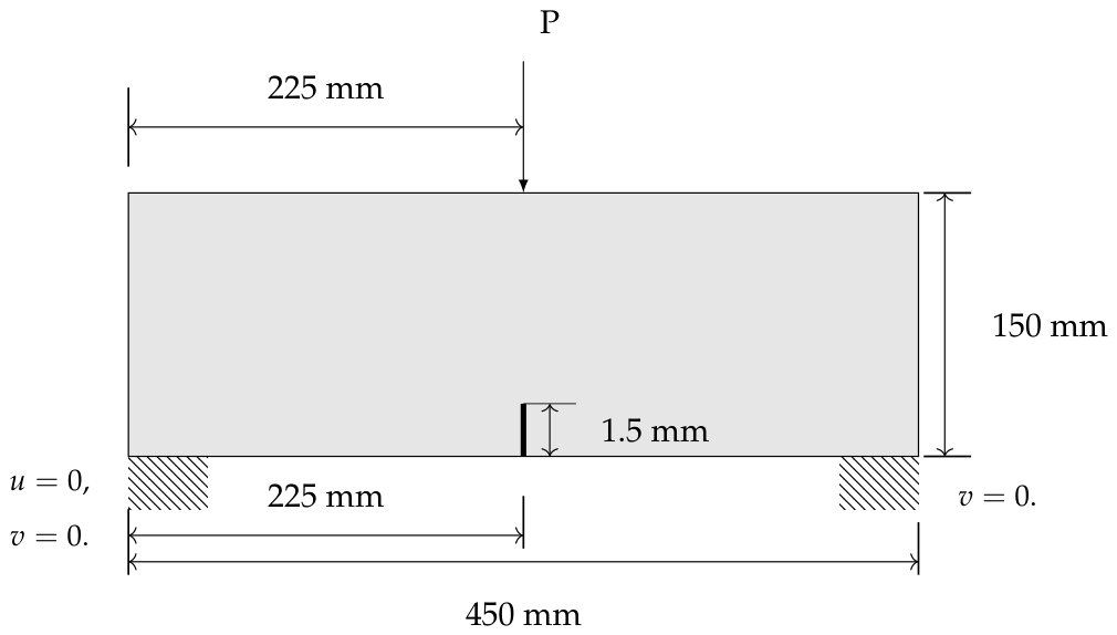
Based on the methodology described above, a three-point plain concrete beam was simulated using micropolar peridynamics and compared with laboratory results. The geometry and boundary conditions are shown in Figure 20. According to laboratory tests, the concrete modulus of elasticity was 21.1 GPa, with σ c = 20 MPa and σ t = 2.0 MPa. Using the following equation [43]:
K I = P B W f a W ,
f a W = 3 S W a W 1.99 a W 1 a W 2.15 3.93 a W + 2.7 a W 2 , 2 1 + 2 a W 1 a W 3
where W is the width of the beam, S is the span, a is the depth of the notch, B is the thickness of the beam (150 mm), and P is the maximum applied load (11.7 kN), the obtained value of K I c was 0.51 MPa·m1/2. Employing Equation (40) with a Poisson’s ratio of 0.22, the value of the material horizon δ is 0.0033 m, which is approximately 3 mm, and in this case, the model grid spacing is 1 mm. The tension ( s t ) and compression ( s c ) stretches were 0.0001 and 0.001, respectively, and the values of α c and α t were 5.0 and 2.0, respectively.
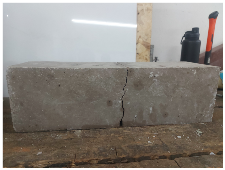
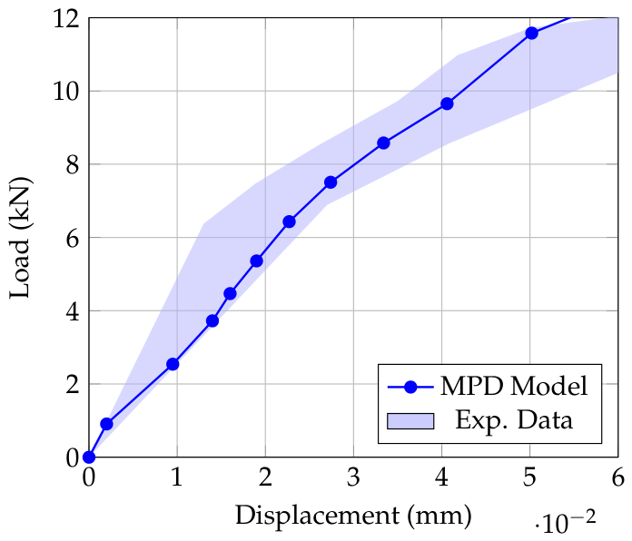
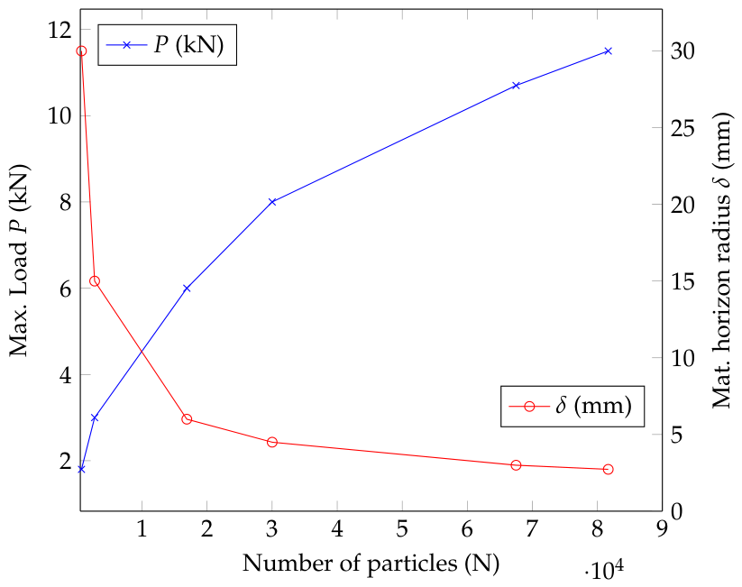
Figure 21 shows the crack path of this beam using the aforementioned model, and Figure 22 shows the crack of the three-point loaded beam after a physical test. This path agrees with those previously reported in [44] and the crack observed in the laboratory test. Figure 23 shows the load–displacement curve obtained in the laboratory compared to the one obtained with the model. In addition, a plot of the maximum load and the size of the material horizon is shown in Figure 24 using a value of m = 3.
Figure 16 and Figure 24 demonstrate the independence of the mesh. Implementing the MPD model with stress and stretch failure criteria mitigates spurious boundary effects, ensuring robust spatial convergence.

4. Discussion

To validate the efficacy of our proposed micropolar peridynamic model with stress and stretch failure criteria, we conducted a comparative analysis against existing peridynamic models. The evaluation was performed on three critical parameters: Poisson’s ratio restriction, failure criteria, computational overhead, and material horizon parameters. These peridynamic models fall into three main categories: nonordinary state-based, bond-based with nonlocal stresses, and micropolar with local stresses. Our ongoing study uniquely advances a micropolar model with nonlocal stress derivation.
  • Nonordinary State-Based Peridynamics (NOSB-PD). Unlike bond-based peridynamics, NOSB-PD incorporates classical stress and strain tensors into its constitutive framework. NOSB-PD overcomes Poisson’s ratio restriction. However, the nonlocal integration scheme used in NOSB-PD can produce spurious nonzero energy modes. In addition, evaluating nonlocal interactions in a designated particle neighborhood requires significantly more memory and computational time [48,49,50].
  • Bond-Based Peridynamics with Nonlocal Stresses. Bond-based peridynamics with a nonlocal stress calculation eliminates physically impossible, theoretically infinite stresses at crack tips. Although simpler to implement than state-based alternatives, it introduces moderate computational overhead. Furthermore, it requires a free-parameter horizon size and restricts Poisson’s ratio to 1 / 3 in two dimensions and to 1 / 4 in three dimensions [30,51,52].
  • Micropolar Peridynamics with Local Stresses. Incorporating moments and rotational degrees of freedom into micropolar peridynamics with a local stress calculation enables modeling materials with flexible Poisson’s ratios. Although parameter calibration requires experimental testing, this approach offers simpler implementation and moderate computational costs compared to state-based models. The material horizon is a free parameter, and it remains susceptible to typical boundary effects [20,24,36,37].
  • Micropolar Peridynamics with Nonlocal Stresses. This study implemented a micropolar peridynamic framework that utilizes both stress and stretch failure criteria to solve plane stress concrete problems. By employing a nonlocal stress tensor, the model achieves moderate computational efficiency while avoiding the complexity of state-based alternatives. Unlike traditional approaches that treat the material horizon as an arbitrary constant, this research links the horizon directly to physical properties such as Poisson’s ratio, material strength, and fracture toughness. The implementation of the model mitigates spurious boundary effects, ensuring spatial convergence.

5. Conclusions

A novel micropolar peridynamic framework was developed for two-dimensional concrete structures. By accounting for material rotations and moment densities, it simulates plane stress models. The approach seamlessly captures fractures without special techniques and defines the material horizon based on concrete properties, ensuring mesh-independent results and accurate spatial convergence. The new framework introduces several key features and advantages over classical and standard peridynamic models:
  • It uses stress- and stretch-based criteria to naturally handle cracking, avoiding the mathematical singularities at discontinuities that plague classical tensor models.
  • Instead of treating the interaction radius purely as an abstract parameter, the model explicitly defines it based on the material’s strength, fracture toughness, and Poisson’s ratio.
  • It establishes direct mathematical equivalence to classical linear elastic stress–strain tensors and mitigates spurious boundary effects while matching experimental testing data.
Calculating the Lehoucq–Silling stress tensor and similar discontinuous stress definitions is notoriously time-consuming. Future studies will integrate the proposed framework with elasto-plastic models and large deformation theories in connection with finite element methods and remeshing algorithms. Although integrating remeshing algorithms with finite element methods offers a practical workaround, one must carefully monitor the size and spatial proximity of each element when computing peridynamic stress tensors to ensure accuracy. Furthermore, by leveraging parallel computing, full three-dimensional models will be analyzed, and two-dimensional simulations will be accelerated.

Author Contributions

Conceptualization, N.S.-S. and G.K.I.-T.; methodology, N.S.-S.; software, J.P.A.-M.; validation, A.C.B.-A., G.K.I.-T. and L.G.-M.; formal analysis, N.S.-S.; investigation, N.S.-S.; resources, A.C.B.-A.; data curation, L.G.-M.; writing—original draft preparation, N.S.-S.; writing—review and editing, A.C.B.-A. and J.P.A.-M.; visualization, A.C.B.-A. and G.K.I.-T. All authors have read and agreed to the published version of the manuscript.

Funding

This research was funded by the University of Sonora, project number USO316010116.

Data Availability Statement

Calculation of integrals depicted in Section 2.1 can be found in https://github.com/nsau71/quasi-stiffnesses (accessed 11 July 2026).

Acknowledgments

Special thanks to the Faculty and Staff of the Experimental Engineering Laboratory, Mario Garcia, Luis Torres, and students.

Conflicts of Interest

The authors declare no conflicts of interest.

Abbreviations

The following abbreviations are used in this manuscript:
CCMClassical continuum mechanics
FEMFinite element method
MPDMicropolar peridynamics
LEFMLinear elastic fracture mechanics

References

  1. Silling, S.A. Reformulation of elasticity theory for discontinuities and long-range forces. J. Mech. Phys. Solids 2000, 48, 175–209. [Google Scholar] [CrossRef] [Scilit]
  2. Gerstle, W.; Sau, N. Proceedings of the Fifth International Conference on Fracture Mechanics of Concrete Structures (FRAMCOS 5), Vail, CO, USA, 12–16 April 2004; Taylor & Francis: Abingdon, UK, 2004. [Google Scholar] [CrossRef] [Scilit]
  3. Huang, D.; Zhang, Q.; Qiao, P.Z. Damage and progressive failure of concrete structures using non-local peridynamic modeling. Sci. China Technol. Sci. 2011, 54, 591–596. [Google Scholar] [CrossRef] [Scilit]
  4. Demmie, P.N.; Silling, S.A. An approach to modeling extreme loading of structures using peridynamics. J. Mech. Mater. Struct. 2007, 2, 1921–1945. [Google Scholar] [CrossRef] [Scilit]
  5. Silling, S.A.; Askari, E. Peridynamic modeling of impact damage. In Proceedings of the American Society of Mechanical Engineers, Pressure Vessels and Piping Division (Publication) PVP, San Diego, CA, USA, 25–29 July 2004; Volume 489, pp. 197–205. [Google Scholar]
  6. Shen, F.; Zhang, Q.; Huang, D. Damage and failure process of concrete structure under uniaxial compression based on peridynamics modeling. Math. Probl. Eng. 2013, 2013, 631074. [Google Scholar] [CrossRef] [Scilit]
  7. Huang, D.; Lu, G.D.; Wang, M.W. Peridynamic modeling of concrete structures. Appl. Mech. Mater. 2014, 638, 1725–1729. [Google Scholar]
  8. Huang, D.; Lu, G.; Qiao, P. An improved peridynamic approach for quasi-static elastic deformation and brittle fracture analysis. Int. J. Mech. Sci. 2015, 94-95, 111–122. [Google Scholar] [CrossRef] [Scilit]
  9. Gerstle, W.; Sau, N.; Aguilera, E. Micropolar peridynamic modeling of concrete structures. In Proceedings of the 6th International Conference on Fracture Mechanics of Concrete and Concrete Structures—Fracture Mechanics of Concrete and Concrete Structures, Catania, Italy, 17–22 June 2007; pp. 475–481. [Google Scholar]
  10. Silling, S.A.; Epton, M.; Weckner, O.; Xu, J.; Askari, E. Peridynamic states and constitutive modeling. J. Elast. 2007, 88, 151–184. [Google Scholar] [CrossRef] [Scilit]
  11. Yang, D.; He, X.; Yi, S.; Liu, X. An improved ordinary state-based peridynamic model for cohesive crack growth in quasi-brittle materials. Int. J. Mech. Sci. 2019, 153, 402–415. [Google Scholar] [CrossRef] [Scilit]
  12. Zhang, Q.; Xia, X. Elastoplastic constitutive modeling for reinforced concrete in ordinary state-based Peridynamics. J. Mech. 2020, 36, 799–811. [Google Scholar] [CrossRef] [Scilit]
  13. Bazilevs, Y.; Behzadinasab, M.; Foster, J.T. Simulating concrete failure using the Microplane (M7) constitutive model in correspondence-based peridynamics: Validation for classical fracture tests and extension to discrete fracture. J. Mech. Phys. Solids 2022, 166, 104947. [Google Scholar] [CrossRef] [Scilit]
  14. Lubarda, A. Micropolar Elasticity. In Mechanics of Solids and Materials; Asaro, R., Lubarda, V., Eds.; Cambridge University Press: Cambridge, UK, 2006; pp. 375–406. [Google Scholar]
  15. Lakes, R.S. Experimental methods for study of Cosserat elastic solids and other generalized elastic continua. In Continuum Models for Materials with Microstructures; Mühlhaus, H., Ed.; Wiley: New York, NY, USA, 1995; pp. 1–22. [Google Scholar]
  16. Gerstle, W.; Sau, N.; Silling, S. Peridynamic modeling of concrete structures. Nucl. Eng. Des. 2007, 237, 1250–1258. [Google Scholar] [CrossRef] [Scilit]
  17. Gerstle, W.H.; Sau, N.; Sakhavand, N. On peridynamic computational simulation of concrete structures. In Proceedings of the American Concrete Institute, ACI Special Publication, New York, NY, USA, 8–12 November 2009; pp. 245–264. [Google Scholar]
  18. Roy Chowdhury, S.; Masiur Rahaman, M.; Roy, D.; Sundaram, N. A micropolar peridynamic theory in linear elasticity. Int. J. Solids Struct. 2015, 59, 171–182. [Google Scholar] [CrossRef] [Scilit]
  19. Diana, V.; Casolo, S. A bond-based micropolar peridynamic model with shear deformability: Elasticity, failure properties and initial yield domains. Int. J. Solids Struct. 2019, 160, 201–231. [Google Scholar] [CrossRef] [Scilit]
  20. Diana, V.; Labuz, J.F.; Biolzi, L. Simulating fracture in rock using a micropolar peridynamic formulation. Eng. Fract. Mech. 2020, 230, 106985. [Google Scholar] [CrossRef] [Scilit]
  21. Diana, V.; Ballarini, R. Crack kinking in isotropic and orthotropic micropolar peridynamic solids. Int. J. Solids Struct. 2020, 196-197, 76–98. [Google Scholar] [CrossRef] [Scilit]
  22. Guo, X.; Chen, Z.; Chu, X.; Wan, J. A plane stress model of bond-based Cosserat peridynamics and the effects of material parameters on crack patterns. Eng. Anal. Bound. Elem. 2021, 123, 48–61. [Google Scholar] [CrossRef] [Scilit]
  23. Zhang, Y.; Yang, X.; Wang, X.; Zhuang, X. A micropolar peridynamic model with non-uniform horizon for static damage of solids considering different nonlocal enhancements. Theor. Appl. Fract. Mech. 2021, 113, 102930. [Google Scholar] [CrossRef] [Scilit]
  24. Yu, H.; Chen, X. A viscoelastic micropolar peridynamic model for quasi-brittle materials incorporating loading-rate effects. Comput. Methods Appl. Mech. Eng. 2021, 383, 113897. [Google Scholar] [CrossRef] [Scilit]
  25. Lei, J.; Lu, Y.; Sun, Y.; Jiang, S. A micropolar damage model for size-dependent concrete fracture problems and crack propagation simulated by PDDO method. Eng. Anal. Bound. Elem. 2024, 167, 105882. [Google Scholar] [CrossRef] [Scilit]
  26. Cauchy, A.L. De la pression ou tension dans un corps solide. In Exercises de Mathématiques; Chez de Bure Frères: Paris, France, 1827; Volume 2, pp. 60–81. [Google Scholar]
  27. Kirchhoff, G. Über die Gleichungen des Gleichgewichts eines elastischen Körpers bei beliebiger Formänderung. Ann. Phys. 1852, 162, 321–347. [Google Scholar]
  28. Lehoucq, R.B.; Silling, S.A. Force flux and the peridynamic stress tensor. J. Mech. Phys. Solids 2008, 56, 1566–1577. [Google Scholar] [CrossRef] [Scilit]
  29. Fallah, A.S.; Giannakeas, I.N.; Mella, R.; Wenman, M.R.; Safa, Y.; Bahai, H. On the computational derivation of bond-based peridynamic stress tensor. J. Peridynamics Nonlocal Model. 2020, 2, 352–378. [Google Scholar] [CrossRef] [Scilit]
  30. Ballarini, R.; Diana, V.; Biolzi, L.; Casolo, S. Bond-based peridynamic modelling of singular and nonsingular crack-tip fields. Meccanica 2018, 53, 3495–3515. [Google Scholar] [CrossRef] [Scilit]
  31. Yang, J.; Komvopoulos, K. A stress analysis method for molecular dynamics systems. Int. J. Solids Struct. 2020, 193–194, 98–105. [Google Scholar] [CrossRef] [Scilit]
  32. Li, J.; Li, S.; Lai, X.; Liu, L. Peridynamic stress is the static first Piola–Kirchhoff Virial stress. Int. J. Solids Struct. 2022, 241, 111478. [Google Scholar] [CrossRef] [Scilit]
  33. Adhikari, B.; Li, D.; Han, Z. A Deformation-Based Peridynamic Model: Theory and Application. Buildings 2025, 15, 1931. [Google Scholar] [CrossRef] [Scilit]
  34. Ren, H.; Zhuang, X.; Zhu, H.; Rabczuk, T. Variational damage model: A novel consistent approach to fracture. Comput. Struct. 2024, 305, 107518. [Google Scholar] [CrossRef] [Scilit]
  35. Duan, Y.; Ren, H.; Bie, Y.; Zhuang, X.; Rabczuk, T. A unified variational damage model and an efficient length scale insensitive phase-field model. J. Mech. Phys. Solids 2026, 208, 106494. [Google Scholar] [CrossRef] [Scilit]
  36. Chen, X.; Yu, H. A novel micropolar peridynamic model for rock masses with arbitrary joints. Eng. Fract. Mech. 2023, 281, 109089. [Google Scholar] [CrossRef] [Scilit]
  37. Zhang, N.; Wang, Z.W.; Li, Y.; Gu, Q. A novel micropolar peridynamic damage model for concrete components implemented in OpenSees. Eng. Struct. 2026. Online Version of Record. [Google Scholar] [CrossRef] [Scilit]
  38. Zeng, Z.; Zhang, X. A novel peridynamics refinement method with dual-horizon peridynamics. Eng. Comput. 2025, 41, 2025. [Google Scholar]
  39. Ren, H.; Zhuang, X.; Cai, Y.; Rabczuk, T. Dual-horizon peridynamics. Int. J. Numer. Methods Eng. 2016, 108, 1451–1476. [Google Scholar] [CrossRef] [Scilit]
  40. Bezem, K.; Haeri, S.; TerMaath, S. A Dual-Horizon Peridynamics–Discrete Element Method Framework for Efficient Short-Range Contact Mechanics. Modelling 2025, 6, 131. [Google Scholar] [CrossRef] [Scilit]
  41. Silling, S.; Askari, E. A meshfree method based on the peridynamic model of solid mechanics. Comput. Struct. 2005, 83, 1526–1535. [Google Scholar] [CrossRef] [Scilit]
  42. Pijaudier-Cabot, G.; Toussaint, D.; Pathirage, M.; Cusatis, G. The Role of the Horizon in Modeling Failure due to Strain and Damage Localization with Peridynamics. J. Eng. Mech. 2024, 150, 04024037. [Google Scholar] [CrossRef] [Scilit]
  43. Anderson, T.L. Fracture Mechanics: Fundamentals and Applications, 4th ed.; CRC Press: Boca Raton, FL, USA, 2017. [Google Scholar] [CrossRef] [Scilit]
  44. Tejchman, J.; Bobiński, J. Continuous and Discontinuous Modelling of Fracture in Plain Concrete Under Monotonic Loading BT—Continuous and Discontinuous Modelling of Fracture in Concrete Using FEM; Springer: Berlin/Heidelberg, Germany, 2013; pp. 109–162. [Google Scholar]
  45. Hordijk, D.A. Materials Science, Engineering. In Proceedings of the Local Approach to Fatigue of Concrete, Delft, The Netherlands, 29 October 1991. [Google Scholar]
  46. Tada, H.; Paris, P.C.; Irwin, G.R. The Stress Analysis of Cracks Handbook, 3rd ed.; ASME Press: New York, NY, USA, 2000. [Google Scholar] [CrossRef] [Scilit]
  47. Yang, D.; He, X.; Zhu, J.; Bie, Z. A novel damage model in the peridynamics-based cohesive zone method (PD-CZM) for mixed mode fracture with its implicit implementation. Comput. Methods Appl. Mech. Eng. 2021, 377, 113721. [Google Scholar] [CrossRef] [Scilit]
  48. Gong, B.; Song, Y.; Zhang, L.; Chao, W. Non-ordinary state-based peridynamics model for rock crack propagation: A combined stress-energy fracture method. Sci. Rep. 2026, 16, 40833. [Google Scholar] [CrossRef] [Scilit] [PubMed]
  49. Zhu, T.; Wu, Y.; Zhi, P.; Zhu, P.; Bai, M.; Qi, C. Non-Ordinary State-Based Peridynamics Simulation for Crack Propagation of 3D-Printed Fiber-Reinforced Concrete Beam Under Bending. Materials 2026, 16, 1379. [Google Scholar] [CrossRef] [Scilit]
  50. Li, P.; Hao, Z.; Zhen, W. A stabilized non-ordinary state-based peridynamic model. Comput. Methods Appl. Mech. Eng. 2018, 339, 262–280. [Google Scholar] [CrossRef] [Scilit]
  51. Ignatev, M.; Oterkus, E. Remote stress fracture criterion in peridynamics. Eng. Comput. 2025, 41, 3169–3192. [Google Scholar] [CrossRef] [Scilit]
  52. Song, Z.; Wang, G.; Lu, D.; Zhou, X.; Rabczuk, T.; Du, X. A modeling method of failure for concrete considering the stress state in peridynamics. Int. J. Solids Struct. 2025, 320, 113536. [Google Scholar] [CrossRef] [Scilit]
Figure 1. Location of particles i and j used in the calculation of the micropolar peridynamic stress tensor near the crack tip.
Applmech 07 00058 g001
Figure 2. Plot of stress σ y y versus distance from the crack tip using MPD and LEFM.
Applmech 07 00058 g002
Figure 3. Particle configuration for numerical calculation of the peridynamic stress tensor.
Applmech 07 00058 g003
Figure 4. Boundary conditions and dimensions of a plate with a circular hole at the center.
Applmech 07 00058 g004
Figure 5. σ y y stress using FEM and MPD models for the plate with a circular hole.
Applmech 07 00058 g005
Figure 6. Plot of σ y y , τ x y , and τ y x stresses versus distance from the right edge of the circular hole at y = 150 mm using MPD, FEM and CCM models.
Applmech 07 00058 g006
Figure 7. Boundary conditions and dimensions of the single-edge-notched plate subjected to tension.
Applmech 07 00058 g007
Figure 8. σ y y stress using FEM and MPD models for the SENT plate.
Applmech 07 00058 g008
Figure 9. Plot of σ y y stress versus distance from the right edge of the plate at y = 150 mm using MPD and FEM models.
Applmech 07 00058 g009
Figure 10. Numerical model flowchart for concrete structures.
Applmech 07 00058 g010
Figure 11. Microelastic damage function for concrete structures.
Applmech 07 00058 g011
Figure 12. Mohr–Coulomb failure criterion.
Applmech 07 00058 g012
Figure 13. Boundary conditions and dimensions of the double-edge-notched specimen subjected to tension.
Applmech 07 00058 g013
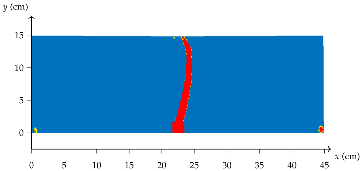
Figure 14. Simulation of a double-edge-notched concrete specimen in tension. Blue signifies no damage, yellow indicates links above the critical stretch s > s t , and red designates critical failure where stresses exceed the tensile limit σ > α t σ t . The green zones represent regions in compression where bonds fall below their compression stretch limit (s < sc). Meanwhile, the dark blue zones indicate where stresses fail under compression ( σ < α c σ c ).
Applmech 07 00058 g014
Figure 15. Stress–elongation diagrams for the uniaxial tension test using micropolar peridynamics (MPD) and the experiment (EXP) reported by Hordijk (data adapted from [45]).
Applmech 07 00058 g015
Figure 16. Plot of strength and material horizon size versus number of particles for the uniaxial tension test.
Applmech 07 00058 g016
Figure 17. Boundary conditions and configuration, of the single-edge-notched four-point plain concrete beam.
Applmech 07 00058 g017
Figure 18. Simulation of a four-point-loaded single-edge-notched beam. Undamaged zones are colored blue. The yellow sections represent bonds stretched beyond their critical stretch (where s > s t ), while the red areas highlight failure where tensile stresses surpasses the threshold ( σ > α t σ t ). The green zones represent regions in compression where bonds fall below their compression stretch limit (s < sc).
Applmech 07 00058 g018
Figure 19. Load–displacement curves for four-point-loaded single-edge-notched beam using micropolar peridynamics (MPD) and the test data (LAB) reported by Tejchman and Bobinski (data adapted from [44]).
Applmech 07 00058 g019
Figure 20. Boundary conditions and configuration, of the three-point loaded single-edge-notched plain concrete beam.
Applmech 07 00058 g020
Figure 21. Simulation of the three-point-loaded single-edge notched beam. The blue regions indicate undamaged zones. Yellow areas signify bonds stretched beyond their critical limit ( s > s t ), whereas red zones denote failure where tensile stresses exceed the threshold ( σ > α t σ t ).
Applmech 07 00058 g021
Figure 22. Crack of a plain concrete three-point single-edge-notched beam.
Applmech 07 00058 g022
Figure 23. Load–displacement curves for the three-point single-edge-notched beam obtained with the model (MPD model) and the laboratory tests (Exp. Data).
Applmech 07 00058 g023
Figure 24. Plot of maximum load and material horizon size versus number of particles for the three-point single-edge-notched beam.
Applmech 07 00058 g024
Disclaimer/Publisher’s Note: The statements, opinions and data contained in all publications are solely those of the individual author(s) and contributor(s) and not of MDPI and/or the editor(s). MDPI and/or the editor(s) disclaim responsibility for any injury to people or property resulting from any ideas, methods, instructions or products referred to in the content.