Multi-Armed Bandit Approaches for Location Planning with Dynamic Relief Supplies Allocation Under Disaster Uncertainty

Highlights

What are the main findings?

• We design a three-layer emergency logistics network to manage the flow of disaster relief materials and develop a bi-objective, multi-period stochastic integer programming model to support post-disaster decision-making under uncertainty. Multi-armed bandit approaches are innovatively applied to solve the problem.
• A newly developed multi-armed bandit (reinforcement learning) algorithm called the Geometric Greedy algorithm, achieves overall higher performance than the traditional ϵ-Greedy algorithm and the Upper Confidence Bound (UCB) algorithm.

What is the implication of the main finding?

• The key advantage of using reinforcement learning to solve our problem is that agents can dynamically adjust their strategies through interaction with the uncertain environment to minimize action costs.

Abstract

Natural disasters (e.g., floods, earthquakes) significantly impact citizens, economies, and the environment worldwide. Due to their sudden onset, devastating effects, and high uncertainty, it is crucial for emergency departments to take swift action to minimize losses. Among these actions, planning the locations of relief supply distribution centers and dynamically allocating supplies is paramount, as governments must prioritize citizens’ safety and basic living needs following disasters. To address this challenge, this paper develops a three-layer emergency logistics network to manage the flow of emergency materials, from warehouses to transfer stations to disaster sites. A bi-objective, multi-period stochastic integer programming model is proposed to solve the emergency location, distribution, and allocation problem under uncertainty, focusing on three key decisions: transfer station selection, upstream emergency material distribution, and downstream emergency material allocation. We introduce a multi-armed bandit algorithm, named the Geometric Greedy algorithm, to optimize transfer station planning while accounting for subsequent dynamic relief supply distribution and allocation in a stochastic environment. The new algorithm is compared with two widely used multi-armed bandit algorithms: the $ϵ$-Greedy algorithm and the Upper Confidence Bound (UCB) algorithm. A case study in the Futian District of Shenzhen, China, demonstrates the practicality of our model and algorithms. The results show that the Geometric Greedy algorithm excels in both computational efficiency and convergence stability. This research offers valuable guidelines for emergency departments in optimizing the layout and flow of emergency logistics networks.

1. Introduction

Due to accelerating climate change and significant human disturbance, the frequency and impact of natural disasters such as earthquakes, floods, and storms are on the rise [1]. These events can cause devastating damage to human safety [2,3,4]. According to a statistical report published by [5], approximately 94.94 million people were affected by various natural disasters in China, resulting in a direct economic loss of 286.4 billion yuan in the first three quarters of 2021. Thus, optimizing the planning and layout of emergency supply sites in advance of disasters is of significance for improving the efficiency of emergency responses [6]. Emergency logistics, also known as humanitarian logistics, aims to maximize rescue efficiency and minimize potential losses from hazards [7]. It plays a vital role in the success of emergency rescue operations [8].

Facility location selection and the distribution of emergency materials are critical procedures in emergency logistics that directly impact the survival of victims and the overall success of relief efforts [9]. In practice, the geographical locations of disaster-affected sites are often dispersed, and certain types of emergency materials cannot be delivered directly to these sites [10]. Instead, emergency materials are first dispatched from warehouses to selected transfer stations, which then distribute the received materials to nearby disaster sites [11]. Furthermore, emergency authorities must make dynamic decisions in response to an uncertain disaster environment, presenting significant challenges for emergency logistics management. Motivated by the above discussion, we propose two research questions in this paper.

• In a complex emergency logistics network, how can we determine the locations of transfer stations in an uncertain disaster environment ?
• How can we dynamically manage the sequential allocation of upstream and downstream relief supplies in response to the rapid changes in disaster information ?

To tackle the above two research questions, we develop a bi-objective, multi-period stochastic integer programming model in a three-layer emergency logistics network. This network manages the flow of emergency materials under uncertainty, moving supplies from warehouses to transfer stations and then to local disaster areas. Given that demand at disaster sites fluctuates throughout the disaster, we consider the emergence of new demands in multiple periods. In a three-layer network, the dynamic distribution of emergency materials depends not only on the interaction between disaster sites and transfer stations but also on the coordination between transfer stations and warehouses.

The complete operational procedures during a disaster are outlined as follows. After a disaster occurs, to efficiently distribute emergency materials to affected areas, the emergency department first needs to select several transfer stations from a set of candidate locations (e.g., schools, parks) to serve as distribution centers. Once selected, these stations remain operational throughout the subsequent periods. In each period, the process begins by determining the quantity of emergency supplies to be transported from warehouses to the selected transfer stations and then from the stations to the affected sites. At the end of each period, the affected sites report updated demand levels. As shown in Figure 1, large trucks are used to transport supplies from warehouses to transfer stations, while smaller trucks deliver materials from the stations to individual sites. Previous studies on stochastic facility location and emergency material distribution have primarily focused on sampling approaches and heuristic algorithms to solve stochastic programming models [12]. However, these methods are not well-suited to real disaster scenarios, as they cannot incorporate updated information into the decision-making process.

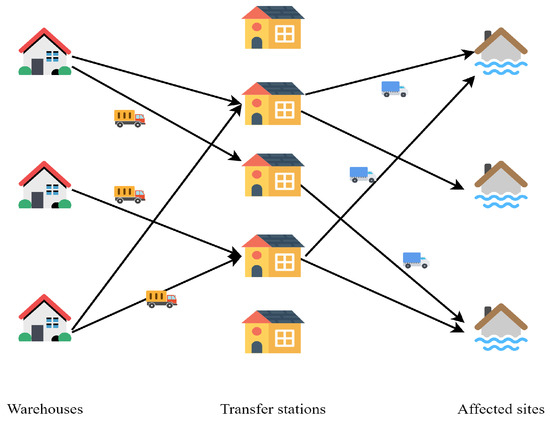
Figure 1. Diagram for emergency materials distribution.

Reinforcement learning, especially multi-armed bandit algorithms (in this paper, we call multi-armed bandit algorithms and reinforcement learning algorithms interchangeably), acts as a powerful approach to tackling large-scale and complex stochastic decision-making problems by simulating the interaction between agent and environment [13,14]. By interacting with the external environment and receiving timely feedback, the algorithm learns to take appropriate actions in different scenarios, making it well-suited for solving stochastic problems. In a real disaster scenario, the transportation times and demands for emergency supplies are random. When the emergency authority makes location planning decision, the subsequent emergency supplies transportation times and the demands for supplies at disaster sites in each period are unobservable. Only when supplies arrive at their destinations are the vehicle transportation times known, and only at the end of each period are new demands realized at affected sites. To better characterize the decision making of emergency authority (agent) in a dynamic and uncertain (random parameters generated from probability distribution) environment, we apply multi-armed bandit algorithms to tackle the transfer stations location planning, with the emergency supplies distribution and allocation in an uncertain environment. Three multi-armed bandit algorithms, including our new developed Geometric Greedy algorithm, are implemented to solve the stochastic model.

To demonstrate the practicality of our model and algorithms, we conduct a case study in the Futian District of Shenzhen, simulating transfer station location selection and emergency material scheduling in response to an urban flood disaster. Analysis shows that the developed Geometric Greedy algorithm is proficient in decision-making in a simulated disaster scenario and achieves better overall performances on computational efficiency and convergence stability compared with the $ϵ$-Greedy algorithm and Upper-Confidence-Bound (UCB) algorithm. We summarize the contributions of this paper as follows:

(1) We design a three-layer emergency logistics network to manage the flow of disaster relief materials and develop a bi-objective, multi-period stochastic integer programming model to support post-disaster decision-making under uncertainty. The model addresses key questions, including which transfer stations should be selected and how many emergency supplies should be transported from warehouses to transfer stations and then to affected sites.

(2) We apply multi-armed bandit approaches in an innovative way to solve the transfer station location planning problem, taking into account the subsequent distribution and allocation of emergency materials under uncertainty. The advantage of using multi-armed bandit algorithms over traditional optimization methods is that they enable the decision-maker to interact with the uncertain environment, allowing for the adjustment of location strategies based on the evolving distribution and allocation of relief supplies in each training episode.

(3) We propose a novel multi-armed bandit (reinforcement learning) algorithm called the Geometric Greedy algorithm, which outperforms the traditional $ϵ$-Greedy algorithm and the Upper Confidence Bound (UCB) algorithm in both computational efficiency and convergence stability.

The paper is organized as follows: Section 2 provides a brief review of related research. Section 3 presents our methodology, which includes a distribution–location–allocation model and three multi-armed bandit algorithms for solving the model. A case study and numerical results are presented in Section 4. Finally, conclusions are drawn in Section 5.

2. Literature Review

Given that our research problem focuses on applying multi-armed bandit algorithms for location planning, along with subsequent dynamic distribution and the allocation of emergency supplies in an uncertain environment, the literature review in this paper is organized into two main streams. The first part addresses literature that jointly tackles facility location and emergency resource distribution problems, as presented in Section 2.1. The second stream discusses the applications of multi-armed bandit approaches—more broadly, reinforcement learning algorithms—in solving emergency management problems, as shown in Section 2.2.

2.1. The Combination Problem of Facility Location and Emergency Resources Distribution

After the sudden outbreak of natural disasters, the appropriate location selection of emergency facilities and efficient delivery of emergency resources to affected areas play a significant role in reducing disaster damages and the survival of disaster victims [15].

In terms of making location and emergency materials distribution decisions under uncertainty, there are a variety of papers addressing this issue by constructing stochastic models. Chang et al. designed a decision-making tool for the government to plan for flood emergency logistics [16]. Two stochastic optimization models were constructed to satisfy the rescue demands at flooding points by properly determining the setup of rescue bases and distributing the engine pumps according to the urgency at each flooding site. Mete and Zabinsky proposed a two-stage stochastic programming model to determine the opening up of medical supply warehouses and the transportation amount of medical supplies from each warehouse to each hospital under different disaster scenarios [17]. Following that was a vehicle routing model, which optimized a series of predetermined routes to make transportation plans. It made a forward step in the emergency response in an uncertain environment by developing a system combining facility location, emergency materials distribution, and emergency vehicle routing in the aftermath of disasters. Ahmadi et al. built a two-stage relief chain to help emergency authorities make decisions under uncertainty [18]. The first stage decision involved the location selection of the distribution centers and the routing strategies from distribution centers to aggregate, and the second stage decision considered the location determination of local depots and the delivery plan from selected depots to traffic analysis zones. Since the damage of the disaster to the road network made the travel time unpredictable, they developed a stochastic multi-depot logistics model under the influence of network failure, involving the minimization of unsatisfied demand, which ensured that adequate emergency materials were transported to the disaster sites. Paul and Zhang developed a two-stage stochastic programming model to make location and transportation planning in the disaster preparedness phase in case of potential hurricane weather [19]. Decision-makers’ risk attitudes were introduced to adjust the number of Points of Distribution selected, and uncertain parameters are characterized by probability distributions rather than a robust adaptive optimization approach to reduce computational complexity. Mohammadi et al. built a humanitarian relief chain by designing a multi-objective fuzzy-based optimization model to make a series of emergency response decisions, including the location selection of the distribution center, and the number of emergency materials distributed [20]. Due to the uncertain nature of the disaster environment, the estimation of model parameters had a large impact on the schedule plan of emergency materials. In this paper, a neutrosophic fuzzy-based approach was employed to handle the uncertainty in the objective functions, which then was further combined with constraints processed by robust optimization to obtain the final model.

Since the emergency materials demand at disaster sites are time-varying, the dynamic distribution of emergency materials is essential to the success of emergency response. Tzeng et al. established an emergency materials distribution system, including the selection of transfer depots, the dynamic emergency materials distribution from upstream (emergency materials collection sites) to midstream (selected transfer depots), and from midstream to downstream (demand points), which set a good example for the construction of a three-layer emergency logistics network [11]. Three objectives considering delivery efficiency and distribution fairness were designed to ensure that every demand point is well satisfied in each time period. Cao et al. regarded sustainability, measured by injury satisfaction, as a significant issue when determining the strategies for distributing emergency materials dynamically [21]. Two objectives were developed to guide the resource allocation process: one was maximizing the lowest injuries’ satisfaction, and another was related to satisfaction variance. This paper highlighted the importance of considering the victims’ feelings in the design of distributing emergency materials. In reaction to the demand-supply incongruence in post-disaster logistics operations, Zhan et al. developed a sequential decision-making framework to tackle the location and emergency materials assignment problem [22]. The established framework answered two important questions: how to ensure the estimation accuracy of demand prediction and how to deliver emergency materials to affected sites in an effective manner. Another research highlight that made this paper distinctive was that the dynamics of the delivery decision were concerned with “deliver now or later” rather than “deliver now or not”.

Besides, there are some papers that considered location selection and dynamic emergency materials distribution in an uncertain environment, which increases the difficulty of the problem. Moreno et al. made contributions to distribution logistics in uncertain disaster situations, characterized by a discrete probability distribution, by considering the location of emergency materials stations and transportation of emergency supplies in each time period [23]. Every time period is further divided into several micro time periods to characterize the flow of commodities more precisely. Compared with existing literature, the deprivation costs [24] were incorporated into the design of objective functions. Numerical results showed that the proposed method could result in the fast delivery of emergency materials and contribute to a fairer distribution. A multi-stage stochastic programming model was proposed by [25] to provide guidance for emergency authorities to deliver emergency materials to disaster points. The state of the road network was taken into consideration, with its capacity both uncertain and dynamic. In addition, an emergency materials transshipment network was constructed involving location, vehicle delivery, and supply distribution decisions.

To date, no literature has applied reinforcement learning algorithms—specifically, multi-armed bandit algorithms—to location planning with dynamic allocation of emergency materials under uncertainty. Our research aims to fill this gap by developing multi-armed bandit algorithms for the location planning of transfer stations, taking into account multi-stage upstream distribution of emergency materials and downstream allocation in a stochastic environment.

2.2. Reinforcement Learning for Emergency Management Problem

As a branch of machine learning, reinforcement learning is concerned with how the agent learns from the interaction with the environment. More specifically, the agents need to adjust their strategies dynamically according to the environment’s feedback to maximize their action rewards or minimize their action costs. Hence, reinforcement learning has flexibility when dealing with randomness from the environment [13,14,26].

There are also several papers concentrating on applying reinforcement learning to emergency path selection, evacuation, rescue operations, and resource allocation. Su et al. applied Q-learning to rescue path selection in times of disasters [27]. In this paper, the rescue team was regarded as the agent, and the path planning model can be taken as a Markov decision process. In response to a dynamic and dangerous environment, numerical experiments showed that the solutions proposed by Q-learning are more reliable, which demonstrated the excellent performance and practical use of reinforcement learning in disaster management. Sarabakha and Kayacan focused on the generation of evacuation plans in buildings when disasters suddenly broke out [28]. A stochastic Q-learning algorithm was proposed in this paper to help create the shortest paths that can lead to the exits of buildings in a three-dimensional space, relieving the pressure of evacuation in an emergency. Nadi and Edrisi built a multi-agent system as a Markov decision process to assist the emergency materials aid and rescue operations [29]. They designed a reinforcement learning approach as the solution procedure for the coordinated system. Results in this paper show that the employment of the model can significantly improve the efficiency of rescue operations. Yan et al. developed a novel rescue dispatch system called MobiRescue to satisfy the number of rescue requests as much as possible, which can overcome the shortcoming that traditional rescue team dispatching approaches are inefficient in the estimation of rescue request positions [30]. The support vector machine method was employed to estimate the distribution of potential rescue calls, and a reinforcement learning approach was devised to improve the rescue efficiency based on the predicted distribution, which had superior performance compared with other methods in the numerical experiments.

Yu et al. did pioneer work on attempting to investigate the applicability of reinforcement learning on a multi-period humanitarian resource allocation problem with deterministic demand [31]. With efficiency, effectiveness, and fairness taken into account in the design of reward functions, the developed $ϵ$-greedy algorithm obtained a tradeoff between exploration and exploitation, which achieved more satisfactory performances compared with existing approaches. Hachiya et al. proposed a model for transporting emergency materials by multiple UAVs (agents) using a Q-learning reinforcement learning algorithm [32]. They showed that it had better performance than meta-heuristics methods in the previous studies and a more stable supply of emergency relief supplies.

Although some studies have attempted to apply reinforcement learning to disaster management problems, the use of these approaches to support disaster response remains limited. Moreover, no existing literature applies reinforcement learning to facility location selection while accounting for the subsequent dynamic distribution and allocation of emergency materials in an uncertain environment. Our research aims to address this gap.

Unlike previous studies, where algorithmic exploration focused primarily on supply allocation, our algorithms emphasize exploration and exploitation in the selection of transfer station locations, while also accounting for upstream emergency materials distribution and downstream allocation in an uncertain environment. When the decision-maker initially plans the locations, the exact transportation times for relief supplies and the precise demands at affected sites for each period are unknown. As a result, the cost (or reward) associated with selecting a particular location plan is inherently random. By applying multi-armed bandit algorithms to the selection of transfer stations, a potential location plan is chosen in each training episode based on specified rules. The decision-maker then distributes and allocates supplies according to estimated transportation times and demands, which are continuously updated with new data gathered during each episode. These updates improve the accuracy of estimations for the next training episode. Ultimately, the multi-armed bandit algorithms guide the selection of the optimal location plan for transfer stations and the corresponding transportation amounts. Our research expands the application of reinforcement learning in the emergency response phase, demonstrating high adaptability to real disaster scenarios.

3. Methodology

In the methodology section, we first present our operational model, followed by our multi-armed bandit (reinforcement learning) algorithms.

3.1. Distribution–Location–Allocation Model

In this section, a bi-objective multi-period stochastic integer programming model is formulated to solve an emergency location, allocation, and distribution problem in an uncertain environment. To reflect real-world constraints, the model excludes scenarios where warehouses send excessive supplies to transfer stations at the outset to meet all future demands in advance since the capacities of transfer stations are limited in reality.

3.1.1. Notations and Definitions

Notations used in the model and algorithms are described below.

Sets and indices
I	set of warehouses.
L	set of candidate transfer stations.
J	set of disaster sites for disaster response.
K	set of emergency materials.
$\xi$	the severity of the disaster.
Parameters
$t_0$	initial time of emergency operations.
T	termination time of emergency operations.
$f_l$	opening cost of transfer station l.
$\gamma$	number of transfer stations selected.
$\eta$	minimum satisfaction rate of emergency materials at disaster sites.
v	average travel speed on the road network.
$d_{il},d_{lj}$	shortest distance from warehouse i to transfer station l, from transfer station l to disaster point j on the road network.
$e_{il},e_{lj}$	unit transportation cost from warehouse i to station l and from station l to disaster point j per hour per unit.
$c_{il},c_{lj}$	transportation time from warehouse i to station l and from station l to disaster site j under the normal traffic condition.
${\omega }_1,{\omega }_2$	weights of the first and the second objective functions.
$Q_i^k$	the initial inventory level of supplies k in warehouse i.
Variables
$q_i^k\left(t\right)$	the amount of supplies k available in warehouse i at the beginning of period t.
$q_l^k\left(t\right)$	the amount of supplies k available in station l at the beginning of period t.
$D_j^k\left(t\right)$	newly generated demand of supplies k at disaster point j at the beginning of period t.
$S_j^k\left(t\right)$	the unsatisfied demand of disaster point j with regard to supplies k at the end of period t.
${\beta }_j\left(t\right)$	penalty parameter for unfulfilled demand at disaster site j in period t.
Decision variables:
$z_l$	whether the candidate station l is chosen to open or not, with 1 indicating it was selected, and 0 otherwise.
$m_{il}^k\left(t\right)$	amount of supplies k transported from warehouse i to station l in period t.
$m_{lj}^k\left(t\right)$	amount of supplies k transported from station l to disaster point j in period t.

3.1.2. Model Formulation

In real disasters, transportation times from supply sites to affected areas may be significantly impacted by damaged road networks, which depend on the disaster’s severity [18]. The devastating effects on the road network can even double transportation times from warehouses to disaster sites [31]. To represent the severity of natural disasters, we assume that the disaster random variable $\xi$ follows a uniform distribution on $[1,2]$, capturing the extent of the damage. We make this assumption for simplicity in characterizing disaster severity, a practice also adopted in the literature [31].

Under disaster uncertainty, transportation times $c_{il}$ are scaled by the disaster extent $\xi$. As a result, the travel times become $\xi c_{il}$ from warehouse i to transfer station l and $\xi c_{lj}$ from station l to affected site j. The penalty for unmet demand reflects the potential economic loss when emergency supply demands are not fully satisfied. Similarly, we model the effect of disaster severity on unmet demand penalties using $\xi {\beta }_j\left(t\right)$. As the severity of the disaster increases, each additional unit of unmet demand results in greater potential losses.

In terms of the objectives the decision-maker wants to achieve, we set the following:

Objective 1: Minimize the opening costs of transfer stations and the transportation costs:

$$F_1=\sum _{l\in L}{f}_l{z}_l+\mathbb{E}\left[\sum _{t=t_0}^T\sum _{k\in K}\left(\sum _{i\in I}\sum _{l\in L}\xi c_{il}{e}_{il}{m}_{il}^k\left(t\right)+\sum _{l\in L}\sum _{j\in J}\xi c_{lj}{e}_{lj}{m}_{lj}^k\left(t\right)\right)\right]$$

Objective 2: Minimize the penalized unsatisfied demand:

$$F_2=\mathbb{E}\left[\sum _{t=t_0+1}^T\sum _{j\in J}\sum _{k\in K}\xi {\beta }_j\left(t\right)S_j^k\left(t\right)\right]$$

The above objectives are commonly seen in literature that concerns facility location and emergency resource allocation [11]. The decision-maker’s optimization problem is formulated as below.

$$\begin{array}{c}{H}^{*}\left(t_0\right)=\underset{z,m}{min}H(z,t_0,m)=\underset{z,m}{min}({\omega }_1{F}_1+{\omega }_2{F}_2)\hfill \\ \mathrm{s}.\mathrm{t}.\hfill \end{array}$$

(Prob1)

$$S_j^k\left(t\right)=S_j^k(t-1)-\sum _{l\in L}{m}_{lj}^k\left(t\right)+D_j^k\left(t\right)\hspace{1em}\forall j\in J,k\in K,t=t_0+1,\dots ,T$$

(1)

$$\sum _{l\in L}{m}_{lj}^k\left(t\right)\le S_j^k(t-1)+D_j^k\left(t\right)\hspace{1em}\forall j\in J,k\in K,t=t_0+1,\dots ,T$$

(2)

$$\mathbb{P}\left(\eta \left(S_j^k(t-1)+D_j^k\left(t\right)\right)\le \sum _{l\in L}{m}_{lj}^k\left(t\right)\right)\ge \alpha \hspace{1em}\forall j\in J,k\in K,t=t_0+1,\dots ,T$$

(3)

$$\sum _{l\in L}{m}_{il}^k\left(t\right)\le q_i^k\left(t\right)\hspace{1em}\forall i\in I,k\in K,t=t_0,t_0+1,\dots ,T$$

(4)

$$\sum _{j\in J}{m}_{lj}^k\left(t\right)\le q_l^k\left(t\right)z_l\hspace{1em}\forall l\in L,k\in K,t=t_0,t_0+1,\dots ,T$$

(5)

$$q_l^k\left(t_0\right)=0\hspace{1em}\forall l\in L,k\in K$$

(6)

$$q_l^k\left(t\right)=q_l^k(t-1)+\sum _{i\in I}{m}_{il}^k(t-1)-\sum _{j\in J}{m}_{lj}^k(t-1)\hspace{1em}\forall l\in L,k\in K,t=t_0+1,\dots ,T$$

(7)

$$q_i^k\left(t_0\right)=Q_i^k\hspace{1em}\forall i\in I,k\in K$$

(8)

$$q_i^k\left(t\right)=q_i^k(t-1)-\sum _{l\in L}{m}_{il}^k(t-1)\hspace{1em}\forall i\in I,k\in K,t=t_0+1,\dots ,T$$

(9)

$$\sum _{l\in L}{z}_l=\gamma$$

(10)

$$S_j^k\left(t_0\right)=0,\hspace{1em}\forall j\in J,k\in K$$

(11)

$$S_j^k\left(t\right)\in \mathbb{Z},\hspace{1em}\forall j\in J,k\in K,t=t_0+1,\dots ,T$$

(12)

$$m_{lj}^k\left(t\right),m_{il}^k\left(t\right)\in \mathbb{N}\hspace{1em}\forall i\in I,j\in J,k\in K,t=t_0,t_0+1,\dots ,T$$

(13)

$$z_l\in \{0,1\},\hspace{1em}\forall l\in L$$

(14)

The objective function aims to minimize the weighted sum of two objectives: opening costs, expected transportation costs and expected penalized unsatisfied demand. Constraint (1) models how the unsatisfied demand at each disaster site evolves over time. Specifically, the unsatisfied demand at site j at the end of period t equals the unsatisfied demand at the end of period $t-1$ plus newly generated demand, minus the emergency materials received in period t. Constraint (2) ensures that the emergency materials delivered from transfer stations to affected sites do not exceed the unsatisfied demand, avoiding the waste of supplies. Constraint (3) is a chance constraint, ensuring that the probability of satisfying at least $\eta$ of the demand at each site in each period is maintained at a confidence level $\alpha$. This can also be viewed as a fairness constraint, as it ensures that the needs of every disaster site are addressed equitably. Constraint (4) ensures that the total emergency materials transported to transfer stations do not exceed the available stock at each warehouse during each period. Constraint (5) guarantees that the materials dispatched from a transfer station remain within its inventory capacity if the station is operational; otherwise, no stock will be allocated to that station.

Constraint (6) sets the initial inventory level at each transfer station to 0. Constraint (7) defines the flow of inventory at each transfer station: the current stock equals the previous period’s inventory plus replenishments from warehouses, minus materials sent to local disaster sites. Similarly, constraint (8) establishes the initial inventory level at each warehouse, while constraint (9) models the stock flow at each warehouse. Specifically, the inventory at warehouse i in the current period equals the previous inventory minus the materials transferred to the selected transfer stations. Constraint (10) limits the total number of transfer stations to $\gamma$, controlling costs and minimizing the waste of emergency resources. Constraints (11) and (12) initialize the unsatisfied demand at affected sites at $t_0$ to 0. Additionally, all variables related to quantities must be integers, as required. Constraint (13) ensures that the quantities of emergency materials transferred between the three layers are natural numbers. Finally, constraint (14) governs the selection of transfer stations. If a candidate station is selected, the corresponding variable is set to 1; otherwise, it remains 0.

In the developed bi-objective multi-period stochastic integer programming model, there are three emergency decisions that must be made sequentially: the selection of transfer station locations, the distribution of upstream emergency materials, and the allocation of downstream emergency materials. A timeline is provided below (see Figure 2) to illustrate the series of actions in each time period.

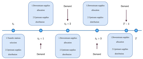
Figure 2. Timeline for the emergency logistics operations.

3.1.3. Timeline for the Emergency Operations

The locations of transfer stations must be determined at the beginning of the first period $t_0$; following this, the decision on upstream emergency materials distribution is made, which involves distributing emergency materials from warehouses to transfer stations. The first-stage decision does not include the allocation of supplies from selected transfer stations to disaster sites, as the delivery from warehouses to transfer stations occupies the first period, and there is no inventory in the temporarily opened transfer stations during this stage (in this paper, we call stage and period interchangeably).

After the locations of transfer stations are established and emergency materials are transported from warehouses to these stations, the downstream supplies allocation and upstream emergency materials distribution decisions are made sequentially in the subsequent stages. It is important to note that the downstream allocation decision always precedes the upstream distribution decision at each stage, as the delivery of emergency materials is demand-oriented. The amount transported from warehouses to transfer stations depends on the inventory levels at each transfer station, which are closely linked to the allocation amounts from transfer stations to disaster sites. Additionally, emergency material demands are generated starting from the beginning of period $t_0+1$ and continue until the beginning of period $T-1$. As a result, unsatisfied demands may persist from period $t_0+1$ onward.

3.2. Multi-Armed Bandit (Reinforcement Learning) Algorithms

3.2.1. Geometric Greedy Algorithm

As noted by [16], evaluating the expectation in the objective function poses a significant challenge when solving a stochastic programming model. Most traditional approaches to addressing stochastic discrete optimization problems focus on internal or external sampling-based approximation methods. For instance, sample average approximation (SAA) aims to estimate the true objective of the stochastic problem by averaging over a large generated sample, effectively transforming the stochastic problem solution into the average of solutions for a series of deterministic problems [12]. Sampling methods typically generate numerous samples at the outset and then search for the optimal solution within a feasible region. This approach results in a fixed emergency materials allocation amount, which cannot adapt to evolving disaster scenarios with new data.

In contrast, reinforcement learning dynamically adjusts action strategies in each training episode within an uncertain environment. Consequently, the selected transfer station locations and computed transportation amounts may vary from one training episode to the next as new information becomes available.

In this paper, we develop a novel multi-armed bandit algorithm, termed the Geometric Greedy algorithm, to address the bi-objective multi-period stochastic integer programming model. In addition to the notations defined previously, we introduce several auxiliary variables and estimators that will be utilized in the subsequent algorithm description.

Auxiliary Variables
${\mathbb{L}}_r$	transfer stations combination.
$m_{ilj}^k\left(t\right)$	amount of supplies k transported from warehouse i to station l in period t and
	planned to be transported to disaster point j in period $t+1$.
$q_{il}^k\left(t\right)$	stocks of supplies k at station l in period t received from warehouse i.
${\Delta }_{ilj}^k\left(t\right)$	discriminants that determine transportation amount.
${\eta }_{ilj}^k\left(t\right)$	percentage bounds for transportation amount.
$n_l$	selection times of station l in the algorithm.
$N_r$	selection times of station combination ${\mathbb{L}}_r$ in the algorithm.

Estimators in the stochastic model
${\widehat{\beta }}_j\left(t\right)$	estimator of $\mathbb{E}\left(\xi \right){\beta }_j\left(t\right)$.
${\widehat{D}}_j\left(t\right)$	estimator of $\mathbb{E}\left(D_j\left(t\right)\right)$.
${\widehat{c}}_{il}$	estimator of $\mathbb{E}\left(\xi \right)c_{il}$.
${\widehat{c}}_{lj}$	estimator of $\mathbb{E}\left(\xi \right)c_{lj}$.
$\widehat{H}\left(r\right)$	estimator of the weighted cost H with station combination ${\mathbb{L}}_r$.
${\widehat{\Delta }}_{ilj}^k\left(t\right)$	estimator of $\mathbb{E}\left(\xi \right){\Delta }_{ilj}^k\left(t\right)$.

Agent and Action Set

In this paper, the decision-maker in the emergency department acts as the learning agent responsible for making three critical decisions: transfer station selection, upstream emergency materials distribution, and downstream emergency materials allocation. The learning agent executes actions $m_{lj}^k\left(t\right)$, $m_{il}^k\left(t\right)$, and $z_l$. Among these decisions, the exploration–exploitation aspect of the algorithm focuses on the location planning of transfer stations $z_l$.

Environment

In this paper, the environment comprises warehouses, candidate transfer stations, and affected sites. The learning agent interacts with this environment by taking actions based on estimations of random transportation times and penalized unsatisfied demand. The emergency materials stocks in the warehouses and transfer stations are also influenced by the decisions made by the agent.

Cost/Reward Function

The objective function $H^{*}\left(t_0\right)$ proposed in this study aims to minimize the weighted costs associated with opening transfer stations, transporting emergency materials, and penalizing unsatisfied demand. And since the algorithm’s exploration–exploitation part emphasizes the location planning of transfer stations $z_l$ (a one-step decision in each training episode), the agent’s cost function (Q-function) can be taken as the objective $H^{*}\left(t_0\right)$ for simplicity.

Core Concept of Geometric Greedy Algorithm

Our Geometric Greedy algorithm explores combinations of stations using a geometric distribution, where the parameter p controls the exploration level. Based on what the algorithm has learned in previous episodes, it selects the station combination resulting in the least total cost with probability p, the combination resulting in the second least total cost with probability $p(1-p)$, the combination resulting in the third least total cost with probability $p{(1-p)}^2$, and so forth. The optimal transportation amount is determined by defined “discriminants”, which will be discussed later. The signs of these discriminants indicate how much supply should be transferred from one station to another in each period.

Materials distribution and allocation decisions can ultimately be made using updating estimators in each episode, with the estimators of the defined discriminants playing a key role in supply transportation. The schematic diagram for the proposed Geometric Greedy algorithm is shown in Figure 3.

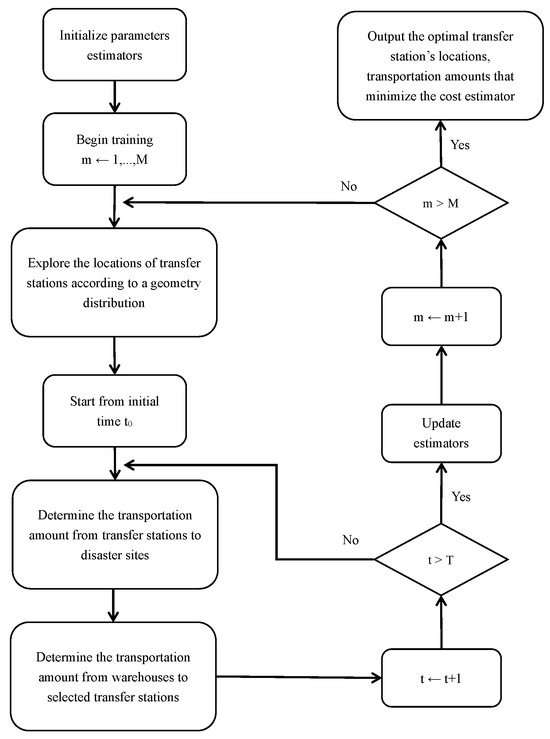
Figure 3. Schematic diagram of Geometric Greedy algorithm.

The original problem (Prob1) can be transformed into an equivalent form, as presented in the theorem below, from which the new concept of “discriminants” naturally emerges. By minimizing this equivalent cost function, the discriminants can effectively determine the transportation amounts.

Theorem 1.

Let $m_{ilj}^k\left(t\right)$ be the amount of supplies k transported from warehouse i to station l in period t and planned to be transported to disaster point j in period $t+1$. Let

$${\Delta }_{ilj}^k\left(t\right):={\omega }_1{c}_{il}{e}_{il}+{\omega }_1{c}_{lj}{e}_{lj}-{\omega }_2\sum _{s=t+1}^T{\beta }_j\left(s\right),\hspace{1em}t=t_0,t_0+1,\dots ,T,$$

and these Δ’s are named “discriminants”. Then the following optimization problem (Prob2) is equivalent to (Prob1) subject to the common constraints (1)–(14).

$${\tilde{H}}^{*}\left(t_0\right)=\underset{z,m}{min}\mathbb{E}\left({\omega }_1\sum _l{f}_l{z}_l+\sum _{t=t_0}^T\sum _{i,l,j,k}\xi {\Delta }_{ilj}^k\left(t\right)m_{ilj}^k\left(t\right)\right).$$

(Prob2)

The proof of the theorem can be found in the Appendix A. If the location decision $z_l$ is fixed, then by Theorem 1 it suffices to minimize $\sum {\Delta }_{ilj}^k\left(t\right)m_{ilj}^k\left(t\right)$. Therefore, we need to set $m_{ilj}^k\left(t\right)$ to be as large as possible when ${\Delta }_{ilj}^k\left(t\right)\le 0$ and to set $m_{ilj}^k\left(t\right)$ to be as small as possible when ${\Delta }_{ilj}^k\left(t\right)>0$.

In addition to the objective function, addressing the chance constraint (3) is essential for solving the model. The theorem below is proposed to tackle this issue. Since each disaster point generates new demand randomly, we need to prepare additional supplies at transfer stations in advance. However, we must also avoid over-preparing supplies, as this would lead to increased transportation costs. The key idea is to closely examine the Poisson distribution.

Theorem 2.

For $D_j^k\left(t\right)\sim \mathrm{Poisson}\left({\lambda }_j^k\left(t\right)\right)$, if ${\lambda }_j^k\left(t\right)\ge 1$ and if $\delta \ge 2{(-{\lambda }_j^k\left(t\right)ln(1-\alpha ))}^{1/2}$, then

$$\mathbb{P}(D_j^k\left(t\right)>{\lambda }_j^k\left(t\right)+\delta )\le 1-\alpha .$$

The proof of the theorem can be found in the Appendix A. Specifically, to satisfy the chance constraint (3), we need to prepare additional supplies k of at least $2{(-{\lambda }_j^k\left(t\right)ln(1-\alpha ))}^{1/2}$ than the mean value of newly generated demand for each disaster point j in period t at transfer stations. In this case, new demands of disaster points may still not be satisfied, but this happens only with a small probability $1-\alpha$.

Description of the Geometric Greedy Algorithm

The detailed procedures of the Geometric Greedy algorithm are as follows. Readers can also follow the algorithm pseudo code provided in Appendix B.

Step 1: We set the number of training episodes to be M and put all possible transfer station selection combinations into a set named $\left\{{\mathbb{L}}_r\right\}$. The counting variables, $n_l$ and $N_r$, are introduced to record the number of times that a single station l and a transfer station combination ${\mathbb{L}}_r$ are selected, respectively, in the previous training episodes. More specifically, if the selected location combination ${\mathbb{L}}_r$ contains transfer station l in one training episode, both the counts of $n_l$ and $N_r$ will be incremented by 1. Moreover, the estimators for random parameters and cost function (objective function), ${\widehat{\beta }}_j\left(t\right),{\widehat{D}}_j^k\left(t\right),{\widehat{c}}_{il},{\widehat{c}}_{lj}$, and $\widehat{H}\left(r\right)$, are initialized to be 0 for each $i\in I,l\in L,j\in J,k\in K,t=t_0+1,\dots ,T$. Given a training episode m, implement Step 2–Step 10.

Step 2: We initialize the amount $q_i^k\left(t_0\right)$, supplies k available in warehouse i in the beginning of period $t_0$, to be $Q_i^k$ (Constraint (8)), and the amount $q_{il}^k\left(t_0\right)$ of supplies k stocked at station l received from warehouse i in the beginning of period $t_0$ to be 0. The variable unsatisfied demand $S_j^k\left(t_0\right)$ is also initialized to 0 in the beginning (Constraint (11)). After that, we generate a severity variable $\xi$ from $\mathrm{Uniform} [1,2]$ and a positive integer o from $1+G\left(p\right)$, where $G\left(p\right)$ denotes the Geometry distribution with parameter p. Then we select the station combination ${\mathbb{L}}_r$ such that $\widehat{H}\left(r\right)$ is the o-th least. In other words, we choose stations combination ${\mathbb{L}}_r$ such that $\widehat{H}\left(r\right)$ is the o-th least with probability $p{(1-p)}^{o-1}$. After the combination ${\mathbb{L}}_r$ is chosen, the counts of $N_r$ and the recording variable $n_l$ of each transfer station contained in the combination will be incremented by 1. Correspondingly, the weighted opening-up cost ${\omega }_1{\sum }_{l\in {\mathbb{L}}_r}{f}_l$ is computed and assigned to the cost function H.

Step 3: By the definition of the discriminants in Theorem 1, we calculate the estimators ${\widehat{\Delta }}_{ilj}^k\left(t\right)$ of discriminants as functions of transportation time estimators ${\widehat{c}}_{il},{\widehat{c}}_{lj}$ and of penalty estimators ${\widehat{\beta }}_j\left(t\right)$:

$${\widehat{\Delta }}_{ilj}^k\left(t\right):={\omega }_1{\widehat{c}}_{il}{e}_{il}+{\omega }_1{\widehat{c}}_{lj}{e}_{lj}-{\omega }_2\sum _{s=t+1}^T{\widehat{\beta }}_j\left(s\right),\hspace{1em}i\in I,l\in {\mathbb{L}}_r,j\in J,k\in K,t=t_0,\dots ,T.$$

We also define $m_{ilj}^k\left(t\right)$ as the amount of supplies k transported from warehouse i to station l in period t and prepared to transport to disaster site j in period $t+1$. In Theorem 1, we prove the equivalence of optimization problem (Prob1) and problem (Prob2) which regards $z_l,m_{ilj}^k\left(t\right)$, and we find that $m_{ilj}^k\left(t\right)$ should be as large as possible if ${\widehat{\Delta }}_{ilj}^k\left(t\right)\le 0$ and as small as possible if ${\widehat{\Delta }}_{ilj}^k\left(t\right)>0$. In addition, considering the constraint (2) and constraint (3), the largest $m_{ilj}^k\left(t\right)$ cannot surpass $S_j^k\left(t\right)+D_j^k(t+1)$, and the smallest $m_{ilj}^k\left(t\right)$ must ensure equity, i.e.,

$$\sum _{i,l}{m}_{ilj}^k\left(t\right)\le S_j^k\left(t\right)+D_j^k(t+1)\hspace{1em}\mathrm{and}\hspace{1em}\mathbb{P}\left(\eta \left(S_j^k\left(t\right)+D_j^k(t+1)\right)\le \sum _{i,l}{m}_{ilj}^k\left(t\right)\right)\ge \alpha .$$

Thus, we can set percentage ${\eta }_{ilj}^k\left(t\right)$ to adjust the transportation amount $m_{ilj}^k\left(t\right)$:

$${\eta }_{ilj}^k\left(t\right)=\left\{\begin{array}{cc}1,\hfill & \mathrm{if}{\widehat{\Delta }}_{ilj}^k\left(t\right)\le 0;\hfill \\ \eta ,\hfill & \mathrm{if}{\widehat{\Delta }}_{ilj}^k\left(t\right)>0.\hfill \end{array}\right.\hspace{1em}i\in I,l\in {\mathbb{L}}_r,j\in J,k\in K,t=t_0,\dots ,T-1.$$

If ${\eta }_{ilj}^k\left(t\right)=1$, we can set $m_{ilj}^k\left(t\right)$ to be larger to fulfill $S_j^k\left(t\right)+D_j^k(t+1)$ to the best; or if ${\eta }_{ilj}^k\left(t\right)=\eta$, then we will not set $m_{ilj}^k\left(t\right)$ to be larger once $\eta (S_j^k\left(t\right)+D_j^k(t+1))$ can be fulfilled. In other words, ${\eta }_{ilj}^k\left(t\right)$ sets an upper bound and a low bound to control the transportation amount of emergency materials. Then, given period t from $t_0$ to T, implement Step 4–Step 9.

Step 4: Initialize $m_{il}^k\left(t\right)$, $m_{lj}^k\left(t\right)$, and $m_{ilj}^k\left(t\right)$ to 0, where $m_{il}^k\left(t\right)$ and $m_{lj}^k\left(t\right)$ are the amount of supplies k transported from warehouse i to station l and from station l to disaster point j in period t, and $m_{ilj}^k\left(t\right)$ is the amount of supplies k transported from warehouse i to station l in period t and then prepared to transport to disaster point j in period $t+1$. New demands then arise at disaster points, namely $S_j^k\left(t\right)\leftarrow S_j^k(t-1)+D_j^k\left(t\right)$.

Step 4 aims to send supplies from stations to disaster points to ensure at least $\eta$ percentage of the unsatisfied demand at each disaster site is satisfied, and update the estimator ${\widehat{D}}_j^k\left(t\right)$. We sort ${\widehat{\Delta }}_{ilj}^k\left(t\right)$ in an increasing order with respect to $i\in I$, $l\in {\mathbb{L}}_r$, $j\in J$ to prioritize allocation order and amount according to the demand urgency at disaster sites. In this order of $i,l,j$, we increase $m_{lj}^k\left(t\right)$ by $min(\eta S_j^k\left(t\right)-{\sum }_{l\in {\mathbb{L}}_r}{m}_{lj}^k\left(t\right),q_{il}^k\left(t\right))$ and decrease $q_{il}^k\left(t\right)$ by the same amount. The amount $\eta S_j^k\left(t\right)$ is the minimum that disaster point j must be satisfied. The difference $\eta S_j^k\left(t\right)-{\sum }_{l\in {\mathbb{L}}_r}{m}_{lj}^k\left(t\right)$ tells us how much remains to fulfill $\eta$ of the unsatisfied demand $S_j^k\left(t\right)$ at the current period. The amount $q_{il}^k\left(t\right)$ is the amount of supplies k stored at station l in period t that was received from warehouse i. Taking a minimum ensures that the transportation amount is no larger than the inventory at station l received from warehouse i. The update mechanism of estimator ${\widehat{D}}_j^k\left(t\right)$ is based on the average of the values in the previous episodes. Namely, ${\widehat{D}}_j^k\left(t\right)\leftarrow {\displaystyle \frac{(m-1){\widehat{D}}_j^k\left(t\right)+D_j^k\left(t\right)}{m}}$.

Step 5: Similarly, in the order of increasing ${\widehat{\Delta }}_{ilj}^k\left(t\right)$, we increase $m_{lj}^k\left(t\right)$ by

$$min\left[max\left({\eta }_{ilj}^k\left(t\right)S_j^k\left(t\right)-\sum _{l\in {\mathbb{L}}_r}{m}_{lj}^k\left(t\right),0\right),q_{il}^k\left(t\right)\right],\hspace{1em}l\in {\mathbb{L}}_r,j\in J,k\in K.$$

and decrease $q_{il}^k\left(t\right)$ by the same amount. Step 5 aims to send disaster points more supplies to reduce the weighted cost after $\eta$ percent of demands have been met. Theorem 1 justifies this procedure. As ${\widehat{\Delta }}_{ilj}^k\left(t\right)$ increases, the percent ${\eta }_{ilj}^k\left(t\right)$ decreases, so taking a maximum with 0 can avoid a negative transportation amount from station l to disaster site j. Based on that, we take a minimum between $max({\eta }_{ilj}^k\left(t\right)S_j^k\left(t\right)-{\sum }_{l\in {\mathbb{L}}_r}{m}_{lj}^k\left(t\right),0)$ and $q_{il}^k\left(t\right)$ to guarantee that the transportation amount is no larger than the inventory stored at station l from warehouse i.

Step 6: After supplies arrive at disaster points, the transportation time $c_{lj}\left(\xi \right)$ from station l to disaster site j is realized. We update the estimators ${\widehat{c}}_{lj}$ using transportation time $c_{lj}\left(\xi \right)$, $l\in {\mathbb{L}}_r,j\in J$, add the transportation cost ${\omega }_1{\sum }_{l,j,k}\xi c_{lj}{e}_{lj}{m}_{lj}^k\left(t\right)$ to H, and obtain the updated unsatisfied demands of disaster points $S_j^k\left(t\right)\leftarrow S_j^k\left(t\right)-{\sum }_{l\in {\mathbb{L}}_r}{m}_{lj}^k\left(t\right)$. The update mechanisms of estimators, including ${\widehat{c}}_{il}$ and ${\widehat{c}}_{lj}$, are based on the average over the values in the previous episodes that select the location l. Namely, ${\widehat{c}}_{lj}\leftarrow {\displaystyle \frac{(n_l-1){\widehat{c}}_{lj}+\xi c_{lj}}{n_l}}$ for $l\in {\mathbb{L}}_r$.

Step 7: This step aims to transfer supplies from warehouses to stations. We sort ${\widehat{\Delta }}_{ilj}^k\left(t\right)$ in an increasing order with respect to $i\in I$, $l\in {\mathbb{L}}_r$, $j\in J$ to prioritize the distribution order and amount according to the demand urgency at disaster points. In this order of $i,l,j$, we increase $m_{ilj}^k\left(t\right)$ by

$$\begin{array}{c}min\left\{max\left[{\eta }_{ilj}^k(t+1)(S_j^k\left(t\right)+{\widehat{D}}_j^k(t+1)+2{(-{\widehat{D}}_j^k(t+1)ln(1-\alpha ))}^{1/2})\right.\right.\hfill \\ \hfill -\left.\left.\sum _{i\in I,l\in {\mathbb{L}}_r}{m}_{ilj}^k\left(t\right),0\right],q_i^k\left(t\right)\right\},\hspace{1em}i\in I,l\in {\mathbb{L}}_r,j\in J,k\in K.\hfill \end{array}$$

and decrease $q_i^k\left(t\right)$ by the same amount. The amount $S_j^k\left(t\right)+{\widehat{D}}_j^k(t+1)$ is a prediction of the unsatisfied demand at disaster point j in the next stage, and the additional term $2{(-{\widehat{D}}_j^k(t+1)ln(1-\alpha ))}^{1/2}$ is necessary due to the chance constraint (3), see also Theorem 2. Taking a maximum with 0 can avoid negative transportation amount from warehouse i to station l. Taking a minimum with $q_i^k\left(t\right)$ guarantees that the transportation amount is no larger than the inventory in warehouse i. Once $m_{ilj}^k\left(t\right)$’s are fixed, we sum them up to obtain $m_{il}^k\left(t\right)\leftarrow {\sum }_{j\in J}{m}_{ilj}^k\left(t\right)$.

Step 8: After supplies arrive at transfer stations, the transportation time $c_{il}\left(\xi \right)$ from warehouse i to station l is realized. we update the estimators ${\widehat{c}}_{il}$ for transportation time $c_{il}\left(\xi \right)$, $i\in I,l\in {\mathbb{L}}_r$, add the transportation cost ${\omega }_1{\sum }_{i,l,k}\xi c_{il}{e}_{il}{m}_{il}^k\left(t\right)$ to H, and update the stocks of supplies at stations $q_{il}^k\left(t\right)\leftarrow q_{il}^k\left(t\right)+m_{il}^k\left(t\right)$.

Step 9: At the end of a period, the true value of ${\beta }_j(\xi ,t)$ is realized, which can be used to update the estimators ${\widehat{\beta }}_j\left(t\right)$. The weighted penalty for unmet demand ${\omega }_2{\sum }_{j,k}\xi {\beta }_j\left(t\right)S_j^k\left(t\right)$, is then added to the cost function H. The update mechanisms of estimator ${\widehat{\beta }}_j\left(t\right)$ is based on the average over the values in the previous episodes. Namely, ${\widehat{\beta }}_j\left(t\right)\leftarrow {\displaystyle \frac{(m-1){\widehat{\beta }}_j\left(t\right)+\xi {\beta }_j\left(t\right)}{m}}$.

Step 10: Repeat Step 4–Step 9 until the final period T, we can obtain the total cost H and update the cost estimator $\widehat{H}\left(r\right)$. The update mechanism of $\widehat{H}\left(r\right)$ is based on the average over the values in the previous episodes that select the same transfer station combination ${\mathbb{L}}_r$. Namely, $\widehat{H}\left(r\right)\leftarrow {\displaystyle \frac{(N_r-1)\widehat{H}\left(r\right)+H}{N_r}}$. Go back to Step 2 to start a new training episode.

3.2.2. $ϵ$-Greedy Algorithm and Upper-Confidence-Bound (UCB) Algorithm

The $ϵ$-Greedy algorithm is one of the most popular multi-armed bandit algorithms and has been widely applied in many areas [26]. The basic principle of the $ϵ$-Greedy algorithm is to balance the tradeoff between exploration and exploitation to minimize the agent’s cost by controlling an exploration parameter $ϵ$. In our problem, the $ϵ$-Greedy algorithm can be implemented by, in each learning episode, choosing such a station combination ${\mathbb{L}}_r$ that $\widehat{H}\left(r\right)$ is the least in the previous learning episodes with probability $1-ϵ$, and choosing any one of other ${\mathbb{L}}_r$’s uniformly with probability $ϵ$. To be more precise, we choose ${\mathbb{L}}_r$ according to

$$r\leftarrow \left\{\begin{array}{cc}arg\underset{r}{min}\widehat{H}\left(r\right)=:r^{*},\hfill & \mathrm{with} \mathrm{probability} 1-ϵ,\hfill \\ r\ne r^{*},\hfill & \mathrm{with} \mathrm{probability} ϵ\hfill \end{array}\right.$$

The Upper-Confidence-Bound (UCB) algorithm is another commonly used multi-armed bandit algorithm [33]. The particularity of the UCB algorithm lies in that the algorithm tends to choose actions that have been tried the least in the previous training episodes. For our problem, in the m-th learning episode, we choose the station combination ${\mathbb{L}}_r$ with the least of the following quantities:

$$\widehat{H}\left(r\right)-\lambda \sqrt{{\displaystyle \frac{lnm}{N_r}}},$$

where $\lambda$ is a suitable confidence parameter that controls the level of exploration. Recall that in our paper, $N_r$ represents the number of times the station combination ${\mathbb{L}}_r$ has been selected up to the m-th training episode. Therefore, if $N_r$ is large for a given location combination ${\mathbb{L}}_r$, the algorithm will select this combination with a lower probability, in accordance with the UCB algorithm’s principle of favoring actions that have been explored less in previous training episodes. Also, if $\lambda$ is large, the exploration intensity would be more significant.

Compared to the $ϵ$-Greedy algorithm, the Geometric Greedy algorithm reduces exploration for higher-cost location plans, enhancing the stability of learning outcomes. Furthermore, by eliminating the confidence correction used in the Upper-Confidence-Bound (UCB) algorithm, the Geometric Greedy algorithm achieves lower computational demands and faster execution times.

4. Case Study

To verify the validity of the models and algorithms, this paper uses an extreme urban flood disaster that occurred in Shenzhen, Guangdong Province, China, as a case study. According to [34], the maximum half-hourly rainfall in Futian District on 11 April 2019, reached 73.4 mm—equivalent to a 100-year rainstorm—and resulted in 11 deaths. The disaster disrupted transportation in several areas, leaving many people trapped [35]. To implement a rapid emergency response, minimize casualties and property losses, and restore normal city operations as soon as possible, the government needed to deliver emergency aid (e.g., medical equipment) promptly to the victims at designated disaster stations. However, due to the dispersed locations of the affected areas, the direct delivery of emergency materials was not feasible. In such situations, a three-layer emergency logistics network can be employed. In this network, large trucks transport emergency supplies from warehouses to transfer stations near disaster sites. From these stations, smaller trucks distribute the materials to the affected locations.

4.1. Data Collection and Preprocessing

According to the data provided by the local emergency department, there are three emergency materials aid warehouses in Futian District. With the data collected from the Shenzhen municipal government data open platform, 11 flood sites required emergency materials following the sudden urban flood outbreak. Additionally, 15 candidate transfer stations, selected from Shenzhen’s natural disaster emergency shelters—including schools, parks, and other facilities—were identified as potential distribution points. The locations of the candidate transfer stations, warehouses, and affected sites on Futian District’s road network are shown in Figure 4.

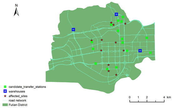
Figure 4. The distribution of candidate transfer stations, warehouses, and affect sites on the road network in Futian District.

4.1.1. Model Parameter Setting

To better simulate the real disaster scenario in Futian District, we refer to relevant historical reports and set $t_0=0$, with the total duration of emergency operations spanning four periods ($T=4$), each lasting one hour. For computational simplicity, we focus on a single type of emergency material ($k=1$): medical boxes. When multiple types of emergency materials need to be delivered and allocated, they can be handled similarly. We set the minimum satisfaction rate $\eta$ and the confidence level $\alpha$ in constraint (4) to 70% and 99%, respectively. Regarding the number of transfer stations to be selected, $\gamma$ is set to 3, considering that only 15 candidate transfer stations are available in Futian District. The opening costs of these 15 candidate stations are provided in Table A1 in the Appendix C. We initially assume that emergency materials are abundant, with the initial stock levels at the three warehouses ($Q_i^k$) set to 500, 900, and 600 units, respectively. For the weights of the two objectives, we assign ${\omega }_1={\omega }_2={\displaystyle \frac{1}{2}}$.

For simplicity, we do not account for differences in the trucks used to transport emergency materials between warehouses, transfer stations, and affected sites. In other words, the trucks used across different layers are treated as identical, with a transportation cost of $5 per hour per unit. This cost is widely adopted by the local emergency department for transporting medical equipment. We define the transportation times $c_{il}$ from warehouse i to transfer station l and from transfer station l to disaster site j under normal traffic conditions (i.e., without disasters) as ${\displaystyle \frac{d_{il}}{v}}$ and ${\displaystyle \frac{d_{lj}}{v}}$, respectively, (see Table A2 and Table A3 in the Appendix C). Here, $d_{il}$ and $d_{lj}$ represent the shortest distances from warehouse i to transfer station l and from transfer station l to disaster site j, respectively, as determined using ArcGIS 10.6. The road network data for Futian District, Shenzhen, was downloaded from OpenStreetMap, and the shortest distances were computed using the Shortest Path Analysis toolbox in ArcMap 10.6. The average travel speed on the road network is assumed to be 30 km/h, a realistic estimate for urban areas.

To simulate the dispatch of emergency materials under urban flood conditions, we assume that the disaster random variable $\xi$, representing the severity of the disaster, follows a uniform distribution on $[1,2]$ to capture the varying degrees of disaster impact. Under disaster uncertainty, the transportation times $c_{il}$ and $c_{lj}$, as well as the penalty parameters ${\beta }_j\left(t\right)$, are scaled by the factor $\xi$. The travel times become $\xi c_{il}$ and $\xi c_{lj}$, reflecting the significant disruption to the road network caused by the disaster, potentially doubling travel times from warehouses to disaster sites [31]. Similarly, the penalty term becomes $\xi {\beta }_j\left(t\right)$ to account for the increased economic loss as disaster severity rises. Details of the penalty values ${\beta }_j\left(t\right)$ can be found in Table A4 in the Appendix C. The demand for emergency materials k at affected site j during period t, denoted as $D_j^k\left(t\right)$, is assumed to follow a Poisson distribution [36] with rate parameter ${\lambda }_j^k\left(t\right)$. These rate parameters ${\lambda }_j^k\left(t\right)$ are also provided in the demand columns of Table A4.

4.1.2. Algorithm Parameter Setting

For each of the proposed three Multi-armed bandit (reinforcement learning) algorithms: $ϵ$-Greedy algorithm, Upper-Confidence-Bound(UCB) algorithm, and the new developed Geometric Greedy algorithm, we conduct 10 numerical experiments, and each experiment contains 20,000 learning episodes. The selections of transfer stations’ locations, averages of objective values in experiments, and algorithm execution times are recorded separately.

The exploration probability $ϵ$ is set to be $0.3$ in the $ϵ$-Greedy algorithm. And the confidence parameter $\lambda$ is set to be 6000 in the UCB algorithm. For the proposed Geometric Greedy algorithm, the geometric factor p is taken as 0.7 to make sure that its exploitation probability for ${\mathbb{L}}_r$ that minimizes $\widehat{H}\left(r\right)$ is the same as the $ϵ$-Greedy algorithm.

4.2. Model Results

The numerical experiments are conducted on a computer system that consists of Intel(R) Core(TM) i7-8650U CPU @ 1.90GHz 2.11GHz and a RAM of 16 GB. All the algorithms are implemented in Wolfram Mathematica 12.0.

Three Multi-Armed Bandit Algorithms

Convergence stability and computational efficiency are two important indicators for evaluating the performances of different algorithms. Here, convergence stability is defined as the ability of the algorithm to learn the optimal location plan of transfer stations. As indicated by Table 1, the Upper-Confidence-Bound (UCB) algorithm yields the location plan $\{6,9,14\}$ most frequently. By regret analysis, the Upper-Confidence-Bound (UCB) algorithm always converges to the optimal action [37]. Thus, the optimal location plan of transfer stations shall be $\{6,9,14\}$, as shown in Figure 5, since it appears with the highest frequency among all experiments.

Table 1. Comparisons among three algorithms on selected locations (mark 🗸 if the optimal location plan $\{6,9,14\}$ is learned), objective values, and algorithm running times (s) (bold).

	$\mathit{ϵ}$-Greedy Algorithm			UCB Algorithm			Geometric Greedy Algorithm
1	🗸	16,924.7	520	🗸	17,025.6	714	🗸	17,004.6	453
2		17,107.3	441		17,051.6	755		17,189.9	500
3		17,121.9	560	🗸	17,073.7	708	🗸	16,985.1	461
4		17,101.7	491	🗸	16,866.5	701	🗸	16,965.9	489
5		17,053.9	452		16,950.1	716		17,138.8	448
6		17,127.6	456	🗸	17,062.4	708	🗸	17,052.0	447
7	🗸	16,938.4	576	🗸	16,906.9	733	🗸	17,037.8	473
8	🗸	17,030.4	445	🗸	16,843.9	699	🗸	17,005.4	451
9		17,179.6	711	🗸	17,046.6	749		17,131.7	445
10	🗸	16,992.1	559		16,885.5	731		17,196.2	453
average		17,057.7	521		16,971.3	721		17,070.7	462

Figure 5. Selected locations of transfer stations.

For computational efficiency, as can be seen from Table 1, the newly developed Geometric Greedy algorithm takes the least algorithm running time compared with the $ϵ$-Greedy algorithm and Upper-Confidence-Bound (UCB) algorithm. Although the Upper-Confidence-Bound (UCB) algorithm is more stable in convergence performance, the low computational efficiency makes it less desirable. Overall, the proposed Geometric Greedy algorithm balances computational efficiency and convergence stability: the shortest algorithm execution time and a high frequency for selecting the optimal location plan.

Unlike the uniform exploration in the $ϵ$-Greedy algorithm, the Geometric Greedy algorithm reduces exploration for location plans with higher costs, leading to more stable learning outcomes. Additionally, the Geometric Greedy algorithm avoids the confidence correction used in the Upper-Confidence-Bound (UCB) algorithm, resulting in reduced computation and shorter execution times.

For space considerations, the emergency materials distribution and allocation amount in each period are given in Table A5 and Table A6 in the Appendix D.

Our method also offers the advantage of assisting emergency authorities in making real-time decisions during new disasters. When a new disaster strikes, the decision-maker can determine the locations of transfer stations first based on historical training results. Subsequently, real-time upstream and downstream relief supply allocation decisions can be made using the realized demand at affected sites and updated transportation time estimates in each period of the new disaster (refer to constraint (1) in our model, the relief supplies allocation process, and the transportation times updating process as described in the algorithm in Section 3). This advantage lies in requiring only the information available in the current period to make relief supply allocation decisions, without relying on uncertain information in subsequent periods. Furthermore, our methodology can continuously integrate information from (potential) future disasters (i.e., incorporate more disaster scenarios) into the training process, enabling the development of increasingly robust solutions for managing disaster supply chains.

4.3. Sensitive Analysis for the Impact of p

Since the performance of the Geometric Greedy algorithm relies on the choice of “geometry factor” p, we will analyze the impact of p on the weighted cost (objective value), the algorithm running time, and the selected optimal locations of transfer stations. We test the performances of the Geometric Greedy algorithm for $p=0.3,0.4,0.5,0.6,0.7,0.8$ to find out which p can achieve the best learning effect. For each fixed p, we conduct 10 experiments and record the objective values, selected locations, and the algorithm execution times, shown in Table 2. The number of times that {6, 9, 14} are selected under different p is presented in Figure 6.

Table 2. Comparisons among different p on selected locations (mark 🗸 if the optimal location plan $\{6,9,14\}$ is learned), objective values ($), and algorithm running times (s) (bold).

	0.3			0.4			0.5
1		17,064.3	468		17,261.0	466	🗸	17,013.4	471
2		17,386.8	467		17,040.7	468	🗸	17,004.1	466
3		17,344.1	467	🗸	17,032.2	469		17,121.3	468
4		17,133.2	468		17,152.0	468		17,114.8	467
5		17,268.3	470		17,156.0	466		17,335.1	465
6	🗸	17,037.5	468		17,138.6	468		17,162.4	468
7		17,362.6	469	🗸	17,020.2	468	🗸	16,986.2	467
8	🗸	17,035.9	467		17,145.5	468		17,336.8	469
9	🗸	16,984.0	471		17,193.9	464		17,167.7	468
10		17,072.2	467		17,227.0	471	🗸	16,977.2	464
average		17,168.9	468		17,136.7	468		17,121.9	467
	0.6			0.7			0.8
1	🗸	16,964.7	468	🗸	17,006.8	479		17,146.9	468
2		17,139.8	470	🗸	17,021.7	470	🗸	17,025.2	467
3	🗸	17,016.2	469	🗸	17,011.6	468	🗸	16,976.8	466
4	🗸	17,014.7	469	🗸	17,008.4	465		17,408.4	462
5	🗸	17,018.9	471	🗸	17,040.4	465		17,253.3	471
6		17,395.1	469		17,116.3	469		17,120.9	478
7	🗸	17,045.9	470		17,248.1	465		17,119.0	476
8	🗸	16,977.9	458		17,356.6	470		17,174.7	473
9	🗸	16,991.9	452		17,129.5	467	🗸	17,008.5	485
10	🗸	17,006.5	509		17,189.9	471		17,147.4	539
average		17,057.1	471		17,112.9	469		17,138.1	478

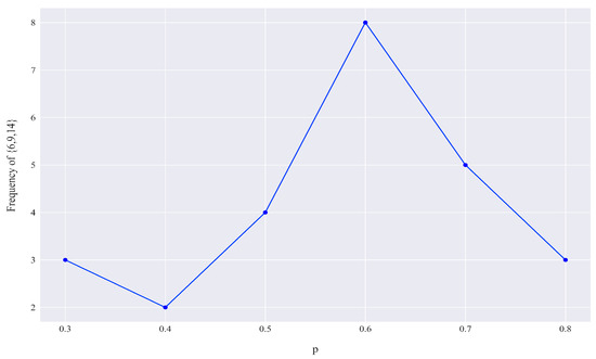
Figure 6. The number of times that {6, 9, 14} are selected under different p.

The experiments show that when the parameter p is chosen around 0.6, i.e., the exploration is located in the middle level, the proposed Geometric Greedy algorithm can achieve the best learning effect. In addition, the algorithm running times are almost the same under different p, which implies that the change of the “geometry factor” does not have a significant impact on the algorithm’s computational efficiency.

4.4. When Resources Are Under-Allocated

The above analysis assumes that disaster emergency materials are abundant, i.e., the emergency resources are sufficient to satisfy the demand at each affected site. However, in the real world, emergency materials are scarce in most cases, especially after a sudden outbreak of natural disasters. A surge in demand puts much stress on the emergency materials warehouses’ inventories.

To simulate the case that resources are under-allocated, We keep the initial inventories in three warehouses invariant and make the demand at each flooding site in each time period rise by 10%, 20%, 30%, 40%, and 50%, respectively, in which cases the disaster emergency materials in the warehouses are not able to satisfy all the demands at each flooding site. The weighted costs (objective values) under increasing demand are illustrated in Figure 7. A marked increase in the objective value can be witnessed as demand inflates. When the demand at each flooding site rises by 50%, the weighted cost doubles more than the cost with no demand inflation. Thus, sufficient emergency materials are critically essential for the reduction in economic losses and the success of emergency operations. Warehouses need to replenish in time to meet the supply demand as much as possible.

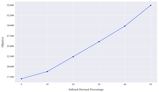
Figure 7. The objective values as demand increases.

5. Conclusions

In this paper, we construct a three-layer emergency logistics network and develop a bi-objective, multi-period stochastic integer programming model for location planning, taking into account the subsequent distribution and allocation of relief supplies under disaster uncertainty. A newly developed Geometric Greedy algorithm is designed to solve this model.

To verify the applicability of our model and algorithms, we use an urban flood disaster in Futian District, Shenzhen, as a case study. Numerical experiments demonstrate that the proposed Geometric Greedy algorithm outperforms the $ϵ$-Greedy and Upper-Confidence-Bound (UCB) algorithms in terms of computational efficiency and convergence stability. Sensitivity analysis on the geometry factor p reveals that the computational efficiency of the Geometric Greedy algorithm remains relatively consistent across different values of p. However, selecting a moderate p can improve the learning outcome by increasing the frequency of identifying the optimal transfer station location plan.

In summary, our research expands the application of reinforcement learning to dynamic disaster response within a three-layer emergency logistics network in uncertain environments. It offers guidelines for emergency authorities regarding the selection of emergency facility locations and the dynamic delivery of emergency materials to multiple disaster sites following the sudden onset of natural disasters.

Appendix A.1. Proof of Theorem 1

Proof. 

We just simply compute the cost function $H(z,t_0,m)$ and want to use $m_{ilj}^k\left(t\right)$ as the minimizing variables.

$$\begin{array}{c}H(z,t_0,m)\hfill \\ =\mathbb{E}\left({\omega }_1\sum _l{f}_l{z}_l+{\omega }_1\sum _{t=t_0}^T\sum _{i,l,k}\xi c_{il}{e}_{il}{m}_{il}^k\left(t\right)\right.\hfill \\ +\left.{\omega }_1\sum _{t=t_0}^T\sum _{l,j,k}\xi c_{lj}{e}_{lj}{m}_{lj}^k\left(t\right)+{\omega }_2\sum _{t=t_0}^T\sum _{j,k}\xi {\beta }_j\left(t\right)S_j^k\left(t\right)\right)\\ =\mathbb{E}\left[{\omega }_1\sum _l{f}_l{z}_l+{\omega }_1\sum _{t=t_0}^T\sum _{i,l,k}\xi c_{il}{e}_{il}{m}_{il}^k\left(t\right)+{\omega }_1\sum _{t=t_0}^T\sum _{l,j,k}\xi c_{lj}{e}_{lj}{m}_{lj}^k\left(t\right)\right.\hfill \\ +\left.{\omega }_2\sum _{t=t_0}^T\sum _{j,k}\xi {\beta }_j\left(t\right)\left(\sum _{s=t_0}^{t-1}{D}_j^k\left(s\right)-\sum _{s=t_0}^{t-1}\sum _l{m}_{ljks}\right)\right]\\ =\mathbb{E}\left({\omega }_1\sum _l{f}_l{z}_l+{\omega }_1\sum _{t=t_0}^T\sum _{i,l,j,k}\xi c_{il}{e}_{il}{m}_{ilj}^k\left(t\right)\right.\hfill \\ \hspace{1em}+\left.{\omega }_1\sum _{t=t_0}^T\sum _{i,l,j,k}\xi c_{lj}{e}_{lj}{m}_{ilj}^k\left(t\right)-\sum _{t=t_0}^T\sum _{i,l,j,k}\sum _{s=t+1}^T{\omega }_2\xi {\beta }_j\left(s\right)m_{ilj}^k\left(s\right)\right)\\ \hspace{1em}+\mathbb{E}\left({\omega }_2\sum _{t=t_0}^T\sum _{j,k}\xi {\beta }_j\left(t\right)\sum _{s=t_0}^{t-1}{D}_j^k\left(s\right)\right)\hfill \\ =\mathbb{E}\left({\omega }_1\sum _l{f}_l{z}_l+\sum _{t=t_0}^T\sum _{i,l,j,k}\xi {\Delta }_{ilj}^k\left(t\right)m_{ilj}^k\left(t\right)\right)\hfill \\ \hspace{1em}+\mathbb{E}\left({\omega }_2\sum _{t=t_0}^T\sum _{j,k}\sum _{s=t_0}^{t-1}\xi {\beta }_j\left(t\right)D_j^k\left(s\right)\right).\hfill \end{array}$$

Since the last term does not involve minimizing variables, $z_l,m_{ilj}^k\left(t\right)$, we shall drop it when considering minimizing H. □

Appendix A.2. Proof of Theorem 2

Proof. 

$$\begin{array}{c}\hspace{1em}\mathbb{P}(D_j^k\left(t\right)>{\lambda }_j^k\left(t\right)+\delta )\hfill \\ =\mathbb{P}[exp\left(t{D}_j^k\left(t\right)\right)>exp\left(t({\lambda }_j^k\left(t\right)+\delta )\right)]\hspace{1em}(t>0)\hfill \\ \le exp[-t({\lambda }_j^k\left(t\right)+\delta )]\mathbb{E}[exp\left(t{D}_j^k\left(t\right)\right)]\hspace{1em}(\mathrm{Chebyshev}’\mathrm{s} \mathrm{Inequality})\hfill \\ =exp[-t({\lambda }_j^k\left(t\right)+\delta )]exp\left[{\lambda }_j^k\left(t\right)({\mathrm{e}}^t-1)\right]\hfill \\ =exp[{\lambda }_j^k\left(t\right){\mathrm{e}}^t-t({\lambda }_j^k\left(t\right)+\delta )-{\lambda }_j^k\left(t\right)]\hfill \end{array}$$

We observe the minimum of ${\lambda }_j^k\left(t\right){\mathrm{e}}^t-t({\lambda }_j^k\left(t\right)+\delta )-{\lambda }_j^k\left(t\right)$ is $\delta -({\lambda }_j^k\left(t\right)+\delta )ln(1+\delta /{\lambda }_j^k\left(t\right))$ and is attained when $t=ln(1+\delta /{\lambda }_j^k\left(t\right))$. Hence, it follows

$$\begin{array}{c}\hspace{1em}\mathbb{P}(D_j^k\left(t\right)>{\lambda }_j^k\left(t\right)+\delta )\hfill \\ \le exp\left[\delta -({\lambda }_j^k\left(t\right)+\delta )ln(1+\delta /{\lambda }_j^k\left(t\right))\right]\hfill \\ \le exp\left[2{(-{\lambda }_j^k\left(t\right)ln(1-\alpha ))}^{1/2}-({\lambda }_j^k\left(t\right)+2{(-{\lambda }_j^k\left(t\right)ln(1-\alpha ))}^{1/2})\right.\\ \hfill ·\left.ln(1+2{(-{\lambda }_j^k\left(t\right)ln(1-\alpha ))}^{1/2})\right]\\ \le exp\left[2{(-ln(1-\alpha ))}^{1/2}-(1+2{(-ln(1-\alpha ))}^{1/2})\right.\hfill \\ \hfill ·\left.ln(1+2{(-ln(1-\alpha ))}^{1/2})\right]\\ \le 1-\alpha .\hfill \end{array}$$

□

References

- Jin, H.; Zhao, Y.; Lu, P.; Zhang, S.; Chen, Y.; Zheng, S.; Zhu, Z. Using Machine Learning to Identify and Optimize Sensitive Parameters in Urban Flood Model Considering Subsurface Characteristics. Int. J. Disaster Risk Sci. 2024, 15, 116–133. [Google Scholar] [CrossRef]
- Seaberg, D.; Devine, L.; Zhuang, J. A review of game theory applications in natural disaster management research. Nat. Hazards 2017, 89, 1461–1483. [Google Scholar] [CrossRef]
- Kalantari, Z.; Ferreira, C.S.S.; Koutsouris, A.J.; Ahlmer, A.K.; Cerdà, A.; Destouni, G. Assessing flood probability for transportation infrastructure based on catchment characteristics, sediment connectivity and remotely sensed soil moisture. Sci. Total Environ. 2019, 661, 393–406. [Google Scholar] [CrossRef]
- Pérez-Rodríguez, N.; Holguín-Veras, J. Inventory-allocation distribution models for postdisaster humanitarian logistics with explicit consideration of deprivation costs. Transp. Sci. 2016, 50, 1261–1285. [Google Scholar] [CrossRef]
- Ministry of Emergence Management of China. National Natural Disasters in the First Three Quarters of 2021. Available online: https://www.mem.gov.cn/xw/yjglbgzdt/202110/t20211010_399762.shtml (accessed on 10 January 2023).
- Zhang, Z.; Liang, J.; Zhou, Y.; Huang, Z.; Jiang, J.; Liu, J.; Yang, L. A multi-strategy-mode waterlogging-prediction framework for urban flood depth. Nat. Hazards Earth Syst. Sci. 2022, 22, 4139–4165. [Google Scholar] [CrossRef]
- Awah, L.; Belle, J.; Nyam, Y.S. A Systematic Analysis of Systems Approach and Flood Risk Management Research: Trends, Gaps, and Opportunities. Int. J. Disaster Risk Sci. 2024, 15, 45–57. [Google Scholar] [CrossRef]
- Xu, H.; Fang, D.; Jin, Y. Emergency logistics theory, model and method: A review and further research directions. In Proceedings of the 2018 3rd International Conference on Communications, Information Management and Network Security (CIMNS 2018), Wuhan, China, 27–28 September 2018; Atlantis Press: Amsterdam, The Netherlands, 2018; pp. 188–192. [Google Scholar]
- Trivedi, A.; Singh, A. Facility location in humanitarian relief: A review. Int. J. Emerg. Manag. 2018, 14, 213–232. [Google Scholar] [CrossRef]
- Yu, D.; Yin, J.; Wilby, R.; Lane, S. Disruption of emergency response to vulnerable populations during floods. Nat. Sustain. 2020, 3, 728–736. [Google Scholar] [CrossRef]
- Tzeng, G.H.; Cheng, H.J.; Huang, T.D. Multi-objective optimal planning for designing relief delivery systems. Transp. Res. Part Logist. Transp. Rev. 2007, 43, 673–686. [Google Scholar] [CrossRef]
- Kleywegt, A.J.; Shapiro, A.; Homem-de Mello, T. The sample average approximation method for stochastic discrete optimization. SIAM J. Optim. 2002, 12, 479–502. [Google Scholar] [CrossRef]
- Gosavi, A. Reinforcement learning: A tutorial survey and recent advances. INFORMS J. Comput. 2009, 21, 178–192. [Google Scholar] [CrossRef]
- Shakya, A.K.; Pillai, G.; Chakrabarty, S. Reinforcement learning algorithms: A brief survey. Expert Syst. Appl. 2023, 231, 120495. [Google Scholar] [CrossRef]
- Zhang, X.; Chen, X.; Ding, Y.; Zhang, Y.; Wang, Z.; Shi, J.; Johansson, N.; Huang, X. Smart real-time evaluation of tunnel fire risk and evacuation safety via computer vision. Saf. Sci. 2024, 177, 106563. [Google Scholar] [CrossRef]
- Chang, M.S.; Tseng, Y.L.; Chen, J.W. A scenario planning approach for the flood emergency logistics preparation problem under uncertainty. Transp. Res. Part E 2007, 43, 737–754. [Google Scholar] [CrossRef]
- Mete, H.O.; Zabinsky, Z.B. Stochastic optimization of medical supply location and distribution in disaster management. Int. J. Prod. Econ. 2010, 126, 76–84. [Google Scholar] [CrossRef]
- Ahmadi, M.; Seifi, A.; Tootooni, B. A humanitarian logistics model for disaster relief operation considering network failure and standard relief time: A case study on San Francisco district. Transp. Res. Part E 2015, 75, 145–163. [Google Scholar] [CrossRef]
- Paul, J.A.; Zhang, M. Supply location and transportation planning for hurricanes: A two-stage stochastic programming framework. Eur. J. Oper. Res. 2019, 274, 108–125. [Google Scholar] [CrossRef]
- Mohammadi, S.; Darestani, S.A.; Vahdani, B.; Alinezhad, A. A robust neutrosophic fuzzy-based approach to integrate reliable facility location and routing decisions for disaster relief under fairness and aftershocks concerns. Comput. Ind. Eng. 2020, 148, 106734. [Google Scholar] [CrossRef]
- Cao, C.J.; Li, C.D.; Yang, Q.; Liu, Y.; Qu, T. A novel multi-objective programming model of relief distribution for sustainable disaster supply chain in large-scale natural disasters. J. Clean. Prod. 2018, 174, 1422–1435. [Google Scholar] [CrossRef]
- Zhan, S.l.; Liu, S.; Ignatius, J.; Chen, D.; Chan, F.T. Disaster relief logistics under demand-supply incongruence environment: A sequential approach. Appl. Math. Model. 2021, 89, 592–609. [Google Scholar] [CrossRef]
- Moreno, A.; Alem, D.; Ferreira, D.; Clark, A. An effective two-stage stochastic multi-trip location-transportation model with social concerns in relief supply chains. Eur. J. Oper. Res. 2018, 269, 1050–1071. [Google Scholar] [CrossRef]
- Holguín-Veras, J.; Pérez, N.; Jaller, M.; Van Wassenhove, L.N.; Aros-Vera, F. On the appropriate objective function for post-disaster humanitarian logistics models. J. Oper. Manag. 2013, 31, 262–280. [Google Scholar] [CrossRef]
- Hu, S.; Han, C.; Dong, Z.S.; Meng, L. A multi-stage stochastic programming model for relief distribution considering the state of road network. Transp. Res. Part B Methodol. 2019, 123, 64–87. [Google Scholar] [CrossRef]
- Kaelbling, L.P.; Littman, M.L.; Moore, A.W. Reinforcement learning: A survey. J. Artif. Intell. Res. 1996, 4, 237–285. [Google Scholar] [CrossRef]
- Su, Z.P.; Jiang, J.G.; Liang, C.Y.; Zhang, G.F. Path selection in disaster response management based on Q-learning. Int. J. Autom. Comput. 2011, 8, 100–106. [Google Scholar] [CrossRef]
- Sarabakha, A.; Kayacan, E. Y6 tricopter autonomous evacuation in an indoor environment using Q-learning algorithm. In Proceedings of the 2016 IEEE 55th Conference on Decision and Control (CDC), Las Vegas, NV, USA, 12–14 December 2016; IEEE: New York, NY, USA, 2016; pp. 5992–5997. [Google Scholar]
- Nadi, A.; Edrisi, A. Adaptive multi-agent relief assessment and emergency response. Int. J. Disaster Risk Reduct. 2017, 24, 12–23. [Google Scholar] [CrossRef]
- Yan, L.; Mahmud, S.; Shen, H.; Foutz, N.Z.; Anton, J. MobiRescue: Reinforcement learning based rescue team dispatching in a flooding disaster. In Proceedings of the 2020 IEEE 40th International Conference on Distributed Computing Systems (ICDCS), Singapore, 29 November–1 December 2020; IEEE: Singapore, 2020; pp. 111–121. [Google Scholar]
- Yu, L.; Zhang, C.; Jiang, J.; Yang, H.; Shang, H. Reinforcement learning approach for resource allocation in humanitarian logistics. Expert Syst. Appl. 2021, 173, 114663. [Google Scholar] [CrossRef]
- Hachiya, D.; Mas, E.; Koshimura, S. A reinforcement learning model of multiple UAVs for transporting emergency relief supplies. Appl. Sci. 2022, 12, 10427. [Google Scholar] [CrossRef]
- Auer, P.; Ortner, R. UCB revisited: Improved regret bounds for the stochastic multi-armed bandit problem. Period. Math. Hung. 2010, 61, 55–65. [Google Scholar] [CrossRef]
- Xinhuanet. 11 People Dead in Shenzhen Floods. Available online: http://en.people.cn/n3/2019/0414/c90000-9566570.html (accessed on 1 December 2021).
- Peixoto, J.P.; Costa, D.; Portugal, P.; Vasques, F. Flood-Resilient Smart Cities: A Data-Driven Risk Assessment Approach Based on Geographical Risks and Emergency Response Infrastructure. Smart Cities 2024, 7, 662–679. [Google Scholar] [CrossRef]
- Sheu, J.B. An emergency logistics distribution approach for quick response to urgent relief demand in disasters. Transp. Res. Part E Logist. Transp. Rev. 2007, 43, 687–709. [Google Scholar] [CrossRef]
- Auer, P.; Cesa-Bianchi, N.; Fischer, P. Finite-time Analysis of the Multiarmed Bandit Problem. Mach. Learn. 2002, 47, 235–256. [Google Scholar] [CrossRef]
Disclaimer/Publisher’s Note: The statements, opinions and data contained in all publications are solely those of the individual author(s) and contributor(s) and not of MDPI and/or the editor(s). MDPI and/or the editor(s) disclaim responsibility for any injury to people or property resulting from any ideas, methods, instructions or products referred to in the content. |
© 2024 by the authors. Licensee MDPI, Basel, Switzerland. This article is an open access article distributed under the terms and conditions of the Creative Commons Attribution (CC BY) license (https://creativecommons.org/licenses/by/4.0/).