Stochastic Complexity of Rayleigh and Rician Data with Normalized Maximum Likelihood

Abstract

The Rician distribution, which arises in radar, communications, and magnetic resonance imaging, is characterized by a noncentrality parameter and a scale parameter. The Rayleigh distribution is a special case of the Rician distribution with a noncentrality parameter of zero. This paper considers generalized hypothesis testing for Rayleigh and Rician distributions using Rissanen’s stochastic complexity, particularly his approximation employing Fisher information matrices. The Rayleigh distribution is a member of the exponential family, so its normalized maximum likelihood density is readily computed, and shown to asymptotically match the Fisher information approximation. Since the Rician distribution is not a member of the exponential family, its normalizing term is difficult to compute directly, so the Fisher information approximation is employed. Because the square root of the determinant of the Fisher information matrix is not integrable, we restrict the integral to a subset of its range, and separately encode the choice of subset.

1. Introduction

In 1978, Schwartz [1] and Rissanen [2] independently addressed the problem of model order estimation. Although they approached the problem from rather different viewpoints—Schwarz from an asymptotic Bayesian viewpoint, Rissanen from a coding-theoretic viewpoint—they landed on similar expressions. Over the next two decades, Rissanen refined his minimum description length principle [3,4,5,6,7], eventually “settling” on stochastic complexity computed with Normalized Maximum Likelihood (NML) codes in 1996 [8]. Technical details concerning NML for continuous probability models are addressed in [9]. Surveys of research in minimum description length and stochastic complexity, as well as the related (and older [10]) concept of minimum message length [11], may be found in [12,13,14,15,16,17,18].

This paper explores generalized hypothesis testing with Rayleigh and Rician models using stochastic complexity. Stochastic complexity offers an approach to hypothesis testing that avoids arbitrary thresholds and having to choose Bayesian prior distributions.

1.1. Normalized Maximum Likelihood

Notation in the style of [19] will be employed throughout, with some simplifications, given that only Rician and Rayleigh distributions are considered. Let $x^n=(x_1,\dots ,x_n)\in {[0,\infty )}^n$ denote a dataset. A particular model class is defined as a set of parameterized densities for $x^n$, denoted $\mathcal{M}=\{f(x^n;\theta ):\theta \in {\mathsf{\Theta }}_{\mathcal{M}}\}$. Let $\widehat{\theta }\left(x^n\right)$ denote the Maximum-Likelihood (ML) estimate of $\theta$, which we assume to be in ${\mathsf{\Theta }}_{\mathcal{M}}$ for all $x^n$.

If the normalizing constant

$$\mathcal{C}\left(\mathcal{M}\right)=\int f({\tilde{x}}^n;\widehat{\theta }({\tilde{x}}^n))d{\tilde{x}}^n$$

(1)

is finite, we can define the NML density for class $\mathcal{M}$ as

$$f_{NML}(x^n;\mathcal{M})={\displaystyle \frac{f(x^n;\widehat{\theta }\left(x^n\right))}{\mathcal{C}\left(\mathcal{M}\right)}}.$$

(2)

Much of this paper will address the challenges of dealing with models for which the integral in (1) is not finite.

The stochastic complexity of the data given a model $\mathcal{M}$ is defined as the negative logarithm of (2):

$$SC\left(\mathcal{M}\right)\stackrel{\mathrm{def}}{=}-ln{f}_{NML}(x^n;\mathcal{M})=-lnf(x^n;\widehat{\theta }\left(x^n\right))+ln\mathcal{C}\left(\mathcal{M}\right).$$

(3)

Here we are using the natural logarithm to express stochastic complexity in “nats”. Dividing the result by $ln\left(2\right)$, or equivalently multiplying by ${log}_e\left(2\right)$, would express the result in “bits”.

Given a competing set of models, one chooses the model that minimizes stochastic complexity. Leaving out the minus sign in (3), one can think about the procedure as maximizing a penalized likelihood, with higher $\mathcal{C}$ penalizing more complex models. This simple description assumes the complexities of the competing models are finite; issues concerning infinite complexities present challenges that will be extensively addressed below.

If (1) is challenging to compute, one may employ the asymptotic approximation (Equation (19) of [8])

$$ln\mathcal{C}\left(\mathcal{M}\right)\approx {\displaystyle \frac{k}{2}}ln{\displaystyle \frac{n}{2\pi }}+ln{\int }_{{\mathsf{\Theta }}_{\mathcal{M}}}\sqrt{\left|I\right(\theta \left)\right|}d\theta ,$$

(4)

where $I\left(\theta \right)$ is the Fisher information matrix for the parameter vector $\theta$ and k is the dimension of ${\mathsf{\Theta }}_{\mathcal{M}}$.

The above exposition assumed the integrals in (1) and (4) are finite; we shall return to this sticky issue—which is the reason we put “settling” in quotes in the first paragraph—in Section 1.3.

1.2. Model Comparison Scenarios

The Rician distribution is parameterized by a noncentrality parameter $a\ge 0$ and a scale parameter ${\sigma }^2>0$; it arises in radar [20,21], communications [22], and magnetic resonance imaging [23,24,25]. The Rayleigh distribution is a special case of the Rician, with $a=0$. In wireless communications, while both distributions can model the effects of numerous scattered paths, the Rician distribution in particular models models data including a strong line-of-sight component.

This paper addresses the question: How can we discriminate between Rayleigh and Rician data using stochastic complexity? Our primary interest is choosing between the Rayleigh and Rician distributions when none of the parameters are assumed known. For instance, in a radar application, the Rician distribution might model the voltage distribution certain kind of target (with a strong specular aspect), and a Rayleigh distribution might model another kind of target (with entirely diffuse aspects) or the absence of a target. If one simply plugged in ML estimates and chose the model with the highest likelihood, the Rician would always be chosen, since it enjoys two degrees of freedom instead of just one. In radar, one generally employs a generalized likelihood ratio test with a threshold chosen to achieve tradeoffs between “probability of detection” and “probability of false alarm”. Stochastic complexity offers an avenue towards choosing between models based on the inherent structure of those models without setting a subjective threshold. One could consider a restricted version of this problem where the ${\sigma }^2$ parameter for both distributions is assumed known, in which case the Rayleigh model has no free parameters and its stochastic complexity is just its negative loglikelihood.

Stochastic complexity may be useful even if the number of parameters is the same for each model. The Poisson and geometric distributions are considered in [26,27], which find that even though they both have a single parameter, for small sample sizes, if we simply choose the model with the largest likelihood, “data generated by the geometric distribution are misclassified as Poisson much more frequently than the other way around.” The Poisson distribution intuitively has more “explanatory” power than the geometric. Using the classic “Bayesian information criterion” penalty of $(k/2)lnn$ (the first term of (4), with $2\pi$ omitted) does not help, since both models have the same number of parameters, whereas the full formula puts both models on an equal footing.

Using stochastic complexity, one could compare a Rayleigh model with unknown ${\sigma }^2$ with a Rician with unknown ${\sigma }^2$ and known a, or known a and unknown ${\sigma }^2$. Or, one could compare two Rician distributions with known ${\sigma }^2$ but different known values of a. These scenarios are less likely in practical applications, but they illustrate the flexibility of the method.

1.3. The Infinity Problem

Unfortunately, for many models of interest—including Rayleigh and Rician models—the integrals in (1) and (4) are not finite when computed over the full parameter space ${\mathsf{\Theta }}_{\mathcal{M}}$ (see Chapter 11 of [14]). The general approach is to artificially restrict the integral to a particular subset. As Wallace and Dowe [28] opine, this “seems arbitrary and distasteful. We are given no general guidance as to how this restriction should be performed and different restrictions give different results.”

In some cases, the limits of the subset may be be taken as hyperparameters, and a second normalization step can be taken over those hyperparameters. If the resulting integral itself is infinite, the process can be repeated with hyper-hyperparameters, and so on. In [29], Rissanen needs to cascade three normalization steps for regression problems in denoising applications. How to conduct such “renormalization” is not always obvious. In Section 4.5 of [27], de Rooij and Grünwald mention that their first attempt at renormalization for Poisson and geometric models resulted in another infinite integral, and that they were unable to conduct a second renormalization. In their study of Gaussian distributions (Section III of ([19]), Hirai and Yamanishi stop after their second normalization; the remaining integral is still infinite over the full range, but they note the resulting stochastic complexity has a weaker dependence over the remaining hyper-hyperparameters than the hyperparameters from the first normalization.

We have been unable to conduct renormalization for Rayleigh and Rician models, so we will employ the strategy of Section V of [8]. We define a set of subsets of ${\mathsf{\Theta }}_{\mathcal{M}}$ whose union covers all of ${\mathsf{\Theta }}_{\mathcal{M}}$ and for which the integral converges for all subsets, compute the integral for the smallest subset containing $\widehat{\theta }\left(x^n\right)$, and add some bits (or nats) to the stochastic complexity to separately encode the choice of subset. This approach is not terrible, but it is unsatisfying, as there is generally no clear “best” way to choose the subsets or how to encode their selection.

2. Rayleigh Data

The probability density of n independent Rayleigh random variables is

$$f(x^n;{\sigma }^2)=\prod _{i=1}^n{\displaystyle \frac{x_i}{{\sigma }^2}}exp\left(-{\displaystyle \frac{x_i^2}{2{\sigma }^2}}\right).$$

(5)

Dropping terms that do not depend on ${\sigma }^2$, the loglikelihood is

$$L\left({\sigma }^2\right)=-nln{\sigma }^2-\sum _{i=1}^n{\displaystyle \frac{x_i^2}{2{\sigma }^2}},$$

(6)

which has the first and second derivatives

$$\begin{array}{cc}\hfill {\displaystyle \frac{dL}{d{\sigma }^2}}\left({\sigma }^2\right)& =-{\displaystyle \frac{n}{{\sigma }^2}}+\sum _{i=1}^n{\displaystyle \frac{x_i^2}{2{\left({\sigma }^2\right)}^2}},\hfill \\ \hfill {\displaystyle \frac{dL}{d{\left({\sigma }^2\right)}^2}}\left({\sigma }^2\right)& ={\displaystyle \frac{n}{{\left({\sigma }^2\right)}^2}}-\sum _{i=1}^n{\displaystyle \frac{x_i^2}{{\left({\sigma }^2\right)}^3}}.\hfill \end{array}$$

(7)

The ML estimate of ${\sigma }^2$ is

$${\widehat{\sigma }}^2\left(x^n\right)={\displaystyle \frac{1}{2n}}\sum _{i=1}^n{x}_i^2.$$

(8)

2.1. Normalized Maximum Likelihood for Rayleigh Data

We follow the approach and notation of Hirai and Yamanishi in their gamma distribution example in Section II.D of [19].

Let $g({\widehat{\sigma }}^2\left(x^n\right);{\sigma }^2)$ denote the density function of the ML estimate for an assumed ${\sigma }^2$; this will allow the normalizing integral (1) to be computed via the ML estimate ${\widehat{\sigma }}^2$ instead of the original n-dimensional data. Since the Rayleigh distribution is a member of the exponential family, we may factor the density of the data as

$$f(x^n;{\sigma }^2)=H(x^n|{\widehat{\sigma }}^2\left(x^n\right))g({\widehat{\sigma }}^2\left(x^n\right);{\sigma }^2),$$

(9)

where

$$H(x^n|{\widehat{\sigma }}^2\left(x^n\right))={\displaystyle \frac{f(x^n;{\sigma }^2)}{g({\widehat{\sigma }}^2\left(x^n\right);{\sigma }^2)}}$$

(10)

is the factor of the data density that is independent of the model parameter ${\sigma }^2$, as explained in Section II.C of [19] (middle of left column).

Multiplying both sides of (8) by $2n$, we see that $2n{\widehat{\sigma }}^2\left(x^n\right)$ is gamma distributed with shape parameter n and scale parameter $2{\sigma }^2$, so

$$g({\widehat{\sigma }}^2\left(x^n\right);{\sigma }^2)={\displaystyle \frac{2n}{{\left(2{\sigma }^2\right)}^n(n-1)!}}{[2n{\widehat{\sigma }}^2\left(x^n\right)]}^{n-1}exp\left(-{\displaystyle \frac{2n{\widehat{\sigma }}^2\left(x^n\right)}{2{\sigma }^2}}\right).$$

(11)

The $2n$ in the numerator of the first factor comes from the mapping of multiplying ${\sigma }^2$ by $2n$. Fix ${\widehat{\sigma }}^2\left(x^n\right)={\widehat{\sigma }}^2$. Then

$$g({\widehat{\sigma }}^2)\stackrel{\mathrm{def}}{=}g({\widehat{\sigma }}^2;{\widehat{\sigma }}^2)={\displaystyle \frac{n^n{e}^{-n}}{{\widehat{\sigma }}^2(n-1)!}}.$$

(12)

Unfortunately, the integral of (12) over its full range is not finite, so following the reasoning of [19], we restrict the integral to run from ${\sigma }_{min}^2>0$ to ${\sigma }_{max}^2<\infty$:

$$\mathcal{C}\left(\mathcal{M}\right)={\int }_{{\sigma }_{min}^2}^{{\sigma }_{max}^2}{\displaystyle \frac{n^n{e}^{-n}}{{\widehat{\sigma }}^2(n-1)!}}d{\widehat{\sigma }}^2={\displaystyle \frac{n^n{e}^{-n}}{(n-1)!}}ln{\displaystyle \frac{{\sigma }_{max}^2}{{\sigma }_{min}^2}}.$$

(13)

Issues related to choosing such limits will appear throughout the rest of the paper; the results are sensitive to such choices.

The natural logarithm of (13) is

$$ln\mathcal{C}\left(\mathcal{M}\right)=nlnn-n-ln(n-1)!+lnln{\displaystyle \frac{{\sigma }_{max}^2}{{\sigma }_{min}^2}}.$$

(14)

Invoking Sterling’s approximation

$$\begin{array}{cc}\hfill ln(n-1)!& \approx (n-1)ln(n-1)-(n-1)+{\displaystyle \frac{1}{2}}ln\left(2\pi [n-1]\right))\hfill \\ \hfill & =nln(n-1)-n+1-{\displaystyle \frac{1}{2}}ln(n-1)+ln2\pi \hfill \end{array}$$

(15)

on (14) yields the approximation

$$ln\mathcal{C}\left(\mathcal{M}\right)\approx nln{\displaystyle \frac{n}{n-1}}-1+{\displaystyle \frac{1}{2}}ln{\displaystyle \frac{n-1}{2\pi }}+lnln{\displaystyle \frac{{\sigma }_{max}^2}{{\sigma }_{min}^2}}.$$

(16)

2.2. Fisher-Based Approximate NML

The Fisher information for the Rayleigh model, $I\left({\sigma }^2\right)$, is

$$I\left({\sigma }^2\right)=-E\left[{\displaystyle \frac{\partial L^2}{\partial {\left({\sigma }^2\right)}^2}}\right]=-{\displaystyle \frac{1}{{\left({\sigma }^2\right)}^2}}+{\displaystyle \frac{E\left[x\right]}{{\left({\sigma }^2\right)}^3}}=-{\displaystyle \frac{1}{{\left({\sigma }^2\right)}^2}}+{\displaystyle \frac{2{\sigma }^2}{{\left({\sigma }^2\right)}^3}}={\displaystyle \frac{1}{{\left({\sigma }^2\right)}^2}}.$$

(17)

The integral of the square root of (17) over the full range of ${\sigma }^2$ is not finite, so as in the previous subsection, we integrate from ${\sigma }_{min}^2$ to ${\sigma }_{max}^2$ to compute the asymptotic approximation

$$ln\mathcal{C}\left(\mathcal{M}\right)\approx {\displaystyle \frac{1}{2}}ln{\displaystyle \frac{n}{2\pi }}+ln{\int }_{{\sigma }_{min}^2}^{{\sigma }_{max}^2}\sqrt{{\displaystyle \frac{1}{{\left({\sigma }^2\right)}^2}}}d{\sigma }^2={\displaystyle \frac{1}{2}}ln{\displaystyle \frac{n}{2\pi }}+lnln{\displaystyle \frac{{\sigma }_{max}^2}{{\sigma }_{min}^2}}.$$

(18)

Note that as $n\to \infty$, the first term in (16) approaches 1, so the first two terms cancel. Approximating $n-1$ as n in the third term of (16) would then yield the same expression as (18).

3. Rician Data

The Rician distribution will be far more challenging to deal with than the Rayleigh distribution. It does not admit a decomposition in terms of a sufficient statistic like in (9), making closed form calculation of the NML density intractable. Additionally, the presence of Bessel functions makes both ML estimation and the computation of Fisher information more difficult.

The probability density of n independent Rician random variables is

$$f(x^n;a,{\sigma }^2)=\prod _{i=1}^n{\displaystyle \frac{x_i}{{\sigma }^2}}exp\left(-{\displaystyle \frac{x_i^2+a^2}{2{\sigma }^2}}\right)I_0\left({\displaystyle \frac{a{x}_i}{{\sigma }^2}}\right).$$

(19)

Dropping terms that do not depend on b or ${\sigma }^2$, the loglikelihood is

$$L(a,{\sigma }^2)=-nln{\sigma }^2-\sum _{i=1}^n{\displaystyle \frac{x_i^2}{2{\sigma }^2}}-n{\displaystyle \frac{a^2}{2{\sigma }^2}}+\sum _{i=1}^{n}ln{I}_0\left({\displaystyle \frac{a{x}_i}{{\sigma }^2}}\right).$$

(20)

The derivatives of (20) with respect to a and ${\sigma }^2$ are

$$\begin{array}{cc}\hfill {\displaystyle \frac{\partial L}{\partial a}}(a,{\sigma }^2)& =-n{\displaystyle \frac{a}{{\sigma }^2}}+\sum _{i=1}^n{\displaystyle \frac{x_i}{{\sigma }^2}}{I}_{1|0}\left({\displaystyle \frac{a{x}_i}{{\sigma }^2}}\right),\hfill \end{array}$$

(21)

$$\begin{array}{cc}\hfill {\displaystyle \frac{\partial L}{\partial {\sigma }^2}}(a,{\sigma }^2)& =-{\displaystyle \frac{n}{{\sigma }^2}}+\sum _{i=1}^n{\displaystyle \frac{x_i^2}{2{\left({\sigma }^2\right)}^2}}+M{\displaystyle \frac{a^2}{2{\left({\sigma }^2\right)}^2}}-\sum _{i=1}^n{\displaystyle \frac{a{x}_i}{{\left({\sigma }^2\right)}^2}}{I}_{1|0}\left({\displaystyle \frac{a{x}_i}{{\sigma }^2}}\right),\hfill \end{array}$$

(22)

where we define modified Bessel function ratios as $I_{u|v}\left(z\right)=I_u\left(z\right)/I_v\left(z\right)$ and we have used the modified Bessel function relations (see, for instance, Equation (1.52) on p. 16 and Equation (1.68) on p. 21 of [30])

$$\begin{array}{ccc}\hfill I_{-n}\left(z\right)& =& I_n\left(\mathrm{f}\mathrm{o}\mathrm{r}\mathrm{i}\mathrm{n}\mathrm{t}\mathrm{e}\mathrm{g}\mathrm{e}\mathrm{r}n\right),\hfill \\ \hfill I_v^{\prime }\left(z\right)& =& {\displaystyle \frac{I_{v-1}\left(z\right)+I_{v+1}\left(z\right)}{2}}.\hfill \end{array}$$

(23)

The entries of the Fisher information matrix

$$I(a,\sigma )=-E\left[\begin{array}{cc}{\displaystyle \frac{{\partial }^{2}L}{\partial a^2}}& {\displaystyle \frac{{\partial }^{2}L}{\partial {\sigma }^2\partial a}}\\ {\displaystyle \frac{{\partial }^{2}L}{\partial {\sigma }^2\partial a}}& {\displaystyle \frac{{\partial }^{2}L}{\partial {\left({\sigma }^2\right)}^2}}\end{array}\right]$$

(24)

are derived in the Appendix A and given by

$$\begin{array}{cc}\hfill -E_r\left[{\displaystyle \frac{{\partial }^{2}L}{\partial {\left({\sigma }^2\right)}^2}}\right]& ={\displaystyle \frac{U(a,{\sigma }^2)}{{\left({\sigma }^2\right)}^3}}-{\displaystyle \frac{a^2}{{\left({\sigma }^2\right)}^2}},\hfill \end{array}$$

(25)

$$\begin{array}{cc}\hfill -E_r\left[{\displaystyle \frac{{\partial }^{2}L}{\partial {\left({\sigma }^2\right)}^2}}\right]& ={\displaystyle \frac{1}{{\left({\sigma }^2\right)}^2}}-{\displaystyle \frac{a^2}{{\left({\sigma }^2\right)}^3}}-{\displaystyle \frac{a^4}{{\left({\sigma }^2\right)}^4}}+{\displaystyle \frac{a^2}{{\left({\sigma }^2\right)}^5}}U(a,{\sigma }^2),\hfill \end{array}$$

(26)

$$\begin{array}{cc}\hfill -E_r\left[{\displaystyle \frac{{\partial }^{2}L}{\partial {\sigma }^2\partial a}}\right]& ={\displaystyle \frac{a}{{\left({\sigma }^2\right)}^2}}+{\displaystyle \frac{a^3}{{\left({\sigma }^2\right)}^3}}-{\displaystyle \frac{a}{{\left({\sigma }^2\right)}^4}}U(a,{\sigma }^2),\hfill \end{array}$$

(27)

where

$$\begin{array}{c}\hfill U(a,{\sigma }^2)={\int }_0^{\infty }{x}^{3}exp\left(-{\displaystyle \frac{x^2+a^2}{2{\sigma }^2}}\right){\displaystyle \frac{I_1^2(ax/{\sigma }^2)}{I_0(ax/{\sigma }^2)}}dx.\end{array}$$

(28)

We are unaware of a closed-form expression for (28) and were unable to find any elegant and accurate approximations. The numeric results in this paper use the integral function of Octave version 10.3 with its default settings.

For $a=0$, (25) simplifies to the Fisher information for the Rayleigh case given in (17), and (27) is zero.

Section 3.1 considers scenarios where a is unknown but ${\sigma }^2$ is known. Section 3.2 considers scenarios where ${\sigma }^2$ is unknown but a is known. These two scenarios are less likely encountered in practical applications, but they help build understanding towards scenarios where both a and ${\sigma }^2$ are unknown, which is considered in Section 3.3 and the main focus on this paper. Monte Carlo simulations related to this scenario are presented in Section 4.

3.1. Unknown a, Known ${\sigma }^2$

We first consider the case where ${\sigma }^2$ is assumed known. Setting (21) equal to zero yields the necessary condition for a maximizer; $\widehat{a}\left(x^n\right)$ is the a that satisfies

$$a={\displaystyle \frac{1}{n}}\sum _{i=1}^n{x}_i{I}_{1|0}\left({\displaystyle \frac{a{x}_i}{{\sigma }^2}}\right).$$

(29)

The fixed-point iteration

$$a_{new}={\displaystyle \frac{1}{n}}\sum _{i=1}^n{x}_i{I}_{1|0}\left({\displaystyle \frac{a_{old}{x}_i}{{\sigma }^2}}\right)$$

(30)

converges to the maximizing a.

The Rician distribution is not a member of the exponential family and does not allow a sufficient statistic, so we cannot employ the method demonstrated in Section 1.1. Hence, we immediately turn to Rissanen’s asymptotic approximation. The square root of the Fisher information $I\left(a\right)$, the upper left element of (24), is not integrable over its full range; it admits a lower limit on a of 0, but not an upper limit of ∞. One can restrict the upper limit to a choice of $a_{max}$ and add another term to the complexity associated with encoding $a_{max}$.

Figure 1 plots $\sqrt{I\left(a\right)}$ as a function of a for four different values of ${\sigma }^2$. The integral of $\sqrt{I\left(a\right)}$ from 0 to $a_{max}$, plotted as a function of $a_{max}$, is shown in Figure 2a; its natural logarithm, corresponding to the integral term in the stochastic complexity expression, is shown in Figure 2b.

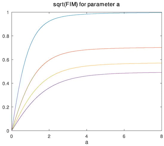
Figure 1. Plot of $\sqrt{I\left(a\right)}$ vs. a assuming ${\sigma }^2$ is known. Different lines, from top to bottom, correspond to ${\sigma }^2=1$, 2, 3, and 4.

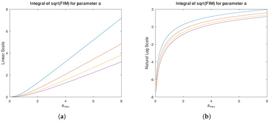
Figure 2. (a) Plot of integral of $\sqrt{I\left(a\right)}$ from 0 to $a_{max}$ vs. $a_{max}$ assuming ${\sigma }^2$ is known. Lines, from top to bottom, correspond to ${\sigma }^2=1,2,3,$ and 4. (b) Natural logarithm of the same integral.

3.2. Unknown ${\sigma }^2$, Known a

We next consider the case where a is assumed known. Although this case is likely not as common in practical applications, we consider it for completeness and as a stepping stone to consider the full case where both a and ${\sigma }^2$ are known.

Setting (22) equal to zero gives the necessary conditions for a maximizer; ${\widehat{\sigma }}^2$ is the ${\sigma }^2$ that satisfies

$${\sigma }^2={\displaystyle \frac{1}{2n}}\sum _{i=1}^n{x}_i^2+{\displaystyle \frac{a^2}{2}}-{\displaystyle \frac{a}{n}}\sum _{i=1}^n{x}_i{I}_{1|0}\left({\displaystyle \frac{a{x}_i}{{\sigma }^2}}\right).$$

(31)

The square root of the Fisher information $I\left({\sigma }^2\right)$, the lower right element of (24), is not integrable over its full range, and it manifests a singularity at ${\sigma }^2=0$. Like in the Rayleigh case, we can limit the integral to a range $[{\sigma }_{min}^2,{\sigma }_{max}^2]$ and add another term to the complexity associated with encoding ${\sigma }_{min}^2$ and ${\sigma }_{max}^2$.

Figure 3 plots $\sqrt{I\left({\sigma }^2\right)}$ as a function of ${\sigma }^2$ for four different values of a. The horizontal axis of Figure 3a runs from 1 to 5; the horizontal axis of Figure 3b runs from 0.1 to 1 to better show detail, in particular the crossing of the $a=0.6$ and $a=0.3$ lines. Exploring this further, Figure 4 plots $\sqrt{I\left({\sigma }^2\right)}$ as a function of a for three different values of ${\sigma }^2$. Notice these functions are not monotonic; they are all largest at $a=0$ and each has minimum. This suggests that for any particular true ${\sigma }^2$, there is an associated a that would give the yield the worst Cramér-Rao lower bound, and $a=0$ would yield the best.

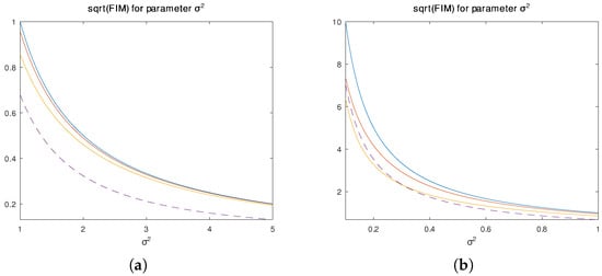
Figure 3. Plots of $\sqrt{I\left({\sigma }^2\right)}$ vs. ${\sigma }^2$ assuming a is known. Solid lines, from top to bottom, correspond to $a=0,0.3$, and $0.6$. The dashed line corresponds to $a=3$. (a) ${\sigma }^2$ ranges from 1 to 5. (b) ${\sigma }^2$ ranges from 0 to 1.

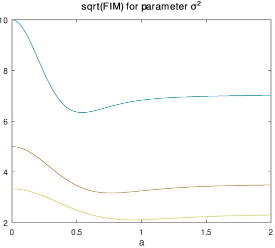
Figure 4. Plot of $\sqrt{I\left({\sigma }^2\right)}$ vs. a assuming a is known. Different lines, from top to bottom, correspond to ${\sigma }^2=0.1$, 0.2, and 0.3.

3.3. Unknown a and Unknown ${\sigma }^2$

If we must co-estimate a and ${\sigma }^2$, we can fold (29) into (31), yielding the simplified condition

$${\sigma }^2={\displaystyle \frac{1}{2n}}\sum _{i=1}^n{x}_i^2-{\displaystyle \frac{a^2}{2}}.$$

(32)

We in turn substitute (32) into (29), which gives the single necessary condition for a

$$a={\displaystyle \frac{1}{n}}\sum _{i=1}^n{x}_i{I}_{1|0}\left[{\displaystyle \frac{a{x}_i}{\frac{1}{2n}{\sum }_{i=1}^n{x}_i^2-\frac{a^2}{2}}}\right].$$

(33)

The ML estimate $\widehat{a}$ can be found with a simple fixed-point iteration

$$a_{new}={\displaystyle \frac{1}{n}}\sum _{i=1}^n{x}_i{I}_{1|0}\left({\displaystyle \frac{a_{old}{x}_i}{\frac{1}{2n}{\sum }_{i=1}^n{x}_i^2-\frac{a_{old}^2}{2}}}\right).$$

(34)

Once the ML estimate for a is found, the ML estimate for ${\sigma }^2$ can be computed according to

$${\widehat{\sigma }}^2={\displaystyle \frac{1}{2n}}\sum _{i=1}^n{x}_i^2-{\displaystyle \frac{{\widehat{a}}^2}{2}}.$$

(35)

Figure 5a plots the double integral

$${\int }_0^{a_{max}}{\int }_{{\sigma }_{min}^2}^{{\sigma }_{max}^2}detI(a,{\sigma }^2)d{\sigma }^{2}da$$

(36)

as a function of $a_{max}$. We choose ${\sigma }_{max}^2=c>1$ and ${\sigma }_{min}^2=1/c$, and plot several lines for different choices of c. This restriction to the range $[1/c,c]$ is inspired by Rissanen’s approach to exponential densities in Section V of [8]. The natural logarithm of Figure 5a, which corresponds to the integral term in the stochastic complexity expression, is shown in Figure 5b.

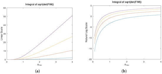
Figure 5. (a) Plot of integral of $\sqrt{detI(a,{\sigma }^2)}$ from 0 to $a_{max}$ (over a) and from $1/c$ to c (over ${\sigma }^2$) vs. $a_{max}$. Lines, from bottom to top, correspond to $c=2$, 4, 6, and 8. (b) Natural logarithm of the same integral.

4. Example

Figure 6 illustrates the probability of correctly detecting a Rician model using stochatic complexity, as a function of a (from 0.05 to 2.5 with a spacing of 0.05), with ${\sigma }^2=2$, estimated using 200,000 Monte Carlo runs per point. This experiment characterizes how the difficulty of distinguishing between Rician and Rayleigh distributions decreases with increasing noncentrality parameter a of the Rician distribution. The solid line corresponds to $n=30$; the dotted line corresponds to $n=100$. If only the loglikelihoods are compared, the Rician model is always chosen since it has an additional degree of freedom.

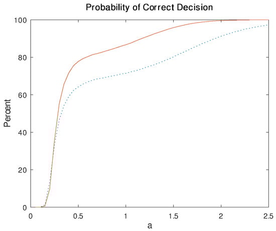
Figure 6. Estimated probability (using 200,000 Monte Carlo runs) of correctly choosing the Rician model using stochastic complexity as a function of the true parameter a for ${\sigma }^2=2$. The lines correspond to $n=30$ (dotted) and $n=100$ (solid).

For the Rayleigh model, we follow Rissanen’s choice for the exponential models in Section V of [8] and restrict the integral over the square root of the Fisher information to the range $[2^{-b_0},2^{b_0}]$, where $b_0$ is the smallest positive integer such that the ML estimate ${\widehat{\sigma }}_0^2\left(x^n\right)\in [2^{-b_0},2^{b_0}]$. (We add a subscript in this section to avoid confusion with the estimate for the Rician case). The natural log of the integral is then

$$ln{\int }_{2^{-b_0}}^{2_0^b}{\displaystyle \frac{1}{{\sigma }^2}}d\theta =lnln{\displaystyle \frac{2_0^b}{2^{-b_0}}}=lnln{2}^{2b_0}=ln(2b_{0}ln2)=ln\left(2b_0\right)+lnln2.$$

(37)

Further following Rissanen [8], we encode $b_0$ with ${log}^{★}\left(b_0\right)+c$ bits, where ${log}^{*}$ is the iterative algorithm computed using base 2, $c\approx 2.87$, and we multiply by $ln2$ to convert to nats.

The stochastic complexity expression for the Rayleigh model is then

$$SC\left(M_{Rayleigh}\right)=-L\left({\widehat{\sigma }}_0^2\right)+{\displaystyle \frac{k}{2}}ln{\displaystyle \frac{n}{2\pi }}+ln\left(2b_0\right)+lnln2+[{log}^{★}\left(b_0\right)+c]ln2.$$

(38)

For the Rician model, we follow the same choice as in the Rayleigh case, restricting the integral over ${\sigma }^2$ to the range $[2^{-b_1},2^{b_1}]$, where $b_1$ is the smallest positive integer such that the ML estimate ${\widehat{\sigma }}_1^2\left(x^n\right)\in [2^{-b_1},2^{b_1}]$ (now using a 1 subscript instead of 0 to avoid confusion with the Rayleigh case). We follow a similar pattern and restrict the integral over a to the range $[0,2^s]$, where s is the smallest positive integer such that the ML estimate $\widehat{a}\left(x^n\right)\in [0,2^s]$. We separately encode $b_1$ and s using the $lo{g}^{★}$ approach we used in the Rayleigh case. We emphasize that different choices of subsets to force integrals to be finite, and the different methods of encoding the chosen subset, will yield different procedures, and there is at present little guidance on how to make such choices. This is addressed further in Section 5.

The stochastic complexity expression for the Rician model is then

$$\begin{array}{cc}\hfill SC\left(M_{Rician}\right)=& -L(\widehat{a},{\widehat{\sigma }}_1^2)+{\displaystyle \frac{k}{2}}ln{\displaystyle \frac{n}{2\pi }}+ln{\int }_0^{2^s}{\int }_{2^{-b_1}}^{2^{b_1}}detI(a,{\sigma }^2)d{\sigma }^{2}da\hfill \\ \hfill & +[{log}^{★}\left(b_1\right)+c]ln2+[{log}^{★}\left(s\right)+c]ln2.\hfill \end{array}$$

(39)

To save computation, we precomputed the log integral term in (39) for $s=1,\dots ,3$ and $b_1=1,\dots ,3$, as shown in Table 1.

Table 1. Precomputed log integral term in (39).

	${\mathit{b}}_1=1$	${\mathit{b}}_1=2$	${\mathit{b}}_1=3$
$s=1$	−0.8218	1.1247	2.8939
$s=2$	0.7067	2.3601	3.9341
$s=3$	1.7426	3.2889	4.7841

5. Conclusions

This paper developed expressions for the NML-based stochastic complexity of Rayleigh models with unknown scale parameter and three cases of Rician models: (1) the noncentrality parameter is unknown, but the scale parameter is assumed to be known; (2) the scale parameter is unknown, but the noncentrality parameter is assumed to be known; and (3) both the noncentrality and scale parameters are unknown. The resulting integrals of the square root of the determinant of the Fisher information matrix diverge when taken over their full range. To address this, we limited the range of the integrals, and separately encoded the choice of range. For the third case, we formulated an encoding scheme inspired by Rissanen [8] and used a Monte Carlo analysis to illustrate how the difficulty of correctly choosing a Rician model changes with the noncentrality parameter of that model.

The primary hope of this paper is to spur further research into stochastic complexity in cases where normalizing integrals are infinite when computed over their full range, particularly for distributions other than the Gaussian. To our knowledge, the only published details of “renormalized maximum likelihood” ([19,29,31]) have involved Gaussian distributions (de Rooij and Grünwald [27] only mention their attempts regarding geometric and Poisson distributions in passing). Perhaps an interested reader can uncover a renormalization scheme for the Rician distribution that we were unable to formulate.

Along with finding renormalization schemes, another line of research would be to find less arbitrary ways of choosing the sets of subsets of the parameter space (along the lines of Section V of [8]) that allow the normalizing integrals to be finite (along with appropriate encoding of the selected subset).

It is remarkable that almost two decades after Rissanen introduced his asymptotic formula for stochastic complexity based on the Fisher information matrix, there is as of yet no general satisfying solution to the “infinity problem”.

The minimum description length principle, in its many forms, selects models, but does not provide any alternative to choosing parameters for those models beyond the classical ML estimate. An alternative philosophy, Minimum Message Length (MML) [10], simultaneously chooses models along with their estimated parameters, and the MML parameter estimates differ from ML estimates. To our knowledge, MML has not been applied to Rayleigh or Rician models. MML requires choosing Bayesian priors; our focus on stochastic complexity has been motivated by a desire to avoid selecting prior distributions.

A natural direction for future work would be to apply these techniques to real data. In [32,33,34], a zero-mean complex “conditionally Gaussian” model, which is functionally equivalent to a Rayleigh model, is employed in building automatic target recognition libraries for synthetic aperture radar data. A similar approach is taken to high-resolution range profile data in [35]. This model is most appropriate for diffuse targets. To incorporate specular reflections, Ref. [36] extended the approach to a Rician model; the authors wrote: “…the performance under the Rician model suffers with smaller training sets. Due to the smaller number of distribution parameters, the conditionally Gaussian approach is able to yield a better performance for any fixed complexity.” A model order estimation technique such as stochastic complexity may help alleviate such issues with overfitting, allowing the library creation process to only choose a Rician model when warranted.

There are many other examples of hierarchies of probability densities, where one density is a special case of the other, in which stochastic complexity could be used to determine if the more complicated density is truly warranted. For instance, the one-parameter exponential distribution is a special case of the two-parameter Weibull distribution, and three-parameter [37,38,39] and four-paremeter [40] generalizations of the Weibull distribution have been proposed. The exponential distribution is also a special case of the two-parameter gamma distribution, which has a three-parameter generalization [41]. Besides exploring hierarchies of models with differing numbers of parameters, stochastic complexity could be used to compare the two-parameter Weibull with the two-parameter gamma; even though they have the same number of parameters, one may have greater explanatory power and be unfairly favored in naive likelihood comparisons.

References

- Schwarz, G. Estimating the Dimension of a Model. Ann. Stat. 1978, 6, 461–464. [Google Scholar] [CrossRef]
- Rissanen, J. Modeling by Shortest Data Description. Automatica 1978, 14, 465–471. [Google Scholar] [CrossRef]
- Rissanen, J. A Universal Prior for Integers and Estimation by Minimum Description Length. Ann. Stat. 1983, 11, 416–431. [Google Scholar] [CrossRef]
- Rissanen, J. Universal Coding, Information, Prediction, and Estimation. IEEE Trans. Inf. Theory 1984, 30, 629–636. [Google Scholar] [CrossRef]
- Rissanen, J. Stochastic Complexity and Modeling. Ann. Stat. 1986, 14, 1080–1100. [Google Scholar] [CrossRef]
- Rissanen, J. Stochastic Complexity. J. R. Stat. Soc. B 1987, 49, 223–239. [Google Scholar] [CrossRef]
- Rissanen, J. Stochastic Complexity in Statistical Inquiry; World Scientific Publishing Co.: New York, NY, USA, 1989. [Google Scholar]
- Rissanen, J. Fisher Information and Stochastic Complexity. IEEE Trans. Inf. Theory 1996, 42, 40–47. [Google Scholar] [CrossRef]
- Suzuki, A.; Yamanishi, K. Foundation of Calculating Normalized Maximum Likelihood for Continuous Probability Models. arXiv 2014, arXiv:2409.08387. [Google Scholar]
- Wallace, C.; Boulton, D. An Information Measure for Classification. Comput. J. 1968, 11, 195–209. [Google Scholar] [CrossRef]
- Wallace, C. Statistical and Inductive Inference by Minimum Message Length; Springer: Berlin/Heidelberg, Germany, 2005. [Google Scholar]
- Grünwald, P. Model Selection Based on Minimum Description Length. J. Math. Psychol. 2000, 44, 133–152. [Google Scholar] [CrossRef] [PubMed]
- Grünwald, P.; Roos, T. Minimum Description Length Revisited. Int. J. Math. Ind. 2020, 11, 1930001. [Google Scholar] [CrossRef]
- Grünwald, P. The Minimum Description Length Principle; MIT Press: Cambridge, MA, USA, 2007. [Google Scholar]
- Rissanen, J. Information and Complexity in Statistical Modeling; Springer: Berlin/Heidelberg, Germany, 2007. [Google Scholar]
- Rissanen, J. Optimal Estimation of Parameters; Cambridge University Press: Cambridge, UK, 2012. [Google Scholar]
- Myung, J.; Navarro, D.; Pitt, M. Model Selection by Normalized Maximum Likelihood. J. Math. Psychol. 2006, 50, 167–179. [Google Scholar] [CrossRef]
- Lanterman, A. Schwarz, Wallace, and Rissanen: Intertwining Themes in Theories of Model Order Estimation. Int. Stat. Rev. 2001, 69, 185–212. [Google Scholar] [CrossRef]
- Hirai, S.; Yamanishi, K. Computation of Normalized Maximum Likelihood Codes for Gaussian Mixture Models with Its Applications to Clustering. IEEE Trans. Inf. Theory 2013, 59, 7718–7727. [Google Scholar] [CrossRef]
- Fried, D. Statistics of the laser radar cross section of a randomly rough target. J. Opt. Soc. Am. 1976, 66, 1150–1160. [Google Scholar] [CrossRef]
- Song, X.; Blair, W.; Willett, P.; Zhou, S. Dominant-plus-Rayleigh Models for RCS: Swerling III/IV versus Rician. IEEE Trans. Aerosp. Electron. Syst. 2013, 49, 2058–2064. [Google Scholar] [CrossRef]
- Wang, L.C.; Liu, W.C.; Cheng, Y.H. Statistical Analysis of a Mobile-to-Mobile Rician Fading Channel Model. IEEE Trans. Veh. Technol. 2009, 58, 32–38. [Google Scholar] [CrossRef]
- Gudbjartsson, H.; Patz, S. The Rician Distribution of Noisy MRI Data. Magn. Reson. Med. 1995, 34, 910–914. [Google Scholar] [CrossRef] [PubMed]
- Sjibers, J.; den Dekker, A.; Scheunders, P.; Dyck, D.V. Maximum-Likelihood Estimation of Rician Distribution Parameters. IEEE Trans. Med. Imaging 1998, 17, 357–361. [Google Scholar] [CrossRef]
- Sjibers, J.; den Dekker, A.; Raman, E.; Dyck, D.V. Parameter Estimation from Magnitude MR Images. Int. J. Imaging Syst. Technol. 1999, 10, 109–114. [Google Scholar] [CrossRef]
- Lanterman, A. Hypothesis Testing for Poisson versus Geometric Distributions using Stochastic Complexity. In Advances in Minimum Description Length: Theory and Applications; Grunwald, P., Myung, I., Pitt, M., Eds.; MIT Press: Cambridge, MA, USA, 2005; Chapter 4; pp. 99–123. [Google Scholar]
- de Rooij, S.; Grünwald, P. An empirical study of minimum description length model selection with infinite parametric complexity. J. Math. Psychol. 2006, 50, 180–192. [Google Scholar] [CrossRef]
- Wallace, C.; Dowe, D. Refinements of MDL and MML Coding. Comput. J. 1999, 42, 330–337. [Google Scholar] [CrossRef]
- Rissanen, J. MDL Denoising. IEEE Trans. Inf. Theory 2000, 7, 2537–2543. [Google Scholar] [CrossRef]
- Tranter, C.J. Bessel Functions with Some Physical Applications; The English University Press Ltd.: London, UK, 1968. [Google Scholar]
- Maanan, S.; Dumitrescu, B.; Girucăneanu, C. Renormalized Maximum Likelihood for Multivariate Autoregressive Models. In Proceedings of the 24th European Signal Processing Conference (EUSIPCO), Budapest, Hungary, 28 August–2 September 2016; pp. 150–154. [Google Scholar]
- O’Sullivan, J.; DeVore, M.; Kedia, V.; Miller, M. Automatic Target Recognition Performance for SAR Imagery Using a Conditionally Gaussian Model. IEEE Trans. Aerosp. Electron. Syst. 2001, 37, 91–108. [Google Scholar] [CrossRef]
- Devore, M.; O’Sullivan, J. Performance Complexity Study of Several Approaches to Automatic Target Recognition from SAR Images. IEEE Trans. Aerosp. Electron. Syst. 2002, 38, 632–648. [Google Scholar]
- Devore, M.; O’Sullivan, J. Quantitative Statistical Assessment of Conditional Models for Synthetic Aperture Radar. IEEE Trans. Image Process. 2004, 13, 113–125. [Google Scholar] [CrossRef] [PubMed]
- Jacobs, S.; O’Sullivan, J. Automatic Target Recognition Using Sequences of High Resolution Radar Range-Profiles. IEEE Trans. Aerosp. Electron. Syst. 2000, 36, 364–382. [Google Scholar] [CrossRef]
- DeVore, M.; Lanterman, A.; O’Sullivan, J. ATR Performance of a Rician Model for SAR Images. In Proceedings of the Automatic Target Recognition X, Orlando, FL, USA, 26–28 April 2000; Volume SPIE Proc. 4050; Sadjadi, F., Ed.; SPIE: Bellingham, WA, USA, 2000. [Google Scholar]
- Mudhokar, G.; Srivastava, D. The Exponentiated Weibull Family for Analyzing Bathtub Failure-Rate Data. IEEE Trans. Reliab. 1993, 42, 299–302. [Google Scholar] [CrossRef]
- Mudhokar, G.; Srivastava, D.; Freimer, M. The Exponentiated Weibull Family: A Reanalysis of the Bus-Motor-Failure Data. Technometrics 1995, 37, 436–445. [Google Scholar] [CrossRef]
- Mudhokar, G.; Srivastava, D.; Kollia, G. A Generalization of the Weibull Distribution with Application to the Analysis of Survival Data. J. Am. Stat. Assoc. 1996, 91, 1575–1583. [Google Scholar] [CrossRef]
- Cordeiro, G.; Biazatti, E.; de Santana, L. A New Extended Weibull Distribution with Application to Influenza and Hepatitis Data. Stats 2023, 6, 657–673. [Google Scholar] [CrossRef]
- Stacy, E. A Generalization of the Gamma Distribution. Ann. Math. Stat. 1962, 33, 1187–1192. [Google Scholar] [CrossRef]
- Heatley, A.H. Some Integrals, Differential Equations, and Series Related to the Modified Bessel Function of the First Kind; University of Toronto Press: Toronto, ON, Canada, 1939. [Google Scholar]
- Idier, J.; Collewet, G. Properties of Fisher Information for Rician Distributions and Consequences in MRI; Research Report hal-01072813v1; HAL: Lyon, France, 2014. [Google Scholar]
Disclaimer/Publisher’s Note: The statements, opinions and data contained in all publications are solely those of the individual author(s) and contributor(s) and not of MDPI and/or the editor(s). MDPI and/or the editor(s) disclaim responsibility for any injury to people or property resulting from any ideas, methods, instructions or products referred to in the content. |
© 2025 by the author. Licensee MDPI, Basel, Switzerland. This article is an open access article distributed under the terms and conditions of the Creative Commons Attribution (CC BY) license.