Estimating the Ratio of Means in a Zero-Inflated Poisson Mixture Model

Abstract

The problem of estimating the ratio of the means of a two-component Poisson mixture model is considered, when each component is subject to zero-inflation, i.e., excess zero counts. The resulting zero-inflated Poisson mixture (ZIPM) model can be viewed as a three-component Poisson mixture model with one degenerate component. The EM algorithm is applied to obtain frequentist estimators and their standard errors, the latter determined via an explicit expression for the observed information matrix. As an intermediate step, we derive an explicit expression for standard errors in the two-component Poisson mixture model (without zero-inflation), a new result. The ZIPM model is applied to simulated data and real ecological count data of frigatebirds on the Coral Sea Islands off the coast of Northeast Australia.

1. Introduction

Baker and Holdsworth (2013) [1] present data relevant to the determination of the relative abundances of two subspecies of frigatebirds (FB), least (LFB) and greater (GFB), in the Coral Sea Islands off the coast of Northeast Australia. The available data is indirect, consisting only of counts of nests in several standardized sites over several time points, rather than direct observations of individuals. Furthermore, the nests of LFB and GFB usually are indistinguishable, (possibly) differing only in their relative numbers per site. Thus, to infer the type of nest one may use techniques from model-based clustering, such as a finite mixture model [2]. In the presence of count data (such as ours), a finite mixture of Poisson distributions is a common choice [3,4]. Previous authors have studied identifiability and estimation of this and related models (e.g., [2]). Given inferred nest type, ecologists may be interested in estimating other qualities of the ecosystem: If the expected numbers of nests per site for LFB and GFB are denoted by $\mu$ and $\nu$ respectively, in this paper we study estimation of their ratio, $\theta \equiv \mu /\nu$, where $0<\theta <\infty$.

Several complications arise. Because no further constraint can be imposed on $\theta$ a priori, the problem is unidentifiable as stated, i.e., $(\mu ,\nu )$ is indistinguishable from $(\nu ,\mu )$. However, LFB are less prevalent than GFB (based on available labeled data, see [1]), which will render the model identifiable; see the second paragraph below. Furthermore, it is typical of such field studies that zero counts are recorded for reasons other than true absence, such as short study periods, secretive or small species, or other uncontrollable factors. In such cases, it is necessary to model the excessive zero-counts directly to not contaminate other inferences [5]. As is commonly done, we shall adopt the zero-inflated Poisson (ZIP) distribution to represent this feature [6,7,8].

We now state a probability model based on a finite mixture model of zero-inflated Poisson distributions to represent the aforementioned scenario: Let $Y_j$ indicate whether LFB ($Y_j=1$) or GFB ($Y_j=0$) are observed in time point j. Let $M_{ij}$ be the actual number of FB nests at site i in time point j (which may not be directly observed due to zero-inflation). Let $Z_{ij}$ indicate whether nest counts are directly observed ($Z_{ij}=1$) or subject to zero-inflation and hence lost ($Z_{ij}=0$). Finally, let $N_{ij}$ denote the number of FB nests observed at site i at time point j. Let $\mathcal{I}\equiv \{1,\dots ,I\}$ and $\mathcal{J}\equiv \{1,\dots ,J\}$ be the corresponding index sets, and set $\mathcal{K}=\mathcal{I}\times \mathcal{J}$, $K=\left|\mathcal{K}\right|=IJ$. For $(i,j)\in \mathcal{K}$, consider random variables (rvs),

$$\hspace{1em}\hspace{1em}\hspace{1em}{Y}_j\sim \mathrm{Bernoulli}\left(\pi \right),$$

(1)

$$\hspace{1em}\hspace{1em}\hspace{1em}\hspace{1em}\hspace{1em}\hspace{1em}\hspace{1em}\hspace{1em}\hspace{1em}{M}_{ij}|Y_j\sim \mathrm{Poisson}\left\{t_i[(1-0^{Y_j})\mu +0^{Y_j}\nu ]\right\},$$

(2)

$$\hspace{1em}\hspace{1em}\hspace{1em}{Z}_{ij}\sim \mathrm{Bernoulli}\left(ϵ\right),$$

(3)

$$\hspace{1em}{N}_{ij}=Z_{ij}{M}_{ij};$$

(4)

where $0^0=1$, $\left\{Y_j\right\}$ and $\left\{Z_{ij}\right\}$ are mutually independent, and $\left\{M_{ij}\right\}$ and $\left\{Z_{ij}\right\}$ are conditionally mutually independent given $\left\{Y_j\right\}$. Thus $M_{ij}$ is a π- mixture of $\mathrm{Poisson}\left(t_i\mu \right)$ and $\mathrm{Poisson}\left(t_i\nu \right)$ rvs, where each $t_i>0$ is known, potentially reflecting a feature of each site common to all time points, and $\mu ,\nu \in (0,\infty )$ are unknown. Further, $N_{ij}$ is a zero-inflated Poisson mixture (ZIPM) rv with zero-inflation parameter $1-ϵ\in (0,1)$ (One may ask if a conditional ZIPM model is equivalent to the well-studied Zero-Truncated Poisson model. We demonstrate that this is not the case in Appendix A).

The main objective of this paper is the problem of estimating the ratio $\theta \equiv \mu /\nu$ based solely on the observed data $\left\{N_{ij}\right\}$, with $\left\{Y_j\right\}$, $\left\{M_{ij}\right\}$, and $\left\{Z_{ij}\right\}$ unobserved. As noted above, for identifiability of $(\mu ,\nu )$, and therefore of $\theta =\mu /\nu$, a restriction must be imposed: we assume that $0<\pi \le 1/2$, corresponding to the knowledge that LFB occurs no more frequently than GFB. We propose frequentist estimation of $\theta$ via the EM algorithm and approximate standard errors via explicit calculation of the observed information matrix (A Bayesian analysis of this same problem can be found in a preprint version of this paper: M. D. Perlman (2022). Estimating the ratio of means in a zero-inflated Poisson mixture model. arXiv:math 2203.13994).

The rest of this paper is organized as follows: In Section 2, we briefly provide notation. In Section 3, we present a preliminary problem of estimating $\theta$ in a standard, two-component Poisson mixture model (i.e., $\left\{Y_j\right\}$ are unobserved and $\left\{M_{ij}\right\}$ are observed, without zero-inflation) to serve as a guidepost for the main problem. Therein, we estimate $\theta$ in a frequentist context via EM and approximate standard errors via explicit calculation of the observed information matrix, which to our knowledge is a new result (Approximate methods are usually used, such as the SEM algorithm [9] or the bootstrap [4]). In Section 4 we address the main problem of estimating the ratio of Poisson means in a zero-inflated Poisson mixture (ZIPM) model, as described in the previous paragraph. In Section 5 the ZIPM model is applied both to simulated data and real data on frigatebirds in the Coral Sea Islands. The results of this study are summarized in Section 6.

2. Notation

Column vectors and arrays denoted by Roman letters appear in bold type, their components in plain type; caps denote rvs:

$$\begin{array}{cc}\hfill \mathbf{t}& \equiv {(t_1,\dots ,t_I)}^{\prime }\in {\mathbb{R}}^I,\hfill \\ \hfill \mathbf{y}& \equiv {(y_1,\dots ,y_J)}^{\prime }\in {\{0,1\}}^J,\hfill & \hfill \mathbf{Y}& \equiv {(Y_1,\dots ,Y_J)}^{\prime }\in {\{0,1\}}^J,\hfill \\ \hfill \mathbf{z}& \equiv \left(z_{ij}\right)\in {\{0,1\}}^{\mathcal{K}},\hfill & \hfill \mathbf{Z}& \equiv \left(Z_{ij}\right)\in {\{0,1\}}^{\mathcal{K}},\hfill \\ \hfill \mathbf{m}& =\left(m_{ij}\right)\in {\mathbb{Z}}_{+}^{\mathcal{K}},\hfill & \hfill \mathbf{M}& =\left(M_{ij}\right)\in {\mathbb{Z}}_{+}^{\mathcal{K}},\hfill \\ \hfill \mathbf{n}& =\left(n_{ij}\right)\in {\mathbb{Z}}_{+}^{\mathcal{K}},\hfill & \hfill \mathbf{N}& =\left(N_{ij}\right)\in {\mathbb{Z}}_{+}^{\mathcal{K}},\hfill \end{array}$$

where $\mathbb{R}$ is the set of real numbers and ${\mathbb{Z}}_{+}$ is the set of nonnegative integers. Note that $Y_j,Z_{ij}\in \{0,1\}$ as each is an indicator variable, and $M_{ij},N_{ij}\in {\mathbb{Z}}_{+}$ as each represents count data. Sums and products will range over the index sets $\mathcal{I}$ and $\mathcal{J}$ unless otherwise specified, e.g.,

$$\begin{array}{cccccc}\hfill {\sum }_i& ={\sum }_{i=1}^I, \hfill & \hfill {\prod }_j& ={\prod }_{j=1}^J, \hfill & \hfill {\sum }_{i,j}& ={\sum }_{i=1}^I{\sum }_{j=1}^J,\hfill \end{array}$$

etc. Summation over one or both of the indices $i,j$ involving $m_{ij}$, $n_{ij}$, $z_{ij}$, or their random (capitalized) versions will be indicated by simply dropping the indices that are summed over, e.g.,

$$\begin{array}{ccccc}\hfill m_i& ={\sum }_j{m}_{ij}, \hfill & \hfill n_j& ={\sum }_i{n}_{ij},\hfill & \\ \hfill m& ={\sum }_{i,j}{m}_{ij}, \hfill & \hfill n& ={\sum }_{i,j}{n}_{ij}.\hfill \end{array}$$

We set $\mathbf{m}!={\prod }_{i,j}{m}_{ij}!$ and $\mathbf{n}!={\prod }_{i,j}{n}_{ij}!$. All conditioning events $\mathbf{Y}=\mathbf{y}$, $\mathbf{N}=\mathbf{n}$, etc., will be abbreviated as $\mathbf{y}$, $\mathbf{n}$, etc. Lastly, for $i=1,\dots ,I$ and $j=1,\dots ,J$, we define

$$\begin{array}{cccc}\hfill {\mathbf{M}}_j& =\left(M_{i,j}\right|i=1,\dots ,I), \hfill & \hfill {\mathbf{m}}_j& =\left(m_{i,j}\right|i=1,\dots ,I),\hfill \\ \hfill {\mathbf{N}}_j& =\left(N_{i,j}\right|i=1,\dots ,I), \hfill & \hfill {\mathbf{n}}_j& =\left(n_{i,j}\right|i=1,\dots ,I),\hfill \\ \hfill 1_{ij}^{\ne }& =1_{ij}^{\ne }\left(n_{ij}\right)=1-0^{n_{ij}}, \hfill & \hfill 1_j^{\ne }& =1_j^{\ne }\left({\mathbf{n}}_j\right)={\sum }_i{1}_{ij}^{\ne },\hfill \\ \hfill 1^{\ne }& =1^{\ne }\left(\mathbf{n}\right)={\sum }_j{1}_j^{\ne }, \hfill & \hfill 1^{=}& =1^{=}\left(\mathbf{n}\right)={\sum }_j{1}_j^{=},\hfill \\ \hfill 1_{ij}^{=}& =1_{ij}^{=}\left({\mathbf{n}}_j\right)=0^{n_{ij}}, \hfill & \hfill 1_j^{=}& =1_j^{=}\left({\mathbf{n}}_j\right)={\sum }_i{1}_{ij}^{=},\hfill \\ \hfill t_j^{\ne }& =t_j^{\ne }\left({\mathbf{n}}_j\right)={\sum }_i{t}_i{1}_{ij}^{\ne }, \hfill & \hfill t_j^{=}& =t_j^{=}\left({\mathbf{n}}_j\right)={\sum }_i{t}_i{1}_{ij}^{=}.\hfill \end{array}$$

Here $1_{ij}^{\ne }$ ($1_{ij}^{=}$) is the indicator function of the event $\{n_{ij}\ne 0\}$ ($\{n_{ij}=0\}$), so $1_j^{\ne }$ ($1_j^{=}$) is the number of nonzero (zero) $n_{ij}$ with j fixed, etc.

3. A Preliminary Problem

In this section, we address estimation of $\theta \equiv \mu /\nu$ in a standard, two-component Poisson mixture model. Specifically, we derive an EM algorithm for maximum likelihood estimation of the unknown model parameters (Section 3.1) and subsequently provide an explicit formula for standard errors of the maximum likelihood estimators (Section 3.2). We begin with a few preliminaries.

Here, $M_{ij}$ is a $\pi$-mixture of $\mathrm{Poisson}\left(t_i\mu \right)$ and $\mathrm{Poisson}\left(t_i\nu \right)$ rvs, where $\pi$ is the unknown mixing probability, cf. (2). Thus the probability mass function (pmf) of the observed data array $\mathbf{M}\equiv \left(M_{ij}\right)$ is

$$\begin{array}{cc}\hfill f_{\pi ,\mu ,\nu }\left(\mathbf{m}\right)& =\prod _{i,j}\left[\pi e^{-t_i\mu }{\left(t_i\mu \right)}^{m_{ij}}+(1-\pi )e^{-t_i\nu }{\left(t_i\nu \right)}^{m_{ij}}\right]/m_{ij}!\hfill \\ \hfill & =\prod _{i,j}\left[\pi e^{-t_i\mu }{\mu }^{m_{ij}}+(1-\pi )e^{-t_i\nu }{\nu }^{m_{ij}}\right]·{\Xi }_{\mathbf{t}}\left(\mathbf{m}\right),\hfill \end{array}$$

(5)

where ${\Xi }_{\mathbf{t}}\left(\mathbf{m}\right)=\left({\prod }_i{t}_i^{m_i}\right)/\mathbf{m}!$. The joint pmf of the complete (unobserved and observed) data $(\mathbf{Y},\mathbf{M})$ is

$$\begin{array}{cc}\hfill f_{\pi ,\mu ,\nu }(\mathbf{y},\mathbf{m})& =f_{\pi }\left(\mathbf{y}\right)f_{\mu ,\nu }\left(\mathbf{m}\right|\mathbf{y})\hfill \\ \hfill & =\prod _j{\pi }^{y_j}{(1-\pi )}^{1-y_j}\prod _{i,j}{\left(e^{-t_i\mu }{\mu }^{m_{ij}}\right)}^{y_j}{\left(e^{-t_i\nu }{\nu }^{m_{ij}}\right)}^{1-y_j}{\Xi }_{\mathbf{t}}\left(\mathbf{m}\right)\hfill \\ \hfill & ={\left[{\pi }^{\overline{y}}{(1-\pi )}^{1-\overline{y}}\right]}^J\prod _j{\left[{\left(e^{-\overline{t}\mu }\right)}^I{\mu }^{m_j}\right]}^{y_j}{\left[{\left(e^{-\overline{t}\nu }\right)}^I{\nu }^{m_j}\right]}^{1-y_j}{\Xi }_{\mathbf{t}}\left(\mathbf{m}\right),\hfill \\ \hfill & ={\left[{\pi }^{\overline{y}}{(1-\pi )}^{1-\overline{y}}\right]}^J{\left[e^{-\overline{t}\overline{y}\mu }{\mu }^{\overline{my}}{e}^{-\overline{t}(1-\overline{y})\nu }{\nu }^{\overline{m(1-y)}}\right]}^K{\Xi }_{\mathbf{t}}\left(\mathbf{m}\right),\hfill \end{array}$$

(6)

where

$$\begin{array}{cccc}\hfill \overline{y}& ={\displaystyle \frac{1}{J}}\sum _j{y}_j,\hfill & \hfill \overline{m}& ={\displaystyle \frac{1}{K}}\sum _{i,j}{m}_{ij}={\displaystyle \frac{m}{K}},\hfill \\ \hfill \overline{my}& ={\displaystyle \frac{1}{K}}\sum _j{m}_j{y}_j,\hfill & \hfill \overline{m(1-y)}& ={\displaystyle \frac{1}{K}}\sum _j{m}_j(1-y_j).\hfill \end{array}$$

Thus, $f_{\pi ,\mu ,\nu }(\mathbf{y},\mathbf{m})$ determines an exponential family with sufficient statistic $(\overline{Y},\overline{MY},\overline{M(1-Y)})$.

3.1. Estimation via the EM Algorithm

To obtain the MLEs $\widehat{\pi },\widehat{\mu },\widehat{\nu }$ and thus $\widehat{\theta }=\widehat{\mu }/\widehat{\nu }$, it is straightforward to apply the EM algorithm [10,11] as follows:

• E-Step: Because (6) is an exponential family, Bayes formula shows that for $l=0,1,\dots$, the $(l+1)$-st E-step simply imputes $y_j$ to be

  $$\begin{array}{cc}\hfill {\left(\widehat{y_j}\right)}_{l+1}& ={\mathrm{E}}_{{\widehat{\pi }}_l,{\widehat{\mu }}_l,{\widehat{\nu }}_l}\left[Y_j\right|\mathbf{m}]\hfill \\ \hfill & ={\mathrm{P}}_{{\widehat{\pi }}_l,{\widehat{\mu }}_l,{\widehat{\nu }}_l}[Y_j=1|{\mathbf{m}}_j]\hfill \\ \hfill & ={\displaystyle \frac{{\widehat{\pi }}_l{\prod }_i{e}^{-t_i{\widehat{\mu }}_l}{\left(t_i{\widehat{\mu }}_l\right)}^{m_{ij}}}{{\widehat{\pi }}_l{\prod }_i{e}^{-t_i{\widehat{\mu }}_l}{\left(t_i{\widehat{\mu }}_l\right)}^{m_{ij}}+(1-{\widehat{\pi }}_l){\prod }_i{e}^{-t_i{\widehat{\nu }}_l}{\left(t_i{\widehat{\nu }}_l\right)}^{m_{ij}}}}\hfill \\ \hfill & ={\displaystyle \frac{{\widehat{\pi }}_l}{{\widehat{\pi }}_l+(1-{\widehat{\pi }}_l)e^{-I\overline{t}({\widehat{\nu }}_l-{\widehat{\mu }}_l)}{\left(\frac{{\widehat{\nu }}_l}{{\widehat{\mu }}_l}\right)}^{m_j}}}.\hfill \end{array}$$

  (7)

Observe that in (7), the numerator and first term in the denominator is the unnormalized probability that $Y_j=1|{\mathbf{m}}_j$ and the second term in the denominator is the unnormalized probability that $Y_j=0|{\mathbf{m}}_j$.

• M-Step: From (6), the complete-data MLEs are found to be,

  $$\pi =\overline{y},\mu ={\displaystyle \frac{\overline{my}}{\overline{t}\overline{y}}},\nu ={\displaystyle \frac{\overline{m(1-y)}}{\overline{t}(1-\overline{y})}}.$$

Thus, In the $(l+1)$-st iteration, we maximize estimates of the unknown parameters via

$${\widehat{\pi }}_{l+1}={\displaystyle \frac{1}{J}}\sum _j{\left(\widehat{y_j}\right)}_{l+1},{\widehat{\mu }}_{l+1}={\displaystyle \frac{\overline{m{\left(\widehat{y}\right)}_{l+1}}}{\overline{t}\overline{{\left(\widehat{y}\right)}_{l+1}}}},{\widehat{\nu }}_{l+1}={\displaystyle \frac{\overline{m{(1-\widehat{y})}_{l+1}}}{\overline{t}\overline{{(1-\widehat{y})}_{l+1}}}},$$

where ${\left(\widehat{y}\right)}_{l+1}=({\left(\widehat{y_1}\right)}_{l+1},\dots ,{\left(\widehat{y_J}\right)}_{l+1})$. Note that the identifiability constraint, $\pi \le {\displaystyle \frac{1}{2}}$, is briefly ignored: Aitken and Rubin [10] (1985, p. 69) state that assuming convergence of $({\widehat{\pi }}_l,{\widehat{\mu }}_l,{\widehat{\nu }}_l)$ to an MLE $(\widehat{\pi },\widehat{\mu },\widehat{\nu })$, the same maximum value will occur at $(1-\widehat{\pi },\widehat{\nu },\widehat{\mu })$. Thus, we simply take the MLE to be that for which the first component is ≤${\displaystyle \frac{1}{2}}$ (say $(\widehat{\pi },\widehat{\mu },\widehat{\nu })$ for the sake of specificity). This concludes the EM algorithm.

Using estimates $(\widehat{\pi },\widehat{\mu },\widehat{\nu })$ from the EM algorithm, we obtain the following estimator of $\theta$:

$$\begin{array}{cc}\hfill {\widehat{\theta }}_{l+1}& ={\displaystyle \frac{{\widehat{\mu }}_{l+1}}{{\widehat{\nu }}_{l+1}}}={\displaystyle \frac{\overline{m{\left(\widehat{y}\right)}_{l+1}}}{\overline{{\left(\widehat{y}\right)}_{l+1}}}}{\displaystyle \frac{1-\overline{{\left(\widehat{y}\right)}_{l+1}}}{\overline{m}-\overline{m{\left(\widehat{y}\right)}_{l+1}}}}={\displaystyle \frac{\frac{1}{\overline{{\left(\widehat{y}\right)}_{l+1}}}-1}{\frac{\overline{m}}{\overline{m{\left(\widehat{y}\right)}_{l+1}}}-1}}.\hfill \end{array}$$

(8)

3.2. Standard Error for the MLE $\widehat{\theta }$

We now provide an explicit formula for approximating standard errors of the unknown parameters, $(\pi ,\mu ,\nu )$, and thereby, of $\theta \equiv \mu /\nu$. For simplicity of notation set $\omega =(\pi ,\mu ,\nu )$, and assume that the EM iterates ${\omega }_l$ converge to $\widehat{\omega }\equiv (\widehat{\pi },\widehat{\mu },\widehat{\nu })$, the actual MLEs based on the observed data $\mathbf{M}$.

One method for approximating the standard error of $\widehat{\omega }$ uses the total expected information matrix

$$\begin{array}{cc}\hfill {\mathcal{I}}_{\mathbf{M}}\left(\omega \right)& \equiv -{\mathrm{E}}_{\omega }[{\nabla }_{\omega }^{2}log{f}_{\omega }\left(\mathbf{M}\right)]\hfill \end{array}$$

for the observed data $\mathbf{M}$: If $K\equiv IJ$ is large, it follows from Theorem 2 of [12] that

$$\begin{array}{cc}\hfill \sqrt{K}(\widehat{\omega }-\omega )& \approx N_3[0,K{\mathcal{I}}_{\mathbf{M}}^{-1}\left(\omega \right)].\hfill \end{array}$$

Alternatively, refs. [13,14] note that the observed information matrix $I_{\mathbf{m}}\left(\omega \right)\equiv -{\nabla }_{\omega }^{2}log{f}_{\omega }\left(\mathbf{m}\right)$ usually yields a better normal approximation and often is more readily computed than expected information.

Theorem 1.

Assume the two-component Poisson mixture model presented in (1) and (2), where $\mathbf{M}=\mathbf{m}$ is observed and $\mathbf{Y}$ is unobserved. If $K\equiv IJ$ is large, then

$$\begin{array}{cc}\hfill \sqrt{K}(\widehat{\omega }-\omega )& \approx N_3[0,K{I}_{\mathbf{m}}^{-1}\left(\widehat{\omega }\right)].\hfill \end{array}$$

The observed information matrix is given explicitly as follows:

$$\begin{array}{cc}\hfill I_{\mathbf{m}}\left(\omega \right)& =D(\omega ;\overline{t};\mathbf{m})-e^{-\overline{t}I(\mu +\nu )}\Delta (\omega ;\overline{t};\mathbf{m})\Delta {(\omega ;\overline{t};\mathbf{m})}^{\prime };\hfill \\ \hfill D(\omega ;\overline{t};\mathbf{m})& =\left(\begin{array}{ccc}{\displaystyle \frac{J\left[(1-2\pi )\overline{p}+{\pi }^2\right]}{{\pi }^2{(1-\pi )}^2}}& 0& 0\\ 0& K\left[{\displaystyle \frac{\overline{mp}}{{\mu }^2}}\right]& 0\\ 0& 0& K\left[{\displaystyle \frac{\overline{m(1-p)}}{{\nu }^2}}\right]\end{array}\right),\hfill \\ \hfill \Delta (\omega ;\overline{t};\mathbf{m})& =\left(\begin{array}{c}{\displaystyle \frac{{\left(\mu \nu \right)}^{I{\overline{m}}_1/2}}{{\gamma }_1}}{\delta }_1,\dots ,{\displaystyle \frac{{\left(\mu \nu \right)}^{I{\overline{m}}_J/2}}{{\gamma }_J}}{\delta }_J\end{array}\right),\hfill \\ \hfill {\delta }_j& =\left(\begin{array}{c}{\displaystyle \frac{1}{\sqrt{\pi (1-\pi )}}}\\ I\sqrt{\pi (1-\pi )}\left({\displaystyle \frac{{\overline{m}}_j}{\mu }}-\overline{t}\right)\\ -I\sqrt{\pi (1-\pi )}\left({\displaystyle \frac{{\overline{m}}_j}{\nu }}-\overline{t}\right)\end{array}\right),\hfill \\ \hfill {\gamma }_j& =\pi {\left(e^{-\overline{t}\mu }{\mu }^{{\overline{m}}_j}\right)}^I+(1-\pi ){\left(e^{-\overline{t}\nu }{\nu }^{{\overline{m}}_j}\right)}^I.\hfill \end{array}$$

Elements on the main diagonal of covariance matrix $K{I}_{\mathbf{m}}^{-1}\left(\widehat{\omega }\right)$ are estimated standard errors of parameters $\widehat{\pi },\widehat{\mu },\widehat{\nu }$ and off-diagonal elements are their respective covariances. The proof of this theorem appears in Appendix B.

Theorem 1 provides an approximate confidence interval for the parameter of interest, $\theta =\mu /\nu$:

Proposition 1.

Under the conditions of Theorem 1, an approximate $(1-\alpha )$ confidence interval for θ is given by,

$$\begin{array}{c}\hfill \widehat{\theta }\pm \frac{\widehat{\sigma }}{\sqrt{n}}{z}_{\alpha /2},\end{array}$$

where $z_{\alpha /2}$ is the upper $(1-{\displaystyle \frac{\alpha }{2}})$-quantile of the standard normal distribution,

$$\begin{array}{cc}\hfill {\widehat{\sigma }}^2& =K\left({\displaystyle \frac{1}{\widehat{\nu }}},{\displaystyle \frac{-\widehat{\mu }}{{\widehat{\nu }}^2}}\right){(I_{22}-I_{21}{I}_{11}^{-1}{I}_{12})}^{-1}{\left({\displaystyle \frac{1}{\widehat{\nu }}},{\displaystyle \frac{-\widehat{\mu }}{{\widehat{\nu }}^2}}\right)}^{\prime },\hfill \end{array}$$

and $I_{\mathbf{m}}\left(\widehat{\omega }\right)$ is partitioned as

$$\begin{array}{cc}\hfill I_{\mathbf{m}}\left(\widehat{\omega }\right)& =\left(\begin{array}{cc}{I}_{11}& I_{12}\\ I_{21}& I_{22}\end{array}\right)\hfill \end{array}$$

with $I_{11}:1\times 1$, $I_{22}:2\times 2$, $I_{12}:1\times 2$, and $I_{21}=I_{12}^{\prime }$.

Proof. 

An approximate confidence interval for $\theta \equiv \mu /\nu \equiv g\left(\omega \right)$ is obtained by propagation of error.

$$\begin{array}{cc}\hfill \sqrt{K}(\widehat{\theta }-\theta )& \approx N[0,K{\left({\nabla }_{\omega }g\left(\omega \right){|}_{\widehat{\omega }}\right)}^{\prime }{I}_{\mathbf{m}}^{-1}\left(\widehat{\omega }\right){\nabla }_{\omega }g\left(\widehat{\omega }\right){|}_{\widehat{\omega }}]]\hfill \\ \hfill & =N\left[0,K\left({\displaystyle \frac{\partial g}{\partial \pi }}{|}_{\widehat{\omega }},{\displaystyle \frac{\partial g}{\partial \mu }}{|}_{\widehat{\omega }},{\displaystyle \frac{\partial g}{\partial \nu }}{|}_{\widehat{\omega }}\right)I_{\mathbf{m}}^{-1}\left(\widehat{\omega }\right){\left({\displaystyle \frac{\partial g}{\partial \pi }}{|}_{\widehat{\omega }},{\displaystyle \frac{\partial g}{\partial \mu }}{|}_{\widehat{\omega }},{\displaystyle \frac{\partial g}{\partial \nu }}{|}_{\widehat{\omega }}\right)}^{\prime }\right]\hfill \\ \hfill & =N\left[0,K\left(0,{\displaystyle \frac{1}{\widehat{\nu }}},{\displaystyle \frac{-\widehat{\mu }}{{\widehat{\nu }}^2}}\right)I_{\mathbf{m}}^{-1}\left(\widehat{\omega }\right){\left(0,{\displaystyle \frac{1}{\widehat{\nu }}},{\displaystyle \frac{-\widehat{\mu }}{{\widehat{\nu }}^2}}\right)}^{\prime }\right]\hfill \\ \hfill & =N\left[0,K\left({\displaystyle \frac{1}{\widehat{\nu }}},{\displaystyle \frac{-\widehat{\mu }}{{\widehat{\nu }}^2}}\right){(I_{22}-I_{21}{I}_{11}^{-1}{I}_{12})}^{-1}{\left({\displaystyle \frac{1}{\widehat{\nu }}},{\displaystyle \frac{-\widehat{\mu }}{{\widehat{\nu }}^2}}\right)}^{\prime }\right]\hfill \\ \hfill & \equiv N(0,{\widehat{\sigma }}^2).\hfill \end{array}$$

□

4. The Main Problem

We now turn to our main problem of estimating the ratio of Poisson means $\theta \equiv \mu /\nu$ in a zero-inflated Poisson mixture (ZIPM) model cf. (1)–(4). Again, we derive an EM algorithm for maximum likelihood estimation of the unknown model parameters (Section 4.1) and subsequently provide an explicit formula for standard errors of the maximum likelihood estimators (Section 4.2). We begin with a few preliminaries.

Note that $N_{ij}$ is an $ϵ$-mixture of $M_{ij}$ and $O_{ij}$, where $O_{ij}$ is degenerate at 0, so $O_{ij}\sim \mathrm{Poisson}(\lambda =0)$; while $M_{ij}$ is a $\pi$-mixture of $\mathrm{Poisson}\left(t_i\mu \right)\equiv \mathrm{Poisson}\left(t_i\theta \lambda \right)$ and $\mathrm{Poisson}\left(t_i\nu \right)\equiv \mathrm{Poisson}\left(t_i\lambda \right)$ rvs. Thus this problem can be viewed as a three-component Poisson mixture model with one degenerate component and non-i.i.d. observations. The three weights are $\pi ϵ$, $(1-\pi )ϵ$, and $1-ϵ$, with the identifiability constraint $0<\pi \le 1/2$.

For notational simplicity, set $\omega =(\pi ,ϵ,\mu ,\nu )$. Under this three-component mixture model, the unconditional pmf of the observed data $\mathbf{N}\equiv \left\{N_{ij}\right\}$ is

$$f_{\omega }\left(\mathbf{n}\right)={\prod }_{i,j}\left[\pi ϵe^{-t_i\mu }{\left(t_i\mu \right)}^{n_{ij}}+(1-\pi )ϵe^{-t_i\nu }{\left(t_i\nu \right)}^{n_{ij}}+(1-ϵ)0^{n_{ij}}\right]/\mathbf{n}!,$$

where $0^0=1$. The joint pmf of the unobserved and observed data $(\mathbf{Y},\mathbf{Z},\mathbf{N})$ is given by

$$\begin{array}{cc}\hfill f_{\omega }(\mathbf{y},\mathbf{z},\mathbf{n})& =f_{\pi }\left(\mathbf{y}\right)f_{ϵ}\left(\mathbf{z}\right)f_{\mu ,\nu }\left(\mathbf{n}\right|\mathbf{y},\mathbf{z})\hfill \\ \hfill & ={\prod }_j{\pi }^{y_j}{(1-\pi )}^{1-y_j}{\prod }_{i,j}{ϵ}^{z_{ij}}{(1-ϵ)}^{1-z_{ij}}\hfill \\ \hfill & ·{\prod }_{i,j}{\left[e^{-t_i\mu }{\left(t_i\mu \right)}^{n_{ij}}\right]}^{y_j{z}_{ij}}{\left[e^{-t_i\nu }{\left(t_i\nu \right)}^{n_{ij}}\right]}^{(1-y_j)z_{ij}}{0}^{n_{ij}(1-z_{ij})}/\mathbf{n}!\hfill \\ \hfill & ={\left[{\pi }^{\overline{y}}{(1-\pi )}^{1-\overline{y}}\right]}^J{\left[{ϵ}^{\overline{z}}{(1-ϵ)}^{1-\overline{z}}\right]}^K\hfill \\ \hfill & ·{\left[e^{-\overline{tyz}\mu }{\mu }^{\overline{ny}}{e}^{-\overline{t(1-y)z}\nu }{\nu }^{\overline{n(1-y)}}\right]}^K{\Xi }_{\mathbf{t}}(\mathbf{z},\mathbf{n}),\hfill \end{array}$$

(9)

where $\mathbf{y}=\left\{y_j\right\}$, $\mathbf{z}=\left\{z_{ij}\right\}$, $\mathbf{n}=\left\{n_{ij}\right\}$,

$$\begin{array}{cc}\hfill \overline{z}& =\frac{1}{K}{\sum }_{i,j}{z}_{ij},\hfill \\ \hfill \overline{tz}& =\frac{1}{K}{\sum }_{i,j}{t}_i{z}_{ij}=\frac{1}{K}{\sum }_{i,j}{t}_i{z}_{ij},\hfill \\ \hfill \overline{tyz}& =\frac{1}{K}{\sum }_{i,j}{t}_i{y}_j{z}_{ij}=\frac{1}{K}{\sum }_{i,j}{t}_i{y}_j{z}_{ij},\hfill \\ \hfill {\Xi }_{\mathbf{t}}(\mathbf{z},\mathbf{n})& ={\prod }_{i,j}{t}_i^{n_{ij}{z}_{ij}}{0}^{n_{ij}(1-z_{ij})}/\mathbf{n}!,\hfill \end{array}$$

and similarly with y replaced by $1-y$. To obtain (9) we have used,

$$\begin{array}{cc}\hfill \overline{nyz}& ={\displaystyle \frac{1}{K}}{\sum }_{i,j}{n}_{ij}{y}_j{z}_{ij}={\displaystyle \frac{1}{K}}{\sum }_{i,j}{n}_{ij}{y}_j={\displaystyle \frac{1}{K}}{\sum }_j{n}_j{y}_j=\overline{ny}\hfill \\ \hfill {\Xi }_{\mathbf{t}}(\mathbf{z},\mathbf{n})& =\prod _{i,j}{t}_i^{n_{ij}}{0}^{n_{ij}(1-z_{ij})}/\mathbf{n}!=\prod _i{t}_i^{n_i}·\prod _{i,j}{0}^{n_{ij}(1-z_{ij})}/\mathbf{n}!\hfill \end{array}$$

and similarly with y replaced by $1-y$. Thus, $f_{\omega }(\mathbf{y},\mathbf{z},\mathbf{n})$ determines an exponential family with sufficient statistic $(\overline{Y},\overline{Z},\overline{tYZ},\overline{t(1-Y)Z},\overline{nY},\overline{n(1-Y)})$.

4.1. Estimation via the EM Algorithm

To obtain the MLEs $\widehat{ϵ},\widehat{\pi },\widehat{\mu },\widehat{\nu }$ and then $\widehat{\theta }=\widehat{\mu }/\widehat{\nu }$, it is again straightforward (albeit, notationally challenging) to apply the EM algorithm, as follows:

• E-Step: Since (9) is an exponential family, Bayes formula shows that for $l=0,1,\dots$, the $(l+1)$-st E-step imputes $y_j$, $y_j{z}_{ij}$, $(1-y_j)z_{ij}$, and $z_{ij}$, respectively, as,

  $$\begin{array}{cc}\hfill {\left(\widehat{y_j}\right)}_{l+1}& ={\mathrm{E}}_{{\widehat{\omega }}_l}\left[Y_j\right|\mathbf{n}]\hfill \\ \hfill & ={\mathrm{P}}_{{\widehat{\omega }}_l}[Y_j=1]{\mathrm{P}}_{{\widehat{\omega }}_l}[{\mathbf{N}}_j={\mathbf{n}}_j|Y_j=1]/{\mathrm{P}}_{{\widehat{\omega }}_l}[{\mathbf{N}}_j={\mathbf{n}}_j]\hfill \\ \hfill & ={\displaystyle \frac{{\widehat{\pi }}_l{\prod }_i[{\widehat{ϵ}}_l{e}^{-t_i{\widehat{\mu }}_l}{\left(t_i{\widehat{\mu }}_l\right)}^{n_{ij}}+(1-{\widehat{ϵ}}_l)0^{n_{ij}}]}{{\widehat{\pi }}_l{\prod }_i[{\widehat{ϵ}}_l{e}^{-t_i{\widehat{\mu }}_l}{\left(t_i{\widehat{\mu }}_l\right)}^{n_{ij}}+(1-{\widehat{ϵ}}_l)0^{n_{ij}}]+(1-{\widehat{\pi }}_l){\prod }_i[{\widehat{ϵ}}_l{e}^{-t_i{\widehat{\nu }}_l}{\left(t_i{\widehat{\nu }}_l\right)}^{n_{ij}}+(1-{\widehat{ϵ}}_l)0^{n_{ij}}]}}\hfill \\ \hfill & ={\displaystyle \frac{{\widehat{\pi }}_l}{{\widehat{\pi }}_l+(1-{\widehat{\pi }}_l)e^{-t_j^{\ne }({\widehat{\nu }}_l-{\widehat{\mu }}_l)}{\left(\frac{{\widehat{\nu }}_l}{{\widehat{\mu }}_l}\right)}^{n_j}{\prod }_i{\left[\frac{{\widehat{ϵ}}_l{e}^{-t_i{\widehat{\nu }}_l}+(1-{\widehat{ϵ}}_l)}{{\widehat{ϵ}}_l{e}^{-t_i{\widehat{\mu }}_l}+(1-{\widehat{ϵ}}_l)}\right]}^{1_{ij}^{=}}}},\hfill \\ \hfill {\left(\widehat{y_j{z}_{ij}}\right)}_{l+1}& ={\mathrm{E}}_{{\widehat{\omega }}_l}\left[Y_j{Z}_{ij}\right|\mathbf{n}]\hfill \\ \hfill & ={\mathrm{P}}_{{\widehat{\omega }}_l}[Y_j=1,Z_{ij}=1]{\mathrm{P}}_{{\widehat{\omega }}_l}[{\mathbf{N}}_j={\mathbf{n}}_j|Y_j=1,Z_{ij}=1]/{\mathrm{P}}_{{\widehat{\omega }}_l}[{\mathbf{N}}_j={\mathbf{n}}_j]\hfill \\ \hfill & ={\displaystyle \frac{{\widehat{\pi }}_l{\widehat{ϵ}}_l{e}^{-t_i{\widehat{\mu }}_l}{\left(t_i{\widehat{\mu }}_l\right)}^{n_{ij}}{\prod }_{i^{\prime }\ne i}[{\widehat{ϵ}}_l{e}^{-t_{i^{\prime }}{\widehat{\mu }}_l}{\left(t_{i^{\prime }}{\widehat{\mu }}_l\right)}^{n_{i^{\prime }j}}+(1-{\widehat{ϵ}}_l)0^{n_{i^{\prime }j}}]}{{\widehat{\pi }}_l{\prod }_i[{\widehat{ϵ}}_l{e}^{-t_i{\widehat{\mu }}_l}{\left(t_i{\widehat{\mu }}_l\right)}^{n_{ij}}+(1-{\widehat{ϵ}}_l)0^{n_{ij}}]+(1-{\widehat{\pi }}_l){\prod }_i[{\widehat{ϵ}}_l{e}^{-t_i{\widehat{\nu }}_l}{\left(t_i{\widehat{\nu }}_l\right)}^{n_{ij}}+(1-{\widehat{ϵ}}_l)0^{n_{ij}}]}}\hfill \\ \hfill & ={\left(\widehat{y_j}\right)}_{l+1}·{\displaystyle \frac{{\widehat{ϵ}}_l{e}^{-t_i{\widehat{\mu }}_l}{\left(t_i{\widehat{\mu }}_l\right)}^{n_{ij}}}{{\widehat{ϵ}}_l{e}^{-t_i{\widehat{\mu }}_l}{\left(t_i{\widehat{\mu }}_l\right)}^{n_{ij}}+(1-{\widehat{ϵ}}_l)0^{n_{ij}}}}\hfill \\ \hfill & ={\left(\widehat{y_j}\right)}_{l+1}·{\left[1+\left(\frac{1-{\widehat{ϵ}}_l}{{\widehat{ϵ}}_l}\right)e^{t_i{\widehat{\mu }}_l}\right]}^{-1_{ij}^{=}}\hfill \\ \hfill \widehat{(1-y_j)z_{ij}}{]}_{l+1}& =[1-{\left(\widehat{y_j}\right)}_{l+1}]·{\displaystyle \frac{{\widehat{ϵ}}_l{e}^{-t_i{\widehat{\nu }}_l}{\left(t_i{\widehat{\nu }}_l\right)}^{n_{ij}}}{{\widehat{ϵ}}_l{e}^{-t_i{\widehat{\nu }}_l}{\left(t_i{\widehat{\nu }}_l\right)}^{n_{ij}}+(1-{\widehat{ϵ}}_l)0^{n_{ij}}}}\hfill \\ \hfill & =[1-{\left(\widehat{y_j}\right)}_{l+1}]·{\left[1+\left(\frac{1-{\widehat{ϵ}}_l}{{\widehat{ϵ}}_l}\right)e^{t_i{\widehat{\nu }}_l}\right]}^{-1_{ij}^{=}};\hfill \\ \hfill {\left(\widehat{z_{ij}}\right)}_{l+1}& ={\left(\widehat{y_j{z}_{ij}}\right)}_{l+1}+{\left[\widehat{(1-y_j)z_{ij}}\right]}_{l+1}.\hfill \end{array}$$

Note that ${\left(\widehat{y_j{z}_{ij}}\right)}_{l+1}\ne {\left(\widehat{y_j}\right)}_{l+1}·{\left(\widehat{z_{ij}}\right)}_{l+1}$ in general.

• M-Step: From (9), the complete-data MLEs are found to be,

  $$\tilde{\pi }=\overline{y},\widetilde{ϵ}=\overline{z},\tilde{\mu }=\frac{\overline{ny}}{\overline{tyz}},\tilde{\nu }=\frac{\overline{n(1-y)}}{\overline{t(1-y)z}}.$$

Thus the $(l+1)$-st M-step yields the updated estimates

$$\begin{array}{cc}\hfill {\widehat{\pi }}_{l+1}& =\frac{1}{J}{\sum }_j{\left(\widehat{y_j}\right)}_{l+1},\hfill \\ \hfill {\widehat{ϵ}}_{l+1}& =\frac{1}{K}{\sum }_{i,j}{\left(\widehat{z_{ij}}\right)}_{l+1},\hfill \\ \hfill {\widehat{\mu }}_{l+1}& =\frac{\overline{n{\left(\widehat{y}\right)}_{l+1}}}{\overline{t{\left(\widehat{yz}\right)}_{l+1}}}=\frac{{\sum }_j{n}_j{\left(\widehat{y_j}\right)}_{l+1}}{{\sum }_{i,j}{t}_i{\left(\widehat{y_j{z}_{ij}}\right)}_{l+1}},\hfill \\ \hfill {\widehat{\nu }}_{l+1}& =\frac{\overline{n{\left[\widehat{(1-y)}\right]}_{l+1}}}{\overline{t{\left[\widehat{(1-y)z}\right]}_{l+1}}}=\frac{{\sum }_j{n}_j{[1-\widehat{y_j}]}_{l+1}}{{\sum }_{i,j}{t}_i{\left[\widehat{(1-y_j)z_{ij}}\right]}_{l+1}}.\hfill \end{array}$$

Again, as in Aitken and Rubin [10] (1985, p. 69), the constraint $\pi \le {\displaystyle \frac{1}{2}}$ is ignored and, assuming convergence to an MLE $(\widehat{\pi },\widehat{ϵ},\widehat{\mu },\widehat{\nu })$, the same maximum value will occur at $(1-\widehat{\pi },\widehat{ϵ},\widehat{\nu },\widehat{\mu })$. Thus, the MLE is taken to be that for which the first component is ≤${\displaystyle \frac{1}{2}}$, say $(\widehat{\pi },\widehat{ϵ},\widehat{\mu },\widehat{\nu })$. This concludes the EM algorithm.

Using estimates $(\widehat{ϵ},\widehat{\pi },\widehat{\mu },\widehat{\nu })$ from the EM algorithm, we obtain an updated estimator ${\widehat{\theta }}_{l+1}\equiv {\displaystyle \frac{{\widehat{\mu }}_{l+1}}{{\widehat{\nu }}_{l+1}}}$. Note that unlike in (8), ${\widehat{\theta }}_{l+1}$ depends on $\left\{t_i\right\}$.

4.2. Standard Error for the MLE $\widehat{\theta }$

We provide an explicit formula for approximating standard errors of the unknown parameters $(ϵ,\pi ,\mu ,\nu )$, and thereby, of $\theta \equiv \mu /\nu$.

Theorem 2.

Assume the two-component Poisson mixture model presented in (1)–(4), where $\mathbf{N}=\mathbf{n}$ is observed and $\mathbf{Y}$, $\mathbf{Z}$, and $\mathbf{M}$ are unobserved. If $K\equiv IJ$ is large, then

$$\begin{array}{cc}\hfill \sqrt{K}(\widehat{\omega }-\omega )& \approx N_4[0,K{I}_{\mathbf{n}}^{-1}\left(\widehat{\omega }\right)].\hfill \end{array}$$

The observed information matrix $I_{\mathbf{n}}\left(\omega \right)\equiv -{\nabla }_{\omega }^{2}log{f}_{\omega }\left(\mathbf{n}\right)$ is given explicitly as follows:

$$\begin{array}{cc}\hfill I_{\mathbf{n}}\left(\omega \right)& =T_1+T_2,\hfill \\ \hfill T_1& =\left(\begin{array}{cccc}{\displaystyle \frac{J\left[(1-2\pi )\overline{q}+{\pi }^2\right]}{{\pi }^2{(1-\pi )}^2}}& 0& 0& 0\\ 0& {\displaystyle \frac{K\left[(1-2ϵ)\rho +{ϵ}^2\right]}{{ϵ}^2{(1-ϵ)}^2}}& 0& 0\\ 0& 0& K\left[{\displaystyle \frac{\overline{nq}}{{\mu }^2}}\right]& 0\\ 0& 0& 0& K\left[{\displaystyle \frac{\overline{n(1-q)}}{{\nu }^2}}\right]\end{array}\right),\hfill \end{array}$$

$$\begin{array}{cc}\hfill T_2& =-\pi (1-\pi ){\sum }_j\frac{e^{-t_j^{\ne }(\mu +\nu )}{\left(\mu \nu \right)}^{n_j}{\prod }_i{\left\{[ϵ(e^{-t_i\mu }-1)+1][ϵ(e^{-t_i\nu }-1)+1]\right\}}^{1_{ij}^{=}}}{{\psi }_j^2}{\varphi }_j{\varphi }_j^{\prime }\hfill \\ \hfill & -ϵ(1-ϵ)\sum _{i,j}{1}_{ij}^{=}\left\{\frac{e^{-t_i\mu }}{{[ϵ(e^{-t_i\mu }-1)+1]}^2}{\chi }_i\left(1\right){\chi }_i{\left(1\right)}^{\prime }{q}_j+\frac{e^{-t_i\nu }}{{[ϵ(e^{-t_i\nu }-1)+1]}^2}{\chi }_i\left(0\right){\chi }_i{\left(0\right)}^{\prime }(1-q_j)\right\},\hfill \\ \hfill \rho & ={\displaystyle \frac{1^{\ne }}{K}}+{\displaystyle \frac{ϵ}{K}}\sum _{i,j}{1}_{ij}^{=}\left[{\displaystyle \frac{q_j}{ϵ+(1-ϵ)e^{t_i\mu }}}+{\displaystyle \frac{1-q_j}{ϵ+(1-ϵ)e^{t_i\nu }}}\right],\hfill \end{array}$$

$$\begin{array}{cc}\hfill q_j& ={\displaystyle \frac{\pi e^{-t_j^{\ne }\mu }{\mu }^{n_j}{\prod }_i{[ϵe^{-t_i\mu }+(1-ϵ)]}^{1_{ij}^{=}}}{\pi e^{-t_j^{\ne }\mu }{\mu }^{n_j}{\prod }_i{[ϵe^{-t_i\mu }+(1-ϵ)]}^{1_{ij}^{=}}+(1-\pi )e^{-t_j^{\ne }\nu }{\nu }^{n_j}{\prod }_i{[ϵe^{-t_i\nu }+(1-ϵ)]}^{1_{ij}^{=}}}},\hfill \\ \hfill {\psi }_j& =\pi e^{-t_j^{\ne }\mu }{\mu }^{n_j}\prod _i{[ϵ(e^{-t_i\mu }-1)+1]}^{1_{ij}^{=}}+(1-\pi )e^{-t_j^{\ne }\nu }{\nu }^{n_j}\prod _i{[ϵ(e^{-t_i\nu }-1)+1]}^{1_{ij}^{=}},\hfill \\ \hfill {\varphi }_j& =\left(\begin{array}{c}{\displaystyle \frac{1}{\pi (1-\pi )}}\\ \\ {\displaystyle \sum _i}{\displaystyle \frac{1_{ij}^{=}(e^{-t_i\mu }-e^{-t_i\nu })}{[ϵ(e^{-t_i\mu }-1)+1][ϵ(e^{-t_i\nu }-1)+1]}}\\ \\ \left[{\displaystyle \frac{n_j}{\mu }}-t_j^{\ne }-ϵ{\displaystyle \sum _i}{\displaystyle \frac{1_{ij}^{=}{t}_i{e}^{-t_i\mu }}{ϵ(e^{-t_i\mu }-1)+1}}\right]\\ \\ \left[{\displaystyle \frac{n_j}{\nu }}-t_j^{\ne }-ϵ{\displaystyle \sum _i}{\displaystyle \frac{1_{ij}^{=}{t}_i{e}^{-t_i\nu }}{ϵ(e^{-t_i\nu }-1)+1}}\right]\end{array}\right),\hfill \\ \hfill {\chi }_i\left(0\right)& ={\left(0,\frac{1}{ϵ(1-ϵ)},t_i,0\right)}^{\prime },{\chi }_i\left(1\right)={\left(0,\frac{1}{ϵ(1-ϵ)},0,t_i\right)}^{\prime }.\hfill \end{array}$$

The proof of this theorem also appears in Appendix B.

Again, Theorem 2 provides an approximate confidence interval for the parameter of interest, $\theta =\mu /\nu$:

Proposition 2.

Under the conditions of Theorem 2, an approximate $(1-\alpha )$ confidence interval for θ is given by,

$$\begin{array}{c}\hfill \widehat{\theta }\pm \frac{\widehat{\tau }}{\sqrt{K}}{z}_{\alpha /2},\end{array}$$

where $z_{\alpha /2}$ is the upper $(1-{\displaystyle \frac{\alpha }{2}})$-quantile of the standard normal distribution,

$$\begin{array}{cc}\hfill {\widehat{\tau }}^2& =K\left({\displaystyle \frac{1}{\widehat{\nu }}},{\displaystyle \frac{-\widehat{\mu }}{{\widehat{\nu }}^2}}\right){(I_{22}-I_{21}{I}_{11}^{-1}{I}_{12})}^{-1}{\left({\displaystyle \frac{1}{\widehat{\nu }}},{\displaystyle \frac{-\widehat{\mu }}{{\widehat{\nu }}^2}}\right)}^{\prime },\hfill \end{array}$$

and $I_{\mathbf{n}}\left(\widehat{\omega }\right)$ is partitioned as

$$\begin{array}{cc}\hfill I_{\mathbf{n}}\left(\widehat{\omega }\right)& =\left(\begin{array}{cc}{I}_{11}& I_{12}\\ I_{21}& I_{22}\end{array}\right),\hfill \end{array}$$

with $I_{11}:2\times 2$, $I_{22}:2\times 2$, $I_{12}:2\times 2$, and $I_{21}=I_{12}^{\prime }$.

Proof. 

Again, an approximate confidence interval for $\theta \equiv \mu /\nu \equiv g\left(\omega \right)$ is obtained by propagation of error. For $\widehat{\theta }=\widehat{\mu }/\widehat{\nu }$,

$$\begin{array}{cc}\hfill \sqrt{K}(\widehat{\theta }-\theta )& \approx N{[0,K\left({\nabla }_{\omega }g\left(\omega \right){|}_{\widehat{\omega }}\right])}^{\prime }{I}_{\mathbf{n}}^{-1}\left(\widehat{\omega }\right){\nabla }_{\omega }g\left(\widehat{\omega }\right){|}_{\widehat{\omega }}]\hfill \\ \hfill & =N\left[0,K\left(0,0,\frac{1}{\widehat{\nu }},\frac{-\widehat{\mu }}{{\widehat{\nu }}^2}\right)I_{\mathbf{n}}^{-1}\left(\widehat{\omega }\right){\left(0,0,\frac{1}{\widehat{\nu }},\frac{-\widehat{\mu }}{{\widehat{\nu }}^2}\right)}^{\prime }\right]\hfill \\ \hfill & =N\left[0,K\left(\frac{1}{\widehat{\nu }},\frac{-\widehat{\mu }}{{\widehat{\nu }}^2}\right){(I_{22}-I_{21}{I}_{11}^{-1}{I}_{12})}^{-1}{\left(\frac{1}{\widehat{\nu }},\frac{-\widehat{\mu }}{{\widehat{\nu }}^2}\right)}^{\prime }\right]\hfill \\ \hfill & \equiv N(0,{\widehat{\tau }}^2).\hfill \end{array}$$

□

5. Simulation and Data Analysis

The frequentist estimation procedure for ZIPM models in Section 4 is now applied to simulated and real data.

5.1. Simulation Study

Simulated data is used to assess the estimation error and confidence interval coverage in various regimes. Across all simulations, we set $\mu =10$ and $\nu =5$ so that $\theta =2$. Across simulations we vary I and J to assess accuracy as the overall amount of available data changes, vary $\pi$ to assess accuracy as the relative prevalence between the more or less prevalent groups becomes more severe, and vary $ϵ$ to assess accuracy as zero-inflation becomes more severe. Specifically, for each combination of $I\in \{5,10,20,40,80\}$, $J\in \{5,10,20,40,80\}$, $\pi \in \{0.1,0.25,0.4\}$, and $ϵ\in \{0.6,0.7,0.8\}$, we generate 200 independent datasets and estimate $\theta$ using the EM algorithm from Section 4.1 (with 20 random starts), as well as a 95% confidence interval using Proposition 2. Estimation error and nominal coverage of confidence intervals is shown in Figure 1 and Figure 2, respectively. (The information shown in these figures is presented in tabular form in Appendix C).

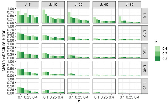
Figure 1. Estimation error for $\theta$ in simulated ZIPM data.

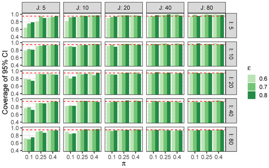
Figure 2. Nominal coverage of 95% confidence intervals for $\theta$ in simulated ZIPM data. Red dashed lines represent target coverage level of 0.95.

We observe that the methods derived in Section 4 yield accurate estimates of $\theta$ and well-calibrated confidence intervals. Figure 1 shows that mean absolute error decreases in I, J, $\pi$, and $ϵ$, and is generally small. The decrease in error as $\pi$ and $ϵ$ increase may be attributed to the corresponding increase in sample size for the less prevalent component and the decreasing amount of zero-inflation, respectively.

Figure 2 shows that coverage hovers close to 95% for most combinations of I, J, $\pi$, $\theta$. We observe that error is somewhat larger and coverage is somewhat inaccurate when $I,J\in \{5,10\}$. However, these inaccuracies are modest given the highly-limited data availability in these simulation scenarios.

5.2. Analysis of Frigatebird Nest Counts

We study ecological count data on frigatebirds in the Coral Sea Islands off the coast of Northeast Australia, as described in [1] (The specific data studied herein was provided via email with author G. Barry Baker). They obtained counts of frigatebird nests over 11 standardized sites across 4 separate time points.

This data is relevant to our study for two reasons: First, the ecological count data is zero-inflated. Of the 44 unique combinations of sites and time points in which data was collected, 7 had 0 nests (about 15.9%). Second, the frigatebird species has two subspecies, least (LFB) and greater (GFB). In the observed data, some nests were specified as LFB nests or GFB nests, but the majority were unidentified (Table 1). We analyze counts of only unidentified frigatebird nests, $N_{ij}$, by site i and time point j (Table 2).

Table 1. Counts of frigatebird nests by subspecies.

Frigatebird Subspecies	Nest Counts	Relative Proportion
Lesser	46	0.036
Greater	81	0.063
Unidentified	1158	0.901

Table 2. Total counts of 1158 unidentified frigatebird nests by site and time point.

Site	August 2007	September 2008	October 2009	August 2012
1	0	1	0	3
2	2	0	8	4
3	1	1	2	2
4	4	4	14	2
5	12	1	8	6
6	0	0	18	6
7	54	0	209	4
8	53	54	127	3
9	24	3	80	25
10	137	62	196	18
11	4	2	4	0

We applied our work from Section 4 to the unidentified nest counts in order to estimate the ratio $\theta \equiv \mu /\nu$, where $\mu$ and $\nu$ denote the expected numbers of nests per site for the less prevalent (Based on the numbers of nests that could be identified; see Table 1). LFB and more prevalent GFB, respectively. We set $t_i=1$ for each site i in the absence of additional information on each site (To assess the sensitivity of our results to this assumption, we have run an additional analysis in which $t_i$ is iteratively updated during the EM algorithm. We find estimates of $\theta$ are nearly unchanged; see Appendix C for details). During estimation the EM algorithm was run with 1000 random initializers.

Results appear in Table 3. We estimate that 25% of nests belong to LFB ($\widehat{\pi }=0.25$), 75% belong to GBF, and that 16% of observed nest counts are zero-inflated ($1-\widehat{ϵ}=0.16$). The EM algorithm yields the MLE $\widehat{\theta }=3.65$ for the ratio $\theta$; the 95% confidence interval for $\theta$ is (3.23, 4.08).

Table 3. ZIPM model MLEs to study unidentified frigatebird nests.

Parameter	$\mathit{\pi }$	$\mathit{ϵ}$	$\mathit{\mu }$	$\mathit{\nu }$	$\mathit{\theta }$ (95% CI)
Estimate	0.25	0.84	66.60	18.22	3.65 (3.23, 4.08)

6. Conclusions

In this paper, we studied the zero-inflated Poisson mixture (ZIPM) model in the frequentist setting. In addition to deriving an EM algorithm for point-estimation of model parameters, we stated an explicit formula for estimating standard errors of the MLEs. As a preliminary, we derived analogous results for the commonly-used, two-component Poisson mixture model. Although somewhat complex notationally, our formulae are straightforward to apply.

Our results were applied to real data on frigatebirds in the Coral Sea Islands off the coast of Northeastern Australia, where the ratio between two subspecies is of interest to ecologists. In this setting, knowledge of which species was more prevalent allows identifiability. We then used only unlabeled, zero-inflated nest count data to estimate (i) the relative abundance sites for each subspecies, (ii) the rate of zero-inflation, (iii) the mean numbers of nests per site for each subspecies, and (iv) the ratio of nests per site for each subspecies. We expect the ZIPM model to be useful in other ecological count data settings. Hence, our work provides straightforward ways for practitioners to estimate key parameters of interest.

Appendix C.1. Additional Results from Section 5.1

Table A1 and Table A2 display the results of Figure 1 and Figure 2, respectively, in tabular form.

Table A1. Mean absolute error in estimation of $\theta$ across varying values of I, J, $ϵ$, and $\pi$.

			J = 5			J = 10			J = 20			J = 40			J = 80
		$\mathbf{\pi }$	0.1	0.25	0.4	0.1	0.25	0.4	0.1	0.25	0.4	0.1	0.25	0.4	0.1	0.25	0.4
	$\mathbf{ϵ}$
$I=5$	0.6		0.82	0.70	0.55	0.94	0.39	0.30	0.75	0.29	0.19	0.39	0.14	0.12	0.44	0.09	0.08
	0.7		0.57	0.43	0.37	0.61	0.32	0.28	0.41	0.22	0.18	0.23	0.12	0.11	0.14	0.08	0.07
	0.8		0.54	0.52	0.42	0.47	0.27	0.23	0.31	0.21	0.15	0.18	0.11	0.10	0.15	0.08	0.07
$I=10$	0.6		0.55	0.34	0.33	0.38	0.24	0.18	0.27	0.13	0.12	0.15	0.08	0.08	0.10	0.06	0.06
	0.7		0.48	0.32	0.27	0.34	0.19	0.17	0.23	0.13	0.12	0.13	0.08	0.07	0.09	0.06	0.05
	0.8		0.43	0.27	0.26	0.32	0.22	0.15	0.24	0.11	0.10	0.12	0.08	0.07	0.07	0.05	0.05
$I=20$	0.6		0.49	0.28	0.21	0.33	0.15	0.12	0.20	0.09	0.08	0.10	0.06	0.06	0.06	0.05	0.04
	0.7		0.44	0.26	0.19	0.35	0.16	0.13	0.18	0.09	0.08	0.08	0.05	0.05	0.05	0.04	0.04
	0.8		0.45	0.28	0.18	0.30	0.13	0.11	0.16	0.08	0.07	0.07	0.05	0.05	0.05	0.04	0.04
$I=40$	0.6		0.47	0.24	0.15	0.26	0.12	0.09	0.14	0.06	0.06	0.07	0.04	0.04	0.05	0.03	0.03
	0.7		0.43	0.24	0.17	0.29	0.10	0.09	0.15	0.06	0.05	0.07	0.04	0.04	0.05	0.03	0.03
	0.8		0.48	0.22	0.14	0.23	0.09	0.08	0.09	0.05	0.04	0.06	0.04	0.04	0.04	0.03	0.02
$I=80$	0.6		0.45	0.20	0.11	0.17	0.11	0.06	0.08	0.05	0.04	0.04	0.03	0.03	0.03	0.02	0.02
	0.7		0.41	0.19	0.12	0.23	0.08	0.05	0.11	0.04	0.04	0.04	0.03	0.03	0.03	0.02	0.02
	0.8		0.38	0.18	0.10	0.23	0.09	0.05	0.11	0.04	0.03	0.04	0.03	0.03	0.03	0.02	0.02

Table A1. Mean absolute error in estimation of $\theta$ across varying values of I, J, $ϵ$, and $\pi$.

			J = 5			J = 10			J = 20			J = 40			J = 80
		$\mathbf{\pi }$	0.1	0.25	0.4	0.1	0.25	0.4	0.1	0.25	0.4	0.1	0.25	0.4	0.1	0.25	0.4
	$\mathbf{ϵ}$
$I=5$	0.6		0.82	0.70	0.55	0.94	0.39	0.30	0.75	0.29	0.19	0.39	0.14	0.12	0.44	0.09	0.08
	0.7		0.57	0.43	0.37	0.61	0.32	0.28	0.41	0.22	0.18	0.23	0.12	0.11	0.14	0.08	0.07
	0.8		0.54	0.52	0.42	0.47	0.27	0.23	0.31	0.21	0.15	0.18	0.11	0.10	0.15	0.08	0.07
$I=10$	0.6		0.55	0.34	0.33	0.38	0.24	0.18	0.27	0.13	0.12	0.15	0.08	0.08	0.10	0.06	0.06
	0.7		0.48	0.32	0.27	0.34	0.19	0.17	0.23	0.13	0.12	0.13	0.08	0.07	0.09	0.06	0.05
	0.8		0.43	0.27	0.26	0.32	0.22	0.15	0.24	0.11	0.10	0.12	0.08	0.07	0.07	0.05	0.05
$I=20$	0.6		0.49	0.28	0.21	0.33	0.15	0.12	0.20	0.09	0.08	0.10	0.06	0.06	0.06	0.05	0.04
	0.7		0.44	0.26	0.19	0.35	0.16	0.13	0.18	0.09	0.08	0.08	0.05	0.05	0.05	0.04	0.04
	0.8		0.45	0.28	0.18	0.30	0.13	0.11	0.16	0.08	0.07	0.07	0.05	0.05	0.05	0.04	0.04
$I=40$	0.6		0.47	0.24	0.15	0.26	0.12	0.09	0.14	0.06	0.06	0.07	0.04	0.04	0.05	0.03	0.03
	0.7		0.43	0.24	0.17	0.29	0.10	0.09	0.15	0.06	0.05	0.07	0.04	0.04	0.05	0.03	0.03
	0.8		0.48	0.22	0.14	0.23	0.09	0.08	0.09	0.05	0.04	0.06	0.04	0.04	0.04	0.03	0.02
$I=80$	0.6		0.45	0.20	0.11	0.17	0.11	0.06	0.08	0.05	0.04	0.04	0.03	0.03	0.03	0.02	0.02
	0.7		0.41	0.19	0.12	0.23	0.08	0.05	0.11	0.04	0.04	0.04	0.03	0.03	0.03	0.02	0.02
	0.8		0.38	0.18	0.10	0.23	0.09	0.05	0.11	0.04	0.03	0.04	0.03	0.03	0.03	0.02	0.02

Table A2. Nominal coverage of 95% confidence intervals for $\theta$ across varying values of I, J, $ϵ$, and $\pi$.

			J = 5			J = 10			J = 20			J = 40			J = 80
		$\mathbf{\pi }$	0.1	0.25	0.4	0.1	0.25	0.4	0.1	0.25	0.4	0.1	0.25	0.4	0.1	0.25	0.4
	$\mathbf{ϵ}$
$I=5$	0.6		0.65	0.81	0.92	0.82	0.93	0.97	0.90	0.98	0.97	0.95	0.98	0.99	0.94	0.98	1.00
	0.7		0.75	0.94	0.93	0.92	0.96	0.97	0.93	0.97	0.97	0.95	0.98	0.99	0.98	0.99	0.98
	0.8		0.79	0.90	0.96	0.93	0.96	0.97	0.94	0.97	0.96	0.97	1.00	0.96	0.96	0.98	0.98
$I=10$	0.6		0.79	0.91	0.93	0.89	0.94	0.96	0.91	0.96	0.98	0.95	0.98	0.97	0.98	0.95	0.98
	0.7		0.83	0.92	0.95	0.90	0.93	0.96	0.95	0.96	0.94	0.96	0.98	0.98	0.95	0.96	0.96
	0.8		0.81	0.94	0.94	0.89	0.94	0.96	0.89	0.96	0.95	0.96	0.94	0.96	0.98	0.96	0.96
$I=20$	0.6		0.80	0.92	0.95	0.88	0.97	0.98	0.92	0.95	0.96	0.96	0.94	0.92	0.96	0.94	0.94
	0.7		0.78	0.92	0.91	0.80	0.91	0.89	0.91	0.94	0.96	0.94	0.95	0.95	0.96	0.95	0.96
	0.8		0.74	0.91	0.90	0.86	0.93	0.95	0.90	0.96	0.93	0.97	0.96	0.94	0.94	0.94	0.96
$I=40$	0.6		0.77	0.90	0.93	0.83	0.95	0.96	0.91	0.95	0.93	0.91	0.95	0.94	0.94	0.94	0.98
	0.7		0.79	0.91	0.95	0.84	0.96	0.95	0.93	0.96	0.97	0.96	0.93	0.95	0.95	0.94	0.98
	0.8		0.73	0.89	0.94	0.83	0.96	0.93	0.95	0.98	0.96	0.95	0.94	0.92	0.92	0.94	0.95
$I=80$	0.6		0.72	0.90	0.94	0.90	0.93	0.95	0.97	0.95	0.95	0.95	0.97	0.92	0.96	0.93	0.94
	0.7		0.70	0.91	0.94	0.84	0.95	0.96	0.92	0.94	0.96	0.94	0.94	0.94	0.93	0.94	0.96
	0.8		0.75	0.87	0.94	0.86	0.96	0.97	0.93	0.95	0.96	0.95	0.94	0.93	0.94	0.94	0.94

Table A2. Nominal coverage of 95% confidence intervals for $\theta$ across varying values of I, J, $ϵ$, and $\pi$.

			J = 5			J = 10			J = 20			J = 40			J = 80
		$\mathbf{\pi }$	0.1	0.25	0.4	0.1	0.25	0.4	0.1	0.25	0.4	0.1	0.25	0.4	0.1	0.25	0.4
	$\mathbf{ϵ}$
$I=5$	0.6		0.65	0.81	0.92	0.82	0.93	0.97	0.90	0.98	0.97	0.95	0.98	0.99	0.94	0.98	1.00
	0.7		0.75	0.94	0.93	0.92	0.96	0.97	0.93	0.97	0.97	0.95	0.98	0.99	0.98	0.99	0.98
	0.8		0.79	0.90	0.96	0.93	0.96	0.97	0.94	0.97	0.96	0.97	1.00	0.96	0.96	0.98	0.98
$I=10$	0.6		0.79	0.91	0.93	0.89	0.94	0.96	0.91	0.96	0.98	0.95	0.98	0.97	0.98	0.95	0.98
	0.7		0.83	0.92	0.95	0.90	0.93	0.96	0.95	0.96	0.94	0.96	0.98	0.98	0.95	0.96	0.96
	0.8		0.81	0.94	0.94	0.89	0.94	0.96	0.89	0.96	0.95	0.96	0.94	0.96	0.98	0.96	0.96
$I=20$	0.6		0.80	0.92	0.95	0.88	0.97	0.98	0.92	0.95	0.96	0.96	0.94	0.92	0.96	0.94	0.94
	0.7		0.78	0.92	0.91	0.80	0.91	0.89	0.91	0.94	0.96	0.94	0.95	0.95	0.96	0.95	0.96
	0.8		0.74	0.91	0.90	0.86	0.93	0.95	0.90	0.96	0.93	0.97	0.96	0.94	0.94	0.94	0.96
$I=40$	0.6		0.77	0.90	0.93	0.83	0.95	0.96	0.91	0.95	0.93	0.91	0.95	0.94	0.94	0.94	0.98
	0.7		0.79	0.91	0.95	0.84	0.96	0.95	0.93	0.96	0.97	0.96	0.93	0.95	0.95	0.94	0.98
	0.8		0.73	0.89	0.94	0.83	0.96	0.93	0.95	0.98	0.96	0.95	0.94	0.92	0.92	0.94	0.95
$I=80$	0.6		0.72	0.90	0.94	0.90	0.93	0.95	0.97	0.95	0.95	0.95	0.97	0.92	0.96	0.93	0.94
	0.7		0.70	0.91	0.94	0.84	0.95	0.96	0.92	0.94	0.96	0.94	0.94	0.94	0.93	0.94	0.96
	0.8		0.75	0.87	0.94	0.86	0.96	0.97	0.93	0.95	0.96	0.95	0.94	0.93	0.94	0.94	0.94

Appendix C.2. Additional Results from Section 5.2

To assess the sensitivity of our results to the assumption that $t_i=1$ for each site $i=1,\dots ,11$, we ran a sensitivity analysis in which $t_i$ was iteratively updated during the E-step of the proposed EM algorithm. Specifically, we updated $t_i$ by maximizing (9) conditional on current estimates of $\widehat{y}$, $\widehat{z}$, $\widehat{\mu }$, and $\widehat{\nu }$ at any given step of the algorithm. After estimation, estimates of $t_i$ were treated as fixed and known.

Results under this sensitivity analysis appear in Table A3. We notice that estimates of $\theta$, $\pi$, and $ϵ$ are remarkably similar, while estimates of $\mu$ and $\nu$ are each changed by the same scale factor. Thus, we observe that our results for the parameter of interest, $\theta$, are not sensitive to our choice of $t_i$ in this case.

Table A3. Sensitivity analysis results when estimating $t_i$ in frigatebird analysis.

Parameter	$\mathit{\pi }$	$\mathit{ϵ}$	$\mathit{\mu }$	$\mathit{\nu }$	$\mathit{\theta }$ (95% CI)
Estimate	0.25	0.88	50.55	13.84	3.65 (3.22, 4.08)
Site (i)	1	2	3	4	5	6	7	8	9	10	11
${\widehat{t}}_i$	0.104	0.166	0.065	0.261	0.293	0.366	3.413	2.574	1.434	4.485	0.116

Table A3. Sensitivity analysis results when estimating $t_i$ in frigatebird analysis.

Parameter	$\mathit{\pi }$	$\mathit{ϵ}$	$\mathit{\mu }$	$\mathit{\nu }$	$\mathit{\theta }$ (95% CI)
Estimate	0.25	0.88	50.55	13.84	3.65 (3.22, 4.08)
Site (i)	1	2	3	4	5	6	7	8	9	10	11
${\widehat{t}}_i$	0.104	0.166	0.065	0.261	0.293	0.366	3.413	2.574	1.434	4.485	0.116

References

- Baker, G.B.; Holdsworth, M. Seabird monitoring study at Coringa Herald National Nature Reserve 2012; Report Prepared for Department of Sustainability, Environment, Water, Populations and Communities; Latitude 42 Environmental Consultants Pty Ltd.: Kettering, TAS, Australia, 2013. [Google Scholar]
- Bouveyron; Celeux, C.G.; Murphy, T.B.; Raftery, A.E. Model-Based Clustering and Classification for Data Science: With Applications in R; Cambridge University Press: Cambridge, UK, 2019. [Google Scholar]
- Lindsay, B.G. Mixture Models: Theory, Geometry, and Applications; Institute for Mathematical Statistics: Hayward, CA, USA, 1995. [Google Scholar]
- McLachlan, G.J.; Peel, D. Finite Mixture Models; Wiley: New York, NY, USA, 2000. [Google Scholar]
- Martin, T.G.; Wintle, B.A.; Rhodes, J.R.; Kuhnert, P.M.; Field, S.A.; Low-Choy, S.J.; Tyre, A.J.; Possingham, H.P. Zero tolerance ecology: Improving ecological inference by modelling the source of zero observations. Ecol. Lett. 2005, 8, 1235–1246. [Google Scholar] [CrossRef] [PubMed]
- Lambert, D. Zero-inflated Poisson regression, with an application to defects in manufacturing. Technometrics 1992, 34, 1–14. [Google Scholar] [CrossRef]
- Lim, H.K.; Li, W.K.; Philip, L.H. Zero-inflated Poisson regression mixture model. Comput. Stat. Data Anal. 2014, 71, 151–158. [Google Scholar] [CrossRef]
- Long, D.L.; Preisser, J.S.; Herring, A.H.; Golin, C.E. A marginalized zero-inflated Poisson regression model with overall exposure effects. Stat. Med. 2014, 33, 5151–5165. [Google Scholar] [CrossRef] [PubMed]
- Jamshidian, M.; Jennrich, R.I. Standard errors for EM estimation. J. R. Stat. Soc. Ser. B 2000, 62, 257–270. [Google Scholar] [CrossRef]
- Aitken, M.; Rubin, D.B. Estimation and hypothesis testing in finite mixture models. J. R. Stat. Soc. Ser. B 1985, 47, 67–75. [Google Scholar] [CrossRef]
- McLachlan, G.J.; Krishnan, T. The EM Algorithms and its Extensions, 2nd ed.; Wiley: New York, NY, USA, 2008. [Google Scholar]
- Hoadley, B. Asymptotic properties of maximum likelihood estimators for the independent not identically distributed case. Ann. Math. Stat. 1971, 42, 1977–1991. [Google Scholar] [CrossRef]
- Efron, B.; Hinkley, D.V. Assessing the accuracy of the maximum likelihood estimator: Observed versus expected Fisher information. Biometrika 1978, 65, 457–482. [Google Scholar] [CrossRef]
- Louis, T. Finding the observed information matrix when using the EM Algorithm. J. R. Stat. Soc. Ser. B 1982, 44, 226–233. [Google Scholar] [CrossRef]
- Johnson, N.L.; Kemp, A.W.; Kotz, S. Univariate Discrete Distributions, 3rd ed.; Wiley-Interscience: Hoboken, NJ, USA, 2005. [Google Scholar]
Disclaimer/Publisher’s Note: The statements, opinions and data contained in all publications are solely those of the individual author(s) and contributor(s) and not of MDPI and/or the editor(s). MDPI and/or the editor(s) disclaim responsibility for any injury to people or property resulting from any ideas, methods, instructions or products referred to in the content. |
© 2025 by the authors. Licensee MDPI, Basel, Switzerland. This article is an open access article distributed under the terms and conditions of the Creative Commons Attribution (CC BY) license (https://creativecommons.org/licenses/by/4.0/).