A Novel Flexible Class of Intervened Poisson Distribution by Lagrangian Approach

Abstract

The zero-truncated Poisson distribution (ZTPD) generates a statistical model that could be appropriate when observations begin once at least one event occurs. The intervened Poisson distribution (IPD) is a substitute for the ZTPD, in which some intervention processes may change the mean of the rare events. These two zero-truncated distributions exhibit underdispersion (i.e., their variance is less than their mean). In this research, we offer an alternative solution for dealing with intervention problems by proposing a generalization of the IPD by a Lagrangian approach called the Lagrangian intervened Poisson distribution (LIPD), which in fact generalizes both the ZTPD and the IPD. As a notable feature, it has the ability to analyze both overdispersed and underdispersed datasets. In addition, the LIPD has a closed-form expression of all of its statistical characteristics, as well as an increasing, decreasing, bathtub-shaped, and upside-down bathtub-shaped hazard rate function. A consequent part is devoted to its statistical application. The maximum likelihood estimation method is considered, and the effectiveness of the estimates is demonstrated through a simulated study. To evaluate the significance of the new parameter in the LIPD, a generalized likelihood ratio test is performed. Subsequently, we present a new count regression model that is suitable for both overdispersed and underdispersed datasets using the mean-parametrized form of the LIPD. Additionally, the LIPD’s relevance and application are shown using real-world datasets.

1. Introduction

In many real-world circumstances, the researcher is unable to see the whole distribution of counts in an experiment. The ZTPD was applied in [1] to explain a chance process in which the observation apparatus only activates when at least one event occurs. A new kind of distribution that incorporates the concept of intervention has received much attention in the literature. The intervened Poisson distribution (IPD) was first developed in [2] as an alternative to the ZTPD, in which some intervention process alters the mean of the rare events. It would be interesting to look into the effects of such a decision on the queuing mechanism. For instance, a store manager might decide to offer more assistance at a service counter in order to increase the service rate. Healthcare professionals may use a range of preventive strategies in epidemiological research, such as in cholera instances. In addition to reliability analysis, queuing problems, and epidemiological research, the IPD has also been applied in other contexts (see [3,4,5]). In order to examine scenarios involving two interventions, the authors in [6] proposed and studied a modified version of the IPD, which they called the modified IPD. For prevalence reduction, the authors in [7] presented an alternative to the IPD. According to [2], one important limitation of the IPD is that it is underdispersed. There is no reason to assume that data generated by any of the aforementioned applications will necessarily share this feature. To alleviate this issue, the authors in [8] introduced a generalization of the IPD, namely the intervened generalized Poisson distribution (IGPD), which accommodates both underdispersed and overdispersed (i.e., its variance is greater than its mean) natures. However, its ability to fit some of the intervention problems is not sufficient (see [8]), which indicates that the literature still has a gap in how to deal with intervention problems. By suggesting a generalization of the IPD using a well-known Lagrangian approach and calling it the LIPD, we hope to do more to close this gap through this endeavor.

Lagrangian expansions, which were first described in [9], are the parent category of Lagrangian distributions. The discrete Lagrangian family (DLF), a large and significant class that includes many probability distributions, was introduced in [10,11]. In [11], the authors showed that, under certain conditions, all the discrete Lagrangian distributions converge to the normal and inverse Gaussian distributions. Based on these former works, the DLF has found many applications in probability and statistics; some of its recent developments are presented below. The Lagrangian Katz family was developed in [12]. The authors in [13] examined the use of Lagrangian probability distributions for the resolution of inferential issues in random mapping theory. The authors in [14] used Lagrangian probability models to create the generalized Poisson gamma dependence model. Using Lagrangian probability distributions, the authors in [15] exploited collisional turbulent fluid–particle flows. Furthermore, the authors in [16] discussed the methods for generating different classes of Lagrangian probability distributions. Our team was very impressed by the competency of the distributions proposed based on the Lagrangian method, and as a result, we proposed the Lagrangian version of ZTPD through the work published in [17]. Furthermore, the authors in [18] concentrated on the Lagrangian approach’s construction of the zero-truncated binomial distribution (ZTBD) and explained how effective it was in comparison to other zero-truncated distributions. The aforementioned relevance once more compelled us to develop solutions to intervention problems using a Lagrangian approach, which we dub the LIPD. The LIPD model was developed primarily for the following reasons: (i) to offer a flexible generalization of the parent IPD, as well as the ZTPD; (ii) to accommodate various shapes of the hazard rate function (HRF), including increasing, decreasing, bathtub, and upside-down bathtub shapes; (iii) to deal with underdispersed and overdispersed real-world datasets; and (iv) to specifically apply the real-world datasets generated from the intervention situations.

On the other hand, currently, regression models for count data are gaining much popularity. In some real-world scenarios, however, the mechanism will only activate if at least one event occurs. The number of foreign conflicts, daily mishaps, industrial casualties, and so on, are all examples. As detailed in [19], counting outcomes directly with a normal linear regression model leads to inefficient, inconsistent, and biased estimation in many cases. The zero-truncated Poisson regression model (ZTPRM) is used to analyze positive count data because it is more accurate than the classical Poisson regression model for such data. The authors in [20] recently created an alternative to the ZTPRM, called the intervened Poisson regression model (IPRM). The Lagrangian intervened Poisson regression model (LIPRM), which is an alternative to both the ZTPRM and the IPRM, is presented in this study. The motivation behind introducing the LIPRM includes its applicability for situations where the modeled data exclude zero counts, dealing with intervention problems, and its appropriateness for both underdispersed and overdispersed count datasets.

An overview of the remaining study sections is provided below: Section 2 gives a quick overview of the Lagrangian expansion and the IPD. Some important Lagrangian probability models are discussed in Section 3. In Section 4, the LIPD and its statistical features are explored. In Section 5, the maximum likelihood (ML) estimation approach is developed. A generalized likelihood ratio test is elaborated in Section 6 to examine the importance of an extra parameter of the LIPD. The simulation results of the suggested estimating method are included in Section 7. In Section 8, the LIPRM is explained. Section 9 provides empirical examples of the recommended LIPD and LIPRM. Finally, Section 10 provides the conclusion of the article.

2. Some Preliminaries

For the development of the LIPD, we present some fundamental findings in this section.

2.1. Intervened Poisson Distribution

To begin, we consider the definition of the ZTPD. Let $X_1$ be a random variable (RV) representing the number of occurrences of some rare event, and let us assume that the event $X_1=0$ is not observable. Then, it is plausible that $X_1$ follows the ZTPD with the following probability mass function (PMF):

$$g\left(x_1\right)=\frac{{\lambda }^{x_1}}{x_1!(e^{\lambda }-1)},$$

with $\lambda >0$, for those values of $x_1$ on the positive integers, and zero elsewhere.

Following the generation of $X_1$, it is presumable that some intervention transforms $\lambda$ into $\lambda \rho$, where $\rho \ge 0$. Let $X_2$ be an RV representing the number of instances of the rare event that occurred after the intervention. It has a Poisson RV with a mean of $\lambda \rho$ and is statistically independent of $X_1$. Assuming that our observational device only has a record of the RV $X=X_1+X_2$, the distribution of the total number of rare events that occurred can be assimilated to an IPD with parameters $\lambda$ and $\rho$. Then, the PMF of X is presented below.

Definition 1.

An RV X is said to follow the IPD, if its PMF is defined as:

$$\mathrm{Pr}(X=x)=\frac{\left[{(1+\rho )}^x-{\rho }^x\right]{\lambda }^x}{e^{\lambda \rho }(e^{\lambda }-1)x!},x=1,2,3,\dots ,$$

(1)

with $\lambda >0$ and $\rho \ge 0$.

The mean and variance of an RV X that follows the IPD are, respectively, given by

$$\mathrm{E}\left(X\right)=\lambda \left(\rho +1+{(e^{\lambda }-1)}^{-1}\right)$$

and

$$\mathrm{Var}\left(X\right)=\mathrm{E}\left(X\right)-e^{\lambda }{\left(\frac{\lambda }{e^{\lambda }-1}\right)}^2.$$

Remark 1.

The IPD is underdispersed, for all values of λ and ρ (see [2]).

2.2. Lagrange Expansion

In order to present the LIPD, some mathematical background on the Lagrangian expansion is required.

Let $h_1\left(z\right)$ and $h_2\left(z\right)$ be two analytic and successively differentiable functions with respect to z defined on the interval $[-1,1]$ such that $h_1\left(1\right)=h_2\left(1\right)=1$, $h_1\left(0\right)\ne 0$, and $h_2\left(0\right)\ge 0$. Inverting the Lagrange transformation yields the following series expansion:

$$\frac{h_2\left(z\right)}{1-\frac{z{h}_1^{{}^{\prime }}\left(z\right)}{h_1\left(z\right)}}=\sum _{j=0}^{\infty }{c}_j{u}^j,$$

(2)

where $z=u{h}_1\left(z\right)$, $c_0=h_2\left(0\right)$ and $c_j=\frac{1}{j!}\left\{D^j\left[{\left(h_1\left(z\right)\right)}^j{h}_2\left(z\right)\right]\right\}{|}_{z=0}$, with $D^j$= $\frac{{\partial }^j}{\partial z^j}$, and $h_1^{\prime }\left(z\right)=\frac{\partial h_1\left(z\right)}{\partial z}$.

The details can be found in [21]. Moreover, if

$$0<h_1^{\prime }\left(1\right)<1\mathrm{and}\left\{D^j\left[{\left(h_1\left(z\right)\right)}^j{h}_2\left(z\right)\right]\right\}{|}_{z=0}\ge 0,j\ge 0,$$

(3)

the Lagrange expansion (2) defines the DLF. In light of this, an RV X belonging to the DLF has the PMF shown below:

$$\mathrm{Pr}(X=x)=\frac{\left(1-h_1^{\prime }\left(1\right)\right)\left\{D^x\left[{\left(h_1\left(z\right)\right)}^x{h}_2\left(z\right)\right]\right\}{|}_{z=0}}{x!},x=0,1,2,\dots$$

(4)

The associated probability-generating function (PGF) is generated by

$$H\left(u\right)=\frac{(1-h_1^{\prime }\left(z\right))h_2\left(z\right)}{1-\frac{z{h}_1^{\prime }\left(z\right)}{h_1\left(z\right)}},$$

(5)

where $z=u{h}_1\left(z\right).$ In order to learn more about this special class, see [21,22].

3. Some Important Members of Discrete Lagrangian Family

Many DLF members can be generated by taking the following exponential function:

$$\begin{array}{c}\hfill h_1\left(z\right)=e^{\mu (z-1)},\end{array}$$

(6)

with $0<\mu <1$ and various choices of the functions for $h_2\left(z\right)$ in (4). Some of them are discussed below:

3.1. Sudha Lagrangian Distribution

Let us take $h_1\left(z\right)$ as in (6) and $h_2\left(z\right)=z$. Based on (4), the PMF of the considered distribution can be derived as:

$$\begin{array}{cc}\hfill g_1\left(x\right)& =(1-\mu )\frac{D^x\left[e^{\mu x(z-1)}z\right]{|}_{z=0}}{x!}\hfill \\ \hfill & =\frac{(1-\mu )e^{-x\mu }{\left(x\mu \right)}^{x-1}}{(x-1)!},x=1,2,3\dots ,\hfill \end{array}$$

which is the PMF of the Sudha Lagrangian distribution (see [23]).

3.2. Weighted Delta Poisson Distribution

More generally, if we take $h_1\left(z\right)$ as in (6) and $h_2\left(z\right)=z^n$ with $n\ge 1$, the PMF based on (4) is obtained as:

$$\begin{array}{cc}\hfill g_2\left(x\right)& =(1-\mu )\frac{D^x\left[e^{\mu x(z-1)}{z}^n\right]{|}_{z=0}}{x!}\hfill \\ \hfill & =(1-\mu )\frac{e^{-x\mu }{\left(x\mu \right)}^{x-n}}{(x-n)!},x=n,n+1,n+2\dots ,\hfill \end{array}$$

which corresponds to the PMF of the weighted delta Poisson distribution (see [23]).

3.3. Linear Function Poisson Distribution

If we take $h_1\left(z\right)$ as in (6) and $h_2\left(z\right)=e^{\lambda (z-1)}$ with $\lambda >0$, the PMF based on (4) is obtained as:

$$\begin{array}{cc}\hfill g_3\left(x\right)& =(1-\mu )\frac{D^x\left[e^{\mu x(z-1)}{e}^{\lambda (z-1)}\right]{|}_{z=0}}{x!}\hfill \\ \hfill & =\frac{(1-\mu ){(\lambda +x\mu )}^x{e}^{-\lambda -x\mu }}{x!},x=0,1,2,\dots ,\hfill \end{array}$$

which corresponds to the PMF of the linear function Poisson distribution (see [23]).

3.4. Logarithmic Poisson Distribution

If we take $h_1\left(z\right)$ as in (6) and $h_2\left(z\right)=\frac{log(1-pz)}{log(1-p)}$ with $0<p<1$, the PMF based on (4) is obtained as:

$$\begin{array}{cc}\hfill g_4\left(x\right)& =(1-\mu )\frac{D^x\left[e^{\mu x(z-1)}\frac{log(1-pz)}{(log(1-p))}\right]{|}_{z=0}}{x!}\hfill \\ \hfill & =\frac{(1-\mu )}{-log(1-p)}{e}^{-\mu x}{\left(\mu x\right)}^x\sum _{k=1}^x\frac{{\left(\frac{p}{\mu x}\right)}^k}{k(x-k)!},x=0,1,2,\dots ,\hfill \end{array}$$

which corresponds to the PMF of the logarithmic Poisson distribution (see [23]).

Given the applications of the DLF created with $h_1\left(z\right)=e^{\mu (z-1)}$ and modulating $h_2\left(z\right)$, it is worthwhile to investigate other horizon distributions. This served as the foundation for the amended study distribution, which is displayed below.

4. Lagrangian Intervened Poisson Distribution

In this section, the definition of the new distribution and some of its primary characteristics are described.

Suppose

$$h_1\left(z\right)=e^{\mu (z-1)}\mathrm{and}{h}_2\left(z\right)=\frac{(e^{z\lambda }-1)e^{\lambda \rho (z-1)}}{e^{\lambda }-1},$$

(7)

so that $h_2\left(z\right)$ is the PGF of the IPD (see [2]) with $\lambda >0$ and $\rho \ge 0$.

The corresponding analytic functions given in (7) satisfy the conditions given in Section 2.2, are completely new in this context, and benefit from interesting functionalities for modeling purposes. Then, under the following transformation: $u=\frac{z}{h_1\left(z\right)}=\frac{z}{e^{\mu (z-1)}}$, we have

$$\begin{array}{cc}\hfill \left\{D^j\left({\left(h_1\left(z\right)\right)}^j{h}_2\left(z\right)\right)\right\}{|}_{z=0}& =\left\{D^j\left(e^{\mu j(z-1)}\frac{(e^{z\lambda }-1)e^{\lambda \rho (z-1)}}{e^{\lambda }-1}\right)\right\}{|}_{z=0}\hfill \\ \hfill & =\frac{e^{-\left(\lambda \rho +\mu j\right)}}{e^{\lambda }-1}\left\{{\left(j\mu +\lambda +\lambda \rho \right)}^j-{\left(j\mu +\lambda \rho \right)}^j\right\}.\hfill \end{array}$$

From the above expression, it is clear that the condition given in (3) is satisfied. Then, using (4), the corresponding PMF of the LIPD can be derived as:

$$\begin{array}{cc}\hfill g\left(x\right)=& \frac{(1-\mu )}{x!}{D}^x\left[e^{\mu x(z-1)}\frac{(e^{z\lambda }-1)e^{\lambda \rho (z-1)}}{e^{\lambda }-1}\right]{|}_{z=0}\hfill \\ \hfill & =\frac{(1-\mu )e^{-(\lambda \rho +\mu x)}}{(e^{\lambda }-1)x!}\left\{{(x\mu +\lambda +\lambda \rho )}^x-{(x\mu +\lambda \rho )}^x\right\}.\hfill \end{array}$$

We formalize this definition below.

Definition 2.

A RV X is said to follow the LIPD, if its PMF has the following form:

$$g\left(x\right)=\frac{(1-\mu )e^{-(\lambda \rho +\mu x)}}{(e^{\lambda }-1)x!}\left\{{(x\mu +\lambda +\lambda \rho )}^x-{(x\mu +\lambda \rho )}^x\right\},x=1,2,3,\dots ,$$

(8)

where $\lambda >0$, $\rho \ge 0$, and $0<\mu <1$.

A distribution with the PMF given in (8) will be sometimes denoted as LIPD ($\lambda ,\mu ,\rho$). In addition, the RV X that will appear is supposed to follow this distribution. Some special cases are described below:

• For $\mu \to 0$, the LIPD ($\lambda ,\mu ,\rho$) reduces to the IPD.
• For $\mu \to 0$ and $\rho =0$, the LIPD ($\lambda ,\mu ,\rho$) reduces to the ZTPD.

Figure 1, Figure 2 and Figure 3 display the graphical representation of the PMF of the LIPD for different parameter values of $\lambda$, $\mu$, and $\rho$, respectively.

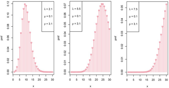
Figure 1. Various shapes of the PMF of the LIPD when $\lambda$ increases.

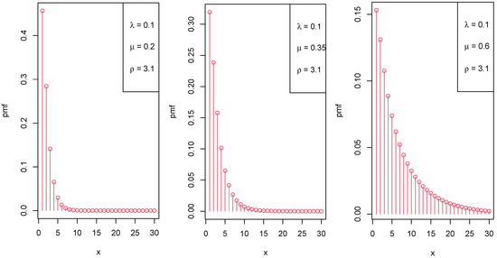
Figure 2. Various shapes of the PMF of the LIPD when $\mu$ increases.

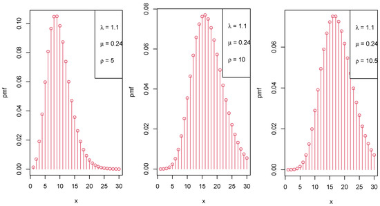
Figure 3. Various shapes of the PMF of the LIPD when $\rho$ increases.

The HRF of the LIPD is obtained by substituting the PMF in the following equation:

$$\begin{array}{c}\hfill h\left(x\right)=\mathrm{Pr}(X=x|X\ge x)=\frac{g\left(x\right)}{{\sum }_{k=x}^{\infty }g\left(k\right)}.\end{array}$$

(9)

It is obvious from (9) that finding the closed-form expression of the HRF is difficult. To identify the diverse forms of the HRF, we draw the corresponding graph in Figure 4.

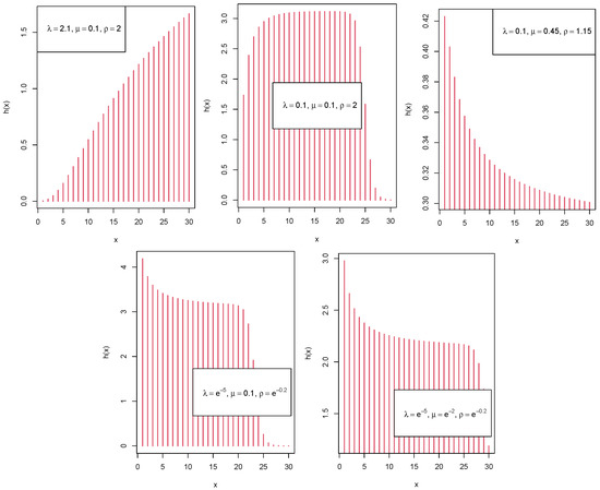
Figure 4. Plots of the HRF of the LIPD distribution.

Figure 4 shows that the LIPD has an increasing, decreasing, bathtub, and upside-down bathtub-shaped HRF.

Proposition 1.

Let X be an RV following the LIPD. Then, the mode of X, denoted by $x_m$, exists and lies in the following case:

$$\frac{\varrho (x_m+1)}{\varrho \left(x_m\right)}-e^{\mu }\le x_m{e}^{\mu }\le \frac{\varrho \left(x_m\right)}{\varrho (x_m-1)},$$

(10)

$where$$\varrho \left(x_m\right)={(\mu x_m+\lambda +\lambda \rho )}^{x_m}-{(\mu x_m+\lambda \rho )}^{x_m}$.

Proof. 

According to the definition of a mode in a discrete distribution setting, we must find the integer $x=x_m$ for which $g\left(x\right)$ has the greatest value. That is, we aim to solve the following inequalities: $g\left(x\right)\ge g(x-1)$ and $g\left(x\right)\ge g(x+1)$, where $g\left(x\right)$ can also be written as:

$$g\left(x\right)=\frac{1-\mu }{e^{\lambda }-1}\frac{e^{-\mu x-\lambda \rho }\varrho \left(x\right)}{x!},$$

(11)

where $\varrho \left(x\right)={(\lambda \rho +\lambda +\mu x)}^x-{(\lambda \rho +\mu x)}^x$.

Obviously, $g\left(x\right)\ge g(x-1)$ implies that

$$\frac{\varrho \left(x\right)}{\varrho (x-1)}\ge x{e}^{\mu }.$$

(12)

Furthermore, $g\left(x\right)\ge g(x+1)$ implies that

$$\frac{\varrho (x+1)}{\varrho \left(x\right)}\le (x+1)e^{\mu }.$$

(13)

By combining (12) and (13), we obtain (10).    □

Proposition 2.

The PGF of an RV X following the LIPD is expressed as

$$H\left(u\right)=\mathrm{E}\left(u^X\right)=\frac{(1-\mu )(e^{z\lambda }-1)e^{\lambda \rho (z-1)}}{(e^{\lambda }-1)(1-\mu z)},$$

(14)

where $z=u{e}^{\mu (z-1)}$ with $\mu z<1$.

Proof. 

By virtue of (5), we immediately get

$$\begin{array}{cc}\hfill H\left(u\right)& =\frac{(1-h_1^{\prime }\left(1\right))h_2\left(z\right)}{1-\frac{z{h}_1^{\prime }\left(z\right)}{h_1\left(z\right)}}=\frac{(1-\mu )(e^{z\lambda }-1)e^{\lambda \rho (z-1)}}{(e^{\lambda }-1)(1-\mu z)},\hfill \end{array}$$

where $z=u{e}^{\mu (z-1)}$. Thus, the proof is obtained.    □

Corollary 1.

The moment-generating function (MGF) of an RV X following the LIPD is obtained by putting $z=e^s$ and $u=e^k$ in (14), and we obtain

$$\mathrm{M}\left(k\right)=\mathrm{E}\left(e^{kX}\right)=\frac{(1-\mu )(e^{\lambda e^s}-1)e^{\lambda \rho (e^s-1)}}{(e^{\lambda }-1)(1-\mu e^s)},$$

where $s=k+\mu (e^s-1)$ with $s<-log\left(\mu \right)$.

Corollary 2.

The cumulant-generating function (CGF) of an RV X following the LIPD becomes

$$\mathrm{C}\left(k\right)=log\left[\mathrm{M}\left(k\right)\right]=log\left\{\frac{(1-\mu )(e^{\lambda e^s}-1)e^{\lambda \rho (e^s-1)}}{(e^{\lambda }-1)(1-\mu e^s)}\right\},$$

where $s=k+\mu (e^s-1)$ with $s<-log\left(\mu \right)$.

Proposition 3.

Let $X_1,X_2,\dots ,X_n$ be n independently and identically distributed (IID) RVs following the LIPD. Then, the distribution of the sample sum $V={\sum }_{k=1}^n{X}_k$ has the following PGF:

$$\begin{array}{c}\hfill \Psi \left(u\right)=\frac{{(1-\mu )}^n{(e^{z\lambda }-1)}^n{e}^{n\lambda \rho (z-1)}}{{(e^{\lambda }-1)}^n{(1-z\mu )}^n},\end{array}$$

where $z=u{e}^{\mu (z-1)}$.

Proof. 

Based on the PGF of the LIPD given in (14), the PGF of the RV V becomes

$$\begin{array}{cc}\hfill \Psi \left(u\right)& =\mathrm{E}\left(u^V\right)={\left[H\left(u\right)\right]}^n=\frac{{(1-\mu )}^n{(e^{z\lambda }-1)}^n{e}^{n\lambda \rho (z-1)}}{{(e^{\lambda }-1)}^n{(1-\mu z)}^n}.\hfill \end{array}$$

This completes the proof.    □

Proposition 4.

For any integer $r\ge 1$, the rth factorial moment of an RV X following the LIPD is given by

$$\begin{array}{cc}\hfill & {\mu }_{\left[r\right]}=\mathrm{E}[X(X-1)\dots (X-r+1)]\hfill \\ \hfill & =\left\{\frac{D^r\left((e^{z\lambda }-1)e^{\lambda \rho (z-1)}\right)}{e^{\lambda }-1}+\mu \frac{{\sum }_{i=1}^r(r-i+1){\mu }_{[r-i]}{D}^i\left(u{e}^{\mu (z-1)}\right)}{1-\mu }\right\}{|}_{u=z=1},\hfill \end{array}$$

(15)

where $z=u{e}^{\mu (z-1)}$.

Proof. 

By definition, the rth factorial moment is obtained by successively differentiating $H\left(u\right)$ given in (5) in r times with respect to u and by putting $u=z=1$. Thus, it is given by

$$H\left(u\right)=\frac{(1-h_1^{\prime }\left(1\right))h_2\left(z\right)}{1-u{h}_1^{\prime }\left(z\right)},$$

implying that

$$(1-u{h}_1^{\prime }\left(z\right))H\left(u\right)=(1-h_1^{\prime }\left(1\right))h_2\left(z\right).$$

Taking the first derivative with respect to u on both sides, we obtain

$$H\left(u\right)D^1(1-u{h}_1^{\prime }\left(z\right))+H^{\prime }\left(u\right)(1-u{h}_1^{\prime }\left(z\right))=(1-h_1^{\prime }\left(1\right))D^1{h}_2\left(z\right).$$

(16)

Again, by taking the derivative of (16) with respect to u on both sides, we obtain

$$\begin{array}{cc}\hfill & H\left(u\right)D^2(1-u{h}_1^{\prime }\left(z\right))+2D^2(1-u{h}_1^{\prime }\left(z\right))H^{\prime }\left(u\right)+(1-u{h}_1^{\prime }\left(z\right))H^{″}\left(u\right)\hfill \\ \hfill & =(1-h_1^{\prime }\left(1\right))D^2{h}_2\left(z\right).\hfill \end{array}$$

Proceeding like this, we obtain that the rth derivative is of the following form:

$$D^r\left(H\left(u\right)\right)=\frac{(1-h_1^{\prime }\left(1\right))D^r\left(h_2\left(z\right)\right)-{\sum }_{i=1}^r(r-i+1)D^i(1-u{h}_1^{\prime }\left(z\right))D^{r-i}\left(H\left(u\right)\right)}{1-u{h}_1^{\prime }\left(z\right)}$$

(17)

Substituting $h_1\left(z\right)=e^{\mu (z-1)}$, $h_2\left(z\right)=\frac{(e^{z\lambda }-1)e^{\lambda \rho (z-1)}}{e^{\lambda }-1}$, and $z=u=1$ in (17), we obtain (15).    □

Proposition 5.

The mean (${\mu }_1^{{}^{\prime }}$) and variance (${\sigma }^2$) of an RV X following the LIPD are

$${\mu }_1^{{}^{\prime }}=\mathrm{E}\left(X\right)=\frac{\lambda }{(1-\mu )(1-e^{-\lambda })}+\frac{\lambda \rho (1-\mu )+\mu }{{(1-\mu )}^2}$$

and

$$\begin{array}{cc}\hfill {\sigma }^2=\mathrm{Var}\left(X\right)=& \frac{\mu (\mu +1)}{{(1-\mu )}^4}+\frac{\left(e^{\lambda }{(\lambda +\lambda \rho )}^2-{\lambda }^2{\rho }^2\right)(1-\mu )+\left(e^{\lambda }(\lambda +\lambda \rho )-\lambda \rho \right)}{(e^{\lambda }-1){(1-\mu )}^3}\hfill \\ & -\frac{{\left\{e^{\lambda }(\lambda +\lambda \rho )-\lambda \rho \right\}}^2}{{(e^{\lambda }-1)}^2{(1-\mu )}^2},\hfill \end{array}$$

respectively.

Proof. 

The first two factorial moments can be obtained by using (15) as follows:

$$\begin{array}{cc}\hfill \mathrm{E}\left(X\right)& =\frac{h_2^{\prime }\left(1\right)}{1-h_1^{\prime }\left(1\right)}+\frac{h_1^{″}\left(1\right)+h_1^{\prime }\left(1\right)-{\left(h_1^{\prime }\left(1\right)\right)}^2}{{(1-h_1^{\prime }\left(1\right))}^2}\hfill \\ \hfill & =\frac{\lambda }{(1-\mu )(1-e^{-\lambda })}+\frac{\lambda \rho (1-\mu )+\mu }{{(1-\mu )}^2}\hfill \end{array}$$

and

$$\begin{array}{cc}\hfill \mathrm{E}\left[X\right(X-1\left)\right]& =\frac{h_2^{\prime }\left(1\right)+h_1^{″}\left(1\right)+4h_2^{\prime }\left(1\right)h_1^{\prime }\left(1\right)+2{\left(h_1^{\prime }\left(1\right)\right)}^2}{{(1-h_1^{\prime }\left(1\right))}^2}\hfill \end{array}$$

$$\begin{array}{cc}\hfill & +\frac{h_1^{‴}\left(1\right)+h_1^{″}\left(1\right)+3h_2^{\prime }\left(1\right)h_1^{″}\left(1\right)+5h_1^{\prime }\left(1\right)h_1^{″}\left(1\right)}{{(1-h_1^{\prime }\left(1\right))}^3}\hfill \\ \hfill & +\frac{3{\left(h_1^{″}\left(1\right)\right)}^2}{{(1-h_1^{\prime }\left(1\right))}^4}.\hfill \end{array}$$

Furthermore, we have

$$\begin{array}{cc}\hfill \mathrm{Var}\left(X\right)& =\mathrm{E}\left[X(X-1)\right]+\mathrm{E}\left(X\right)-{\left[\mathrm{E}\left(X\right)\right]}^2\hfill \\ \hfill & =\frac{h_2^{″}\left(1\right)+h_2^{\prime }\left(1\right)-{\left(h_2^{\prime }\left(1\right)\right)}^2}{{(1-h_1^{\prime }\left(1\right))}^2}+\frac{(1+h_2^{\prime }\left(1\right))(h_1^{″}\left(1\right)+h_1^{\prime }\left(1\right)-{\left(h_1^{\prime }\left(1\right)\right)}^2)}{{(1-h_1^{\prime }\left(1\right))}^3}\hfill \\ & +\frac{h_1^{‴}\left(1\right)+h_1^{\prime }\left(1\right)h_1^{″}\left(1\right)+2h_1^{″}\left(1\right)}{{(1-h_1^{\prime }\left(1\right))}^3}+\frac{2{\left(h_1^{″}\left(1\right)\right)}^2}{{(1-h_1^{\prime }\left(1\right))}^4}\hfill \\ \hfill & =\frac{\mu (\mu +1)}{{(1-\mu )}^4}+\frac{\left(e^{\lambda }{(\lambda +\lambda \rho )}^2-{\lambda }^2{\rho }^2\right)(1-\mu )+\left(e^{\lambda }(\lambda +\lambda \rho )-\lambda \rho \right)}{(e^{\lambda }-1){(1-\mu )}^3}\hfill \\ & -\frac{{\left\{e^{\lambda }(\lambda +\lambda \rho )-\lambda \rho \right\}}^2}{{(e^{\lambda }-1)}^2{(1-\mu )}^2},\hfill \end{array}$$

where $h_1^{\prime }\left(1\right),h_1^{″}\left(1\right),h_1^{‴}\left(1\right),h_2^{\prime }\left(1\right),h_2^{″}\left(1\right)$ denote the values of the successive derivatives of $h_1\left(z\right)$ and $h_2\left(z\right)$, respectively, evaluated at the special value $z=1$, hence the proof.    □

Proposition 6.

The index of dispersion (InD) and coefficient of variation (CoV) of an RV X following the LIPD are

$$\mathrm{InD}=\frac{\frac{\mu (\mu +1)}{{(1-\mu )}^4}+\frac{\left(e^{\lambda }{(\lambda +\lambda \rho )}^2-{\lambda }^2{\rho }^2\right)(1-\mu )+(e^{\lambda }(\lambda +\lambda \rho )-\lambda \rho )}{(e^{\lambda }-1){(1-\mu )}^3}-\frac{{\left\{e^{\lambda }(\lambda +\lambda \rho )-\lambda \rho \right\}}^2}{{(e^{\lambda }-1)}^2{(1-\mu )}^2}}{\frac{\lambda }{(1-\mu )(1-e^{-\lambda })}+\frac{\lambda \rho (1-\mu )+\mu }{{(1-\mu )}^2}}$$

and

$$\mathrm{CoV}=\frac{\sqrt{\frac{\mu (\mu +1)}{{(1-\mu )}^4}+\frac{\left(e^{\lambda }{(\lambda +\lambda \rho )}^2-{\lambda }^2{\rho }^2\right)(1-\mu )+(e^{\lambda }(\lambda +\lambda \rho )-\lambda \rho )}{(e^{\lambda }-1){(1-\mu )}^3}-\frac{{\left\{e^{\lambda }(\lambda +\lambda \rho )-\lambda \rho \right\}}^2}{{(e^{\lambda }-1)}^2{(1-\mu )}^2}}}{\frac{\lambda }{(1-\mu )(1-e^{-\lambda })}+\frac{\lambda \rho (1-\mu )+\mu }{{(1-\mu )}^2}},$$

respectively.

Proof. 

The proof is omitted for the sake of brevity.    □

The skewness and kurtosis coefficients are employed, respectively, to measure the asymmetry and flatness of a distribution. These coefficients are required to determine the shape of any distribution. The mean, variance, CoV, InD, skewness, and kurtosis of X for different values of the parameters are summarized in Table 1.

Table 1. Mean, variance, CoV, InD, skewness, and kurtosis coefficients of the LIPD distribution for different values of the parameters.

					$\mathit{\mu }$
			0.01	0.02	0.03	0.04	0.05
$\lambda =2$	$\rho =0.1$	Mean	1.9590	1.9895	2.0208	2.0531	2.0862
		Variance	1.8617	1.9382	2.0188	2.1037	2.1932
		CoV	0.6964	0.6997	0.7030	0.7064	0.7098
		InD	0.9503	0.9742	0.9989	1.0246	1.0512
		Skewness	3.2757	3.2447	3.2135	3.1823	3.1509
		Kurtosis	9.6539	9.4461	9.2392	9.0332	8.8281
$\lambda =3$	$\rho =0.1$	Mean	3.1926	3.2357	3.2799	3.3253	3.3718
		Variance	3.0671	3.1785	3.2954	3.4180	3.5468
		CoV	0.5485	0.5509	0.5534	0.5559	0.5585
		InD	0.9606	0.9823	1.0047	1.0278	1.0519
		Skewness	2.7212	2.6950	2.6686	2.6421	2.6155
		Kurtosis	6.2383	6.0874	5.9371	5.7874	5.6383
$\lambda =2$	$\rho =0.2$	Mean	2.1610	2.1936	2.2270	2.2614	2.2968
		Variance	2.0678	2.1507	2.2379	2.3298	2.4265
		CoV	0.6654	0.6685	0.6717	0.6749	0.6782
		InD	0.9568	0.9804	1.0049	1.0302	1.0564
		Skewness	3.1444	3.1145	3.0845	3.0544	3.0241
		Kurtosis	8.8581	8.6616	8.4658	8.2709	8.0769
$\lambda =3$	$\rho =0.2$	Mean	3.4956	3.5418	3.5892	3.6378	3.6876
		Variance	3.3763	3.4973	3.6241	3.7571	3.8967
		CoV	0.5256	0.5280	0.5203	0.5328	0.5353
		InD	0.9658	0.9874	1.0097	1.0328	1.0567
		Skewness	2.6439	2.6176	2.5912	2.5645	2.5378
		Kurtosis	5.8118	5.6633	5.5161	5.3697	5.2240

It can be seen from Table 1 that the LIPD is both underdispersed (InD < 1) and overdispersed (InD > 1). It should be noted that the LIPD has various kurtosis levels and is mostly right-skewed.

5. Estimation

Here, we use the maximum likelihood (ML) method to estimate the parameters of the LIPD via data because these parameters are intended to be unknown in practice.

Let $Y_1,Y_2,\dots ,Y_n$ be n IID RVs from the LIPD($\lambda ,\mu ,\rho$) (with unknown $\lambda$, $\mu$, and $\rho$) and $y_1,y_2,\dots ,y_n$ be n observations. Following that, the appropriate likelihood function is provided by

$$L(\mathrm{\Theta };y)=\frac{{(1-\mu )}^n{e}^{-n\lambda \rho -\mu {\sum }_{i=1}^n{y}_i}{\prod }_{i=1}^n\left[{(\mu y_i+\lambda +\lambda \rho )}^{y_i}-{(\mu y_i+\lambda \rho )}^{y_i}\right]}{{(e^{\lambda }-1)}^n{\prod }_{i=1}^n{y}_i!}.$$

Therefore, the log-likelihood function is given by

$$\begin{array}{cc}\hfill {\mathcal{L}}_n=log\left(L(\mathrm{\Theta };y)\right)& =nlog(1-\mu )-n\lambda \rho -\mu \sum _{i=1}^n{y}_i\hfill \\ \hfill & +\sum _{i=1}^{n}log\left[{(\mu y_i+\lambda +\lambda \rho )}^{y_i}-{(\mu y_i+\lambda \rho )}^{y_i}\right]\hfill \\ \hfill & -nlog(e^{\lambda }-1)-\sum _{i=1}^{n}log(y_i!).\hfill \end{array}$$

(18)

The values $\widehat{\lambda }$, $\widehat{\mu }$, and $\widehat{\rho }$ obtained by maximizing ${\mathcal{L}}_n$ with respect to $\lambda$, $\mu$, and $\rho$, respectively, are the ML estimates (MLEs). Upon differentiating the log-likelihood function given in (18) with respect to the parameters $\lambda$, $\mu$, and $\rho$, respectively, and equating to zero, we obtain the following likelihood equations:

$$\frac{\partial {\mathcal{L}}_n}{\partial \lambda }=-n\rho -\frac{n{e}^{\lambda }}{e^{\lambda }-1}+\sum _{i=1}^n\frac{(1+\rho )y_i{(\mu y_i+\lambda +\lambda \rho )}^{y_i-1}-\rho y_i{(\mu y_i+\lambda \rho )}^{y_i-1}}{{(\mu y_i+\lambda +\lambda \rho )}^{y_i}-{(\mu y_i+\lambda \rho )}^{y_i}}=0$$

$$\frac{\partial {\mathcal{L}}_n}{\partial \mu }=\frac{-n}{1-\mu }-\sum _{i=1}^n{y}_i+\sum _{i=1}^n\frac{y_i^2{(\mu y_i+\lambda +\lambda \rho )}^{y_i-1}-y_i^2{(\mu y_i+\lambda \rho )}^{y_i-1}}{{(\mu y_i+\lambda +\lambda \rho )}^{y_i}-{(\mu y_i+\lambda \rho )}^{y_i}}=0$$

and

$$\frac{\partial {\mathcal{L}}_n}{\partial \rho }=-n\lambda +\sum _{i=1}^n\frac{\lambda y_i{\left(\mu y_i+\lambda +\lambda \rho \right)}^{y_i-1}-{(\mu y_i+\lambda \rho )}^{y_i-1}}{{(\mu y_i+\lambda +\lambda \rho )}^{y_i}-{(\mu y_i+\lambda \rho )}^{y_i}}=0.$$

The MLEs $\widehat{\lambda }$, $\widehat{\mu }$, and $\widehat{\rho }$ are the solutions of these equations.

Here, in order to obtain these MLEs, we maximize the log-likelihood function for numerical optimization. In this study, the “L-BFGS-B” optimization technique of the fitdist function defined in the fitdistrplus package of the R programming software is employed for numerical optimization purposes. For more information on the package fitdistrplus, one can go through the link “https://CRAN.R-project.org/package=fitdistrplus (accessed on 5 November 2022)”.

6. Generalized Likelihood Ratio Test

In this section, we employ the generalized likelihood ratio test (GLRT) to examine the importance of an extra parameter included in the LIPD. See [24] for more information.

To test whether the additional parameter $\mu$ of the LIPD ($\lambda ,\mu ,\rho$) is significant, we use the GLRT method. Here, the considered hypotheses are

$$H_0:\mu =0\mathrm{versus}{H}_1:\mu \ne 0.$$

In the case of the GLRT, the test statistic is given as:

$$-2log{\lambda }^{*}=2\left(log\left(L(\widehat{\mathrm{\Theta }};y)\right)-log\left(L({\widehat{\mathrm{\Theta }}}^{*};y)\right)\right),$$

(19)

where ${\widehat{\mathrm{\Theta }}}^{*}$ is the MLE of $\mathrm{\Theta }$ under the hypothesis $H_0$. The test statistic shown in (19) is asymptotically distributed as the chi-squared distribution with one degree of freedom.

7. Simulation Study

To evaluate the performance of the estimates obtained using the ML estimation approach, we ran a quick simulation exercise in this section. Here, we simulated an LIPD random sample of values using the inverse transformation method (see [25]). The following is the inverse transform algorithm for generating such a sample:

Step 1:

Generate a random number from uniform distribution $U(0,1)$.

Step 2:

$i=1$, $p=\frac{(1-\mu )e^{-(\lambda \rho +\mu )}\lambda }{(e^{\lambda }-1)}$, and $F=p$, where p is the probability that $X=i$ and F is the probability that X is less than or equal to i.

Step 3:

If $U<F$, set $X=i$, and stop.

Step 4:

$p=\frac{e^{-\mu }p}{(i+1)}$×$\frac{{\left(\mu (i+1)+\lambda (1+\rho )\right)}^{i+1}-{\left(\mu (i+1)+\lambda \rho \right)}^{i+1}}{{\left(\mu i+\lambda (1+\rho )\right)}^i-{\left(\mu i+\lambda \rho \right)}^i}$, $F=F+p$, $i=i+1$.

Step 5:

Go to Step 3.

The iteration process is repeated $N=1000$ times. The specification of the parameter values is as follows:

(i)

$\lambda =0.73$, $\mu =0.18$, $\rho =0.32$;

(ii)

$\lambda =0.121$, $\mu =0.065$, $\rho =0.075$.

Thus, we compute the average of the mean-squared error (MSE) and average absolute bias using the MLEs.

The average absolute bias of the obtained estimates is equal to $\frac{1}{1000}{\sum }_{i=1}^{1000}|{\widehat{\theta }}_i-\theta |$, and the average MSE of the obtained estimates is equal to $\frac{1}{1000}{\sum }_{i=1}^{1000}{({\widehat{\theta }}_i-\theta )}^2$, in which i is the number of iterations, $\theta \in \left\{\lambda ,\mu ,\rho \right\}$, and $\widehat{\theta }$ is the MLE of $\theta$.

Table 2 provides a summary of the study for the samples of sizes 50, 125, 500, and 1000. As the sample size increases, it can be seen that the MSE in both cases of the parameter sets is in decreasing order, and the MLEs of the parameters go closer to their original parameter values, indicating the consistency property of the MLEs.

Table 2. The MLE simulation results for the three parameters $\lambda ,\mu$, and $\rho$.

Parameter Set	Sample Size	Parameters	Estimates	Absolute Bias	MSE
$\lambda =0.73$, $\mu =0.18$, $\rho =0.32$	$n=$ 50	$\lambda$	0.6164	0.1135	0.0910
		$\mu$	0.2225	0.0425	0.0067
		$\rho$	0.1876	0.1323	0.1579
	$n=$ 125	$\lambda$	0.6928	0.0371	0.0625
		$\mu$	0.2131	0.0331	0.0031
		$\rho$	0.3353	0.0846	0.1439
	$n=$ 500	$\lambda$	0.7586	0.0286	0.0425
		$\mu$	0.1894	0.0094	0.0007
		$\rho$	0.3032	0.0167	0.0986
	$n=$ 1000	$\lambda$	0.7213	0.0086	0.0390
		$\mu$	0.1829	0.0029	0.0003
		$\rho$	0.3240	0.0040	0.0901
$\lambda =0.121$, $\mu =0.065$, $\rho =0.075$	$n=$ 100	$\lambda$	0.1825	0.1315	0.0317
		$\mu$	0.0347	0.0303	0.0018
		$\rho$	0.1185	0.0935	0.0829
	$n=$ 250	$\lambda$	0.1496	0.0986	0.0203
		$\mu$	0.0384	0.0265	0.0014
		$\rho$	0.1006	0.0756	0.0527
	$n=$ 500	$\lambda$	0.1339	0.0829	0.0155
		$\mu$	0.0433	0.0216	0.0010
		$\rho$	0.0898	0.0648	0.0473
	$n=$ 1000	$\lambda$	0.1239	0.0029	0.0005
		$\mu$	0.0643	0.0007	0.0001
		$\rho$	0.0798	0.0048	0.0003

8. Lagrangian Intervened Poisson Regression Model

When modeling a discrete response variable with related variables, a Poisson regression model is the first thing that immediately comes to mind. It is clear that the Poisson regression model generates inaccurate results when the response variable is either overdispersed or underdispersed, with the exception of the situation of equidispersion. Mixed Poisson models, generalized Poisson models, and other models have all been put out to deal with these dispersions. However, there are many instances where count data do not contain any zeros; the authors in [26,27] provided examples using data on hospital stay length. The ZTPRM performed admirably in this situation. We now present the LIPRM, a novel count regression model based on the LIPD that offers additional choices for predicting overdispersed and underdispersed zero-truncated counts. In this paper, we consider the National Health Insurance Scheme (NHIS) data of Nigeria, which is overdispersed. For these data, we can see that the LIPRM performs well when compared to the ZTPRM, zero-truncated negative binomial regression model (ZTNBRM), and IPRM.

We can use the log-link function to link the covariates, say of the number of k, to the mean of the response RV X as:

$$\theta =\mathrm{E}\left(X\right)=e^{y^T\alpha },$$

(20)

where $y^T=(y_1,y_2,\dots ,y_k)$ is the vector of k covariates and $\alpha ={({\alpha }_0,{\alpha }_1,\dots ,{\alpha }_k)}^T$ is the unknown vector of regression coefficients. Now, by considering the notations involved for the LIPD($\lambda ,\mu ,\rho$) and the following re-parametrization:

$$\rho =\frac{\theta {(1-\mu )}^2-\mu }{\lambda (1-\mu )}-{\left(1-e^{-\lambda }\right)}^{-1},$$

where $\lambda >0$, $0<\mu <1$, the PMF of the LIPD can be re-expressed as:

$$h\left(x\right|\lambda ,\mu ,\theta )=\frac{(1-\mu )e^{-(\lambda \rho +\mu x)}}{(e^{\lambda }-1)x!}\left[{(x\mu +\lambda +\lambda \rho )}^x-{(x\mu +\lambda \rho )}^x\right].$$

(21)

Based on n independent observations of the regression model, say $(x_1,y_1^T),(x_2,y_2^T),\dots ,$$(x_n,y_n^T)$, and substituting (20) in (21), $X_i|y_i^T$ follows the LIPRM($\lambda ,\mu ,{\theta }_i$), where $y_i^T=(y_{i1},y_{i2},\dots ,y_{ik})$, with the following PMF:

$$h\left(x_i\right|y_i^T,\lambda ,\mu )=\frac{(1-\mu )e^{-(\lambda w_i+\mu x_i)}}{(e^{\lambda }-1)x_i!}\left[{(x_i\mu +\lambda +\lambda w_i)}^{x_i}-{(x_i\mu +\lambda w_i)}^{x_i}\right],$$

where

$$w_i=\frac{e^{y_i^T\alpha }{(1-\mu )}^2-\mu }{\lambda (1-\mu )}-{\left(1-e^{-\lambda }\right)}^{-1}.$$

The log-likelihood function of the LIPRM based on a sample of n independent observations $(x_1,y_1^T),(x_2,y_2^T),\dots ,(x_n,y_n^T)$ is expressed as

$$\begin{array}{cc}\hfill logL& =\sum _{i=1}^n\left\{log(1-\mu )-(\lambda w_i+\mu x_i)-log(e^{\lambda }-1)-log(x_i!)\right\}\hfill \\ & +\sum _{i=1}^n\left\{log\left[{(x_i\mu +\lambda +\lambda w_i)}^{x_i}-{(x_i\mu +\lambda w_i)}^{x_i}\right]\right\}.\hfill \end{array}$$

(22)

In this study, we employed the optim function in the R programming language under the L-BFGS-B algorithm to determine the MLEs of the parameters, just as we did in Section 5.

9. Applications and Empirical Study

To show the usage of the LIPD, we utilize three real datasets in this section: The first is the well-known intervened data (student enrollment) used by [8] to prove the performance of the IGPD. The second is the COVID-19 data, and the third is the NHIS data. The form of the HRF of the datasets was determined using a graphical method based on the total time on test (TTT). The associated HRF has a decreasing, increasing, or upside-down bathtub shape if the empirical TTT plot is convex, concave, convex then concave, or concave then convex, respectively (see [28]). We employed the RStudio software for numerical evaluations of these datasets.

9.1. Student Enrollment Data

The following data were collected over a five-year period regarding student enrollment, in particular senior Mathematics and Statistics courses at the University of Calgary: 1, 2, 3, 3, 3, 3, 3, 3, 3, 3, 4, 4, 4, 4, 4, 4, 4, 4, 5, 5, 5, 5, 5, 6, 6, 6, 6, 7, 7, 7, 7, 8, 8, 9, 9, 9, 9, 9, 13, 13, 14, 16, 16, 17, 17, 17, 18, 19, 20, 24, 24, 24, 24, 27, 31, 33, 35, 37.

These data are available in [4], and the author in [8] examined them as well. Students enrolled in these courses either during an advanced registration period, which was restricted, or during a subsequent open registration period, which was unrestricted. A course must have been offered if at least one student enrolled in it during the advanced registration period. Therefore, it is appropriate to take into account the LIPD model. Table 3 shows the descriptive measures of the data, which include sample size n, minimum (min), first quartile ($Q_1$), median (Md), third quartile ($Q_3$), maximum (max), and interquartile range (IQR). The empirical InD of the data is equal to $7.71$. As a result, our model employed to describe the current dataset is capable of dealing with overdispersion.

Table 3. Descriptive statistics for the student enrollment dataset.

Statistic	n	min	${\mathit{Q}}_1$	Md	${\mathit{Q}}_3$	max	IQR
Values	56	1	4	7	17	37	13

In addition, Figure 5 shows an empirical TTT plot of the data, and it reveals an increasing HRF.

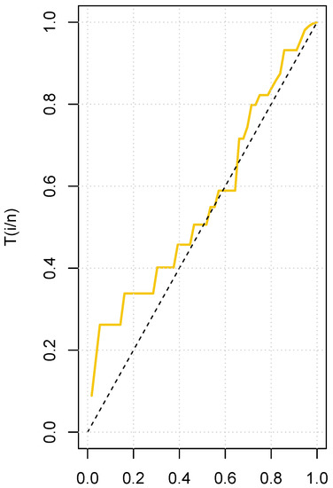
Figure 5. TTT plot for the student enrollment dataset.

To demonstrate the LIPD’s potential benefit, the distributions given in Table 4 were considered for comparison.

Table 4. The considered competitive distributions.

Distributions	Abbreviation	Reference
zero-truncated Poisson distribution	ZTPD	-
intervened Poisson distribution	IPD	[2]
zero-truncated generalized binomial distribution	ZTGBD	-
zero-truncated generalized negative binomial distribution	ZTGNBD	[23]
intervened generalized Poisson distribution	IGPD	[8]

We compare the competitive distributions to the recommended distribution using the statistical methods presented, specifically the negative log-likelihood (−logL), Akaike information criterion (AIC), Bayesian information criterion (BIC), and ${\chi }^2$ statistic. The corresponding MLEs and goodness-of-fit (GOF) results are shown in Table 5. According to Table 5, the LIPD’s GOF statistical values are lower than those of the other distributions under consideration. Therefore, the proposed model is the best choice for analyzing the provided intervention dataset.

Table 5. MLEs and GOF values for the student enrollment dataset.

Model	MLEs	$-log\mathbf{L}$	${\mathit{\chi }}^2$	$\mathit{df}$	AIC	BIC
ZTPD	$\lambda =10.9646$	311.4949	3924.5470	5	624.9899	627.6503
ZTGBD	$\lambda =19.7818$	192.1601	185.4118	3	390.3202	396.5015
	$\mu =0.1689$
	$\rho =4.0671$
ZTGNBD	$\lambda =19.8175$	192.1601	185.3881	3	390.3201	396.5015
	$\mu =0.1687$
	$\rho =3.0725$
IPD	$\rho =10.965$	311.4949	2998.871	4	626.99	631.1108
	$\lambda =0.0000012$
IGPD	$\lambda =3.3266$	192.06	187.4251	3	390.12	395.79
	$\mu =0.6607$
	$\rho =0.0647$
LIPD	$\lambda =0.0781$	191.5816	181.3314	3	389.1631	395.3444
	$\mu =0.6159$
	$\rho =20.0777$

In the case of the GLRT, the calculated value based on the test statistic in (19) is $2(-191.5816+311.4949)=119.9133$ (p-value $=0.00003$). As a result, at any level $>0.00003$, the null hypothesis is rejected in favor of the alternative hypothesis. Hence, we conclude that the additional parameter $\mu$ in the LIPD is significant in light of the test procedure outlined in Section 6.

9.2. COVID-19 Dataset

In 2019, a fresh coronavirus (COVID-19) was found in Wuhan, China. After identifying such a virus, it spread rapidly on a daily basis. To stop the virus from spreading further, various preventive actions (treatment interventions) were taken by health service agencies. Due to various interventions, we would be able to control the very large spread to some extent. Here, we consider a dataset of daily newly reported COVID-19 instances from Rwanda in East Africa, recorded between 11 October 2021 and 15 December 2021. Since the data were collected at the end of 2021, we may assume that several treatment interventions have already been applied, and hence, it is reasonable to assume the LIPD for the dataset. The data are as follows: 98, 46, 95, 86, 61, 80, 61, 17, 36, 32, 39, 36, 37, 29, 20, 57, 43, 42, 51, 63, 53, 17, 29, 38, 55, 34, 44, 33, 16, 31, 22, 19, 28, 35, 43, 11, 12, 16, 19, 7, 6, 11, 10, 15, 23, 22, 26, 8, 14, 5, 14, 5, 13, 19, 10, 13, 10, 15, 20, 15, 53, 39, 28, 50, 79, 50.

These data are accessible at http://covid19.who.int/data (accessed on 24 August 2022). Table 6 shows the descriptive measures of the data. The empirical InD of the data is equal to $15.3522$. As a result, our model employed to describe the current dataset is capable of dealing with overdispersion.

Table 6. Descriptive statistics for the COVID-19 dataset.

Statistic	n	min	${\mathit{Q}}_1$	Md	${\mathit{Q}}_3$	max	IQR
Values	66	5	15	28.50	43.75	98	28.75

In addition, Figure 6 shows an empirical TTT plot of the data, which reveals an increasing HRF.

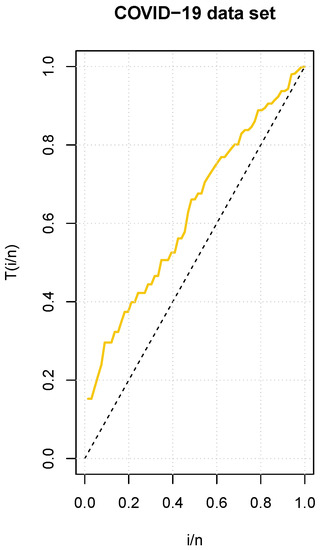
Figure 6. TTT plot for the COVID-19 dataset.

We compare the competitive distributions to the suggested distribution using the statistical techniques provided, specifically the $-\mathrm{logL}$, AIC, BIC, and ${\chi }^2$ statistic value. Table 7 displays the corresponding MLEs and GOF results, respectively. The LIPD’s MLEs and GOF statistic values are less than the other examined distributions. As a result, the suggested model is the most appropriate for modeling the given intervention dataset. Furthermore, the LIPD provides information on how effective various preventive actions taken by health service agencies were.

Table 7. MLEs and GOF values for the COVID-19 dataset.

Model	MLEs	$-log\mathbf{L}$	${\mathit{\chi }}^2$	$\mathit{df}$	AIC	BIC
ZTPD	$\lambda =32.7871$	636.744	439.98	5	1275.488	1277.677
ZTGBD	$\lambda =10.9120$	286.645	350.86	3	579.291	585.860
	$\mu =0.5095$
	$\rho =1.6295$
ZTGNBD	$\lambda =10.9112$	286.6457	350.8655	3	579.2915	585.8604
	$\mu =0.5095$
	$\rho =0.6295$
IPD	$\rho =0.1646$	636.744	439.43	4	1277.488	1281.867
	$\lambda =28.1515$
IGPD	$\lambda =2.0806$	286.5185	353.4297	3	579.037	585.606
	$\mu =0.7644$
	$\rho =2.5693$
LIPD	$\lambda =0.8959$	286.353	348.9881	3	578.7059	585.2749
	$\mu =0.7324$
	$\rho =5.0437$

In the case of the GLRT, the calculated value based on the test statistic in (19) is $2(-286.353+636.744)=350.391$ (p-value $=0.00001$). As a result, at any level $>0.00001$, the null hypothesis is rejected in favor of the alternative hypothesis. Hence, we conclude that the additional parameter $\mu$ in the LIPD is significant in light of the test procedure outlined in Section 6.

9.3. National Health Insurance Scheme

Data from the NHIS with no zero counts were collected from a health facility in Ota, Ogun State, Nigeria, for this study. A sample of 1647 patients under the NHIS was obtained from July 2016 to July 2017. There have been encounters (visits to the doctor), which is the response variable (Nencounter). If a patient was ever admitted for the period, it was indicated by the class (Eclass), which reads (in-patient = 1, out-patient = 0). The predictor (follow-up) indicates whether a patient received routine checkups or not (follow-up = 1, no follow-up = 0). The gender (sex) of the patients reads (male = 1, female = 0). Another predictor was Ndiagnosis, which represents the number of diagnoses a patient had during the period of the encounter. The last predictor included was the biological age of the patient. The data can be found on the Mendeley Elsevier website, https://data.mendeley.com/datasets/z7wznk53cf/8 accessed on 15 November 2022. Furthermore, the dataset was utilized in [29], and the authors found that, following the dispersion test, the data were underdispersed with some dispersion parameter, $\varphi =0.7806$. For $i=1,2,\dots ,1647$, the fit non-linear regression model is given by

$${\theta }_i=exp({\alpha }_0+{\alpha }_1{y}_{i1}+{\alpha }_2{y}_{i2}+{\alpha }_3{y}_{i3}+{\alpha }_4{y}_{i4}+{\alpha }_5{y}_{i5}).$$

The following regression models were used to compare the LIPRM:

• The ZTPRM given in [30].
• The ZTNBRM created in [31].
• The IPRM elaborated in [20].

Table 8 compares the performance of the LIPRM to that of the ZTPRM, ZTGPRM, and IPRM, as well as provides real-world summaries, such as the standard errors (SEs), p-values, negative log-likelihood ($-\log \mathrm{L}$), AIC, and BIC values. According to this table, the LIPRM has the lowest values across all model selection criteria, indicating that it is the best count regression model among the ZTPRM, ZTGPRM, and IPRM. Evidently, we also find that our model, which is applied to explain the current dataset, is perfectly suited to handling this underdispersion.

Table 8. The results of the regression models for the NHIS of Nigeria (SEs in brackets).

Covariates	ZTPRM		ZTNBRM		IPRM		LIPRM
	Estimate	p-Value	Estimate	p-Value	Estimate	p-Value	Estimate	p-Value
${\alpha }_0$	0.0673	<0.001	−0.1446	<0.001	1.1981	<0.001	0.1787	<0.001
	(0.0379)		(0.0541)		(0.0019)		(0.0327)
${\alpha }_1$	0.1028	<0.001	−0.0947	<0.001	0.0154	<0.001	0.0154	<0.001
	(0.0297)		(0.0409)		(0.0345)		(0.0253)
${\alpha }_2$	0.0018	<0.001	0.0045	<0.001	0.0017	<0.001	0.0017	<0.001
	(0.0007)		(0.0011)		(0.0019)		(0.0006)
${\alpha }_3$	−0.1982	<0.001	−0.07849	<0.001	−0.1406	<0.001	−0.1406	<0.001
	(0.0408)		(0.0560)		(0.0217)		(0.0329)
${\alpha }_4$	0.8705	<0.001	−1.2214	<0.001	0.1352	<0.001	0.1826	<0.001
	(0.0827)		(0.1937)		(0.0109)		(0.1046)
${\alpha }_5$	0.2919	<0.001	0.3802	<0.001	0.1352	<0.001	0.2866	<0.001
	(0.0045)		(0.0106)		(0.0109)		(0.0043)
$-\mathrm{logL}$	8379.31		3043.18		6579.37		2455.76
AIC	16,770.63		6102.36		13,172.74		4927.51
BIC	16,778.56		6112.09		13,181.25		4937.25

10. Conclusions

The LIPD, which extends the IPD and may be either underdispersed or overdispersed, was described using the Lagrangian method. There are a number of important LIPD characteristics that were identified, and it was found that they are more flexible than the IPD characteristics. We delivered specific expressions for the factorial moments: mean, variance, dispersion, skewness, kurtosis, mode, probability-generating function, moment-generating function, and cumulant-generating function. Using the classical ML method, the distribution parameters were determined. The LIPD was compared to the well-known IPD, IGPD, and some other competing distributions, and it was found that the LIPD was superior to competing models for the considered datasets. A new regression model for count data based on the LIPD was proposed and compared with its competitive regression models based on a real dataset. Three different real-world datasets—the first involving student enrollment data, the second involving COVID-19 data, and the third involving data from a health insurance scheme—were combined to show how the novel model may be applied.

References

- Cohen, A.C. Estimating parameters in a conditional Poisson distribution. Biometrics 1960, 16, 203–211. [Google Scholar] [CrossRef]
- Shanmugam, R. An intervened Poisson distribution and its medical application. Biometrics 1985, 41, 1025–1029. [Google Scholar] [CrossRef]
- Shanmugam, R. An inferential procedure for the Poisson intervention parameter. Biometrics 1992, 48, 559–565. [Google Scholar] [CrossRef]
- Huang, M.; Fung, K.Y. Intervened truncated Poisson distribution. Sankhya Ser. B 1989, 51, 302–310. [Google Scholar]
- Dhanavanthan, P. Estimation of the Parameters of Compound Intervened Poisson Distribution. Biom. J. 2000, 42, 315–320. [Google Scholar] [CrossRef]
- Kumar, C.S.; Shibu, D.S. On finite mixtures of modified intervened Poisson distribution and its applications. J. Stat. Theory Appl. 2014, 13, 344–355. [Google Scholar] [CrossRef]
- Singh, B.P.; Dixit, S.; Shukla, U. An Alternative to Intervened Poisson Distribution for Prevalence Reduction. J. Math. Stat. Sci. 2016, 2016, 730–740. [Google Scholar]
- Scollnik, D. On the Intervened Generalized Poisson Distribution. Commun. Stat.-Theory Methods 2006, 35, 953–963. [Google Scholar] [CrossRef]
- Lagrange, J.L. Mécanique Analytique; Jacques Gabay: Paris, France, 1788. [Google Scholar]
- Consul, P.C.; Shenton, L.R. Use of Lagrange expansion for generating generalized probability distributions. SIAM J. Appl. Math. 1972, 23, 239–248. [Google Scholar] [CrossRef]
- Consul, P.C.; Shenton, L.R. Some interesting properties of Lagrangian distributions. Commun. Stat. 1973, 2, 263–272. [Google Scholar] [CrossRef]
- Consul, P.C.; Famoye, F. Lagrangian Katz family of distributions. Commun. Stat. Theory Methods 1996, 25, 415–434. [Google Scholar] [CrossRef]
- Berg, K.; Nowicki, K. Statistical inference for a class of modified power series distribution with applications to random mapping theory. J. Stat. Plan. Inference 1991, 28, 247–261. [Google Scholar] [CrossRef]
- Li, S.; Black, D.; Lee, C.; Famoye, F. Dependence Models Arising from the Lagrangian Probability Distributions. Commun. Stat.-Theory Methods 2010, 29, 1729–1742. [Google Scholar] [CrossRef]
- Innocenti, A.R.; Fox, O.; Chibbaro, S. A Lagrangian probability density-function model for collisional turbulent fluid-particle flows. J. Fluid Mech. 2019, 862, 449–489. [Google Scholar] [CrossRef]
- Brito, D.; Rego, L.; Oliveira, D.; Gomes-Silva, F. Method for generating distributions and classes of probability distributions: The univariate case. Hacet. J. Math. Stat. 2019, 48, 897–930. [Google Scholar]
- Irshad, M.R.; Chesneau, C.; Shibu, D.S.; Monisha, M.; Maya, R. Lagrangian Zero Truncated Poisson Distribution: Properties Regression Model and Applications. Symmetry 2022, 14, 1775. [Google Scholar] [CrossRef]
- Irshad, M.R.; Chesneau, C.; Shibu, D.S.; Monisha, M.; Maya, R. A Novel Generalization of Zero-Truncated Binomial Distribution by Lagrangian Approach with Applications for the COVID-19 Pandemic. Stats 2022, 5, 1004–1028. [Google Scholar] [CrossRef]
- Long, J.S.; Freese, J. Regression Models for Categorical Dependent Variables Using Stata, 2nd ed.; Stata Press: College Station, TX, USA, 2005. [Google Scholar]
- Shibu, D.S. On intervened Poisson Distribution and Its Generalization. Ph.D. Thesis, University of Kerala, Thiruvananthapuram, India, 2013. submitted. [Google Scholar]
- Janardan, K.G.; Rao, B.R. Lagrangian distributions of second kind and weighted distributions. SIAM J. Appl. Math. 1983, 43, 302–313. [Google Scholar] [CrossRef]
- Janardan, K.G. A wider class of Lagrange distributions of the second kind. Commun. Stat.-Theory Methods 1997, 26, 2087–2097. [Google Scholar] [CrossRef]
- Consul, P.C.; Famoye, F. Lagrangian Probability Distributions; Birkhäuser: Boston, MA, USA, 2006. [Google Scholar]
- Rao, C.R. Minimum variance and the estimation of several parameters. Math. Proc. Camb. Philos. Soc. 1947, 43, 280–283. [Google Scholar] [CrossRef]
- Ross, S. Simulation, 5th ed.; Academic Press: Cambridge, MA, USA, 2013; pp. 5–38. [Google Scholar] [CrossRef]
- Hilbe, J.M. Negative Binomial Regression; Cambridge University Press: Cambridge, UK, 2007. [Google Scholar]
- Hardin, J.; Hilbe, J. Generalized Linear Models and Extensions, 2nd ed.; A Stata Press Publication; StatCorp LP: College Station, TX, USA, 2007. [Google Scholar]
- Aarset, M.V. How to identify a bathtub hazard rate. IEEE Trans Reliab. 1987, 36, 106–108. [Google Scholar] [CrossRef]
- Adesina, O.; Agunbiade, A.; Oguntunde, P.; Adesina, T. Bayesian Models for Zero Truncated Count Data. Asian J. Probab. Stat. 2019, 4, 1–12. [Google Scholar] [CrossRef]
- Zhao, W.; Feng, Y.; Li, Z. Zero-truncated generalized Poisson regression model and its score tests. J. East China Norm. Univ. (Nat. Sci.) 2010, 1, 17–23. [Google Scholar]
- Grogger, J.T.; Carson, R.T. Models for Truncated Counts. J. Appl. Econom. 1991, 6, 225–238. [Google Scholar] [CrossRef]
Disclaimer/Publisher’s Note: The statements, opinions and data contained in all publications are solely those of the individual author(s) and contributor(s) and not of MDPI and/or the editor(s). MDPI and/or the editor(s) disclaim responsibility for any injury to people or property resulting from any ideas, methods, instructions or products referred to in the content. |
© 2023 by the authors. Licensee MDPI, Basel, Switzerland. This article is an open access article distributed under the terms and conditions of the Creative Commons Attribution (CC BY) license (https://creativecommons.org/licenses/by/4.0/).