Article

Numerical Modeling of Erosion in Hall Effect Thrusters

CIRA, The Italian Aerospace Research Centre, Via Maiorise, 81043 Capua, Italy
*
Author to whom correspondence should be addressed.
Particles 2024, 7(1), 121-143; https://doi.org/10.3390/particles7010007
Submission received: 21 November 2023 / Revised: 22 January 2024 / Accepted: 26 January 2024 / Published: 30 January 2024
(This article belongs to the Special Issue Feature Papers for Particles 2023)

Abstract

:
The erosion of the accelerating chamber walls is one of the main factors limiting the operational life of Hall effect thrusters (HETs), and it is mainly related to the sputtering of ceramic walls due to the impacting energetic ion particles. The erosion phenomenon is investigated by means of a numerical model that couples the plasma model HYPICFLU2, used for evaluating the local distributions of ion energies and incidence angles, and a sputtering model specific for the xenon–Borosil pair, which is the most used in HETs application. The sputtering yield model is based on the measurements by Ranjan et al. that are improved with a linear factor to include wall temperature effect, recently studied by Parida et al. The experimental eroded profiles of SPT100 walls are selected as benchmark. The results show that there is a decrease in erosion speed with time, in accordance with experimental measurements, but the model underestimates, by about 50–60%, the erosion at the channel exit, which suggests a stronger dependence of sputter yield on surface temperature. Thus, the need for new experimental measurements of sputtering in the range of impact energy, angle, and wall temperature, respectively, of 10–250 eV, 0–85°, 30–600 °C, arises.

1. Introduction

Plasma propulsion uses electric power, supplied by solar panels or electric on-board generators, to accelerate ions of noble gases to high velocity (order of km/s) producing thrust. Electric propulsion devices are characterized by high specific impulse but low thrust (in the order of mN) and are most commonly used for station keeping, orbit raising maneuvers, attitude control, and orbital change from LEO to GEO [1]. They have also been recently used in interplanetary missions [2] thanks to their very long operational life (thousand of hours).
The Hall effect thruster (HET) is an electric propulsion device that generates thrust via electrostatic acceleration of ions. Thanks to its main characteristic of scalability and simplicity, HETs application for commercial satellites have been growing deeply in the last ten years (i.e., 70% of GEO and LEO satellites between 2011–2017 used HETs [1]).
The most common variant of HET, called stationary plasma thruster (SPT), ignites and sustains plasma within a discharge chamber composed of ceramic walls (the most used material is boron nitride–silica, B N - S i O 2 , named Borosil [3,4]). Thus, the term Hall thruster will be used synonymously with SPT in the rest of the paper.
HETs have cylindrical symmetry (Figure 1). A radial magnetic field, generated by coils or permanent magnets, is set at the channel exit. An external cathode provides electrons, a fraction of which move toward the anode (located at the close end of the channel), while the other part neutralizes the ions in the plume. When electrons enter the thruster (Figure 1), they become trapped in the zone of max intensity of the magnetic field, because of their small Larmor radius, so their motion to the anode is interrupted and their trajectory drifts in the azimuthal direction. In this way, a Hall current is created. The propellant, mostly noble gas (e.g., xenon, argon), is injected from the anode and is ionized by the collisions with high-energy electrons. The produced ions are accelerated by the electric field that is self-generated by the distribution of electrons along the magnetic streamlines and is perpendicular to them. For the typical magnetic field configuration (Figure 1) the axial component of the electric field accelerates part of the ions out of the channel exit, generating thrust, while the radial component pushes another one (30–40% [5]) toward the wall; these ions are, thus, accelerated into the wall by the sheath potential gradient [6]. If the energy of the impacting particle is high enough, sputtering, which is the ejection of microscopic particles from the surface of the solid material, occurs. Total removal of the ceramic results in exposure of magnetic circuitry components to plasma and effectively ends the thruster’s life [5].
Since the early 2000s, many research groups ([3,7,8,9,10,11] to name a few) have placed their efforts on the development of models to predict the erosion of the acceleration channel with the aim to accurately and rapidly assess the lifetime of thruster prototypes without the need for expensive and time-consuming life tests [3].
The bibliographic review of the published erosion models (Appendix A) has shown that:
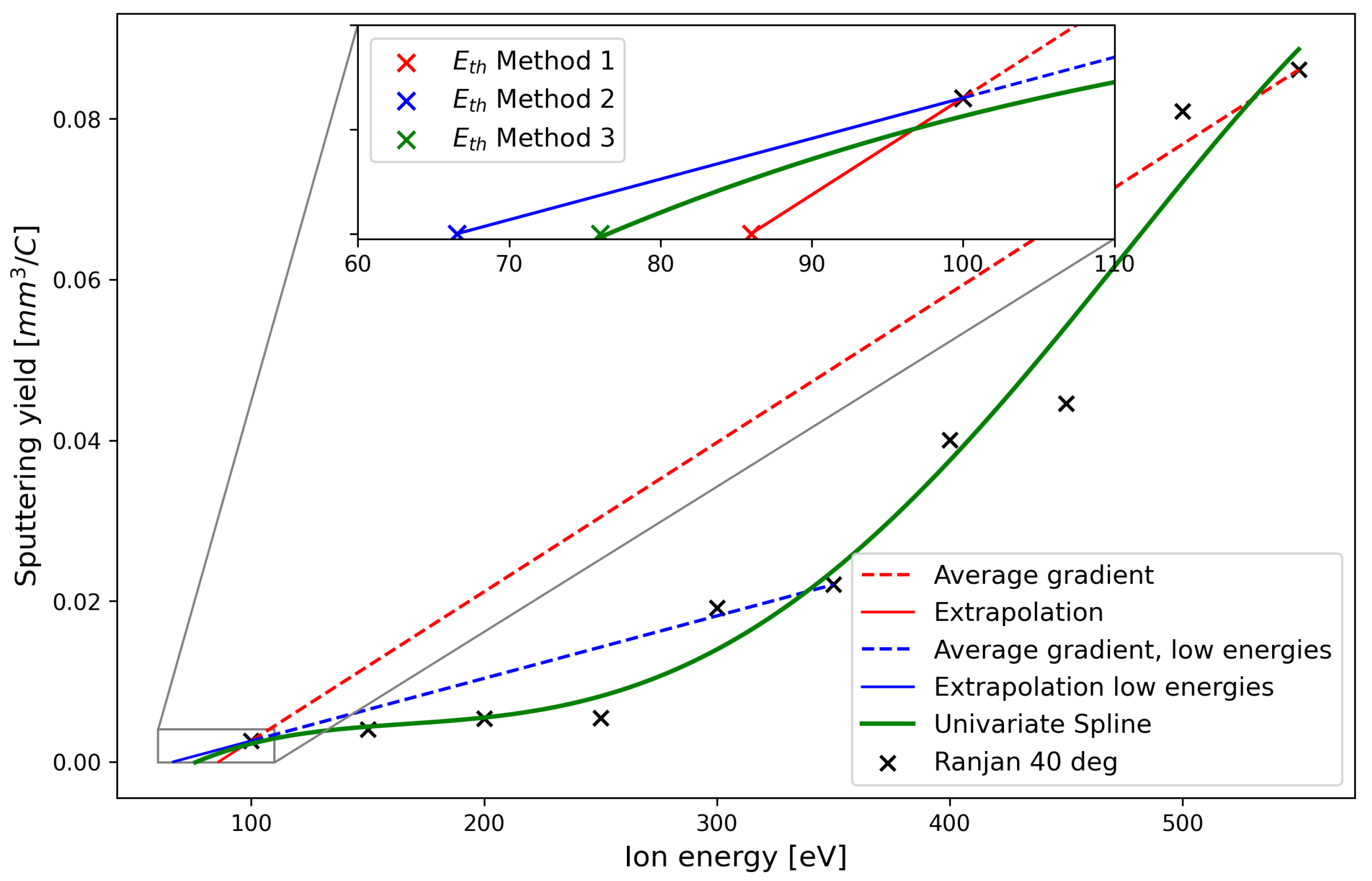
  • The threshold energy, Eth (i.e., the minimum energy of an incident particle to allow sputtering to start), is used as fitting parameter with respect to experiments;
  • The effect of wall temperature on sputtering [12] has never been taken into account;
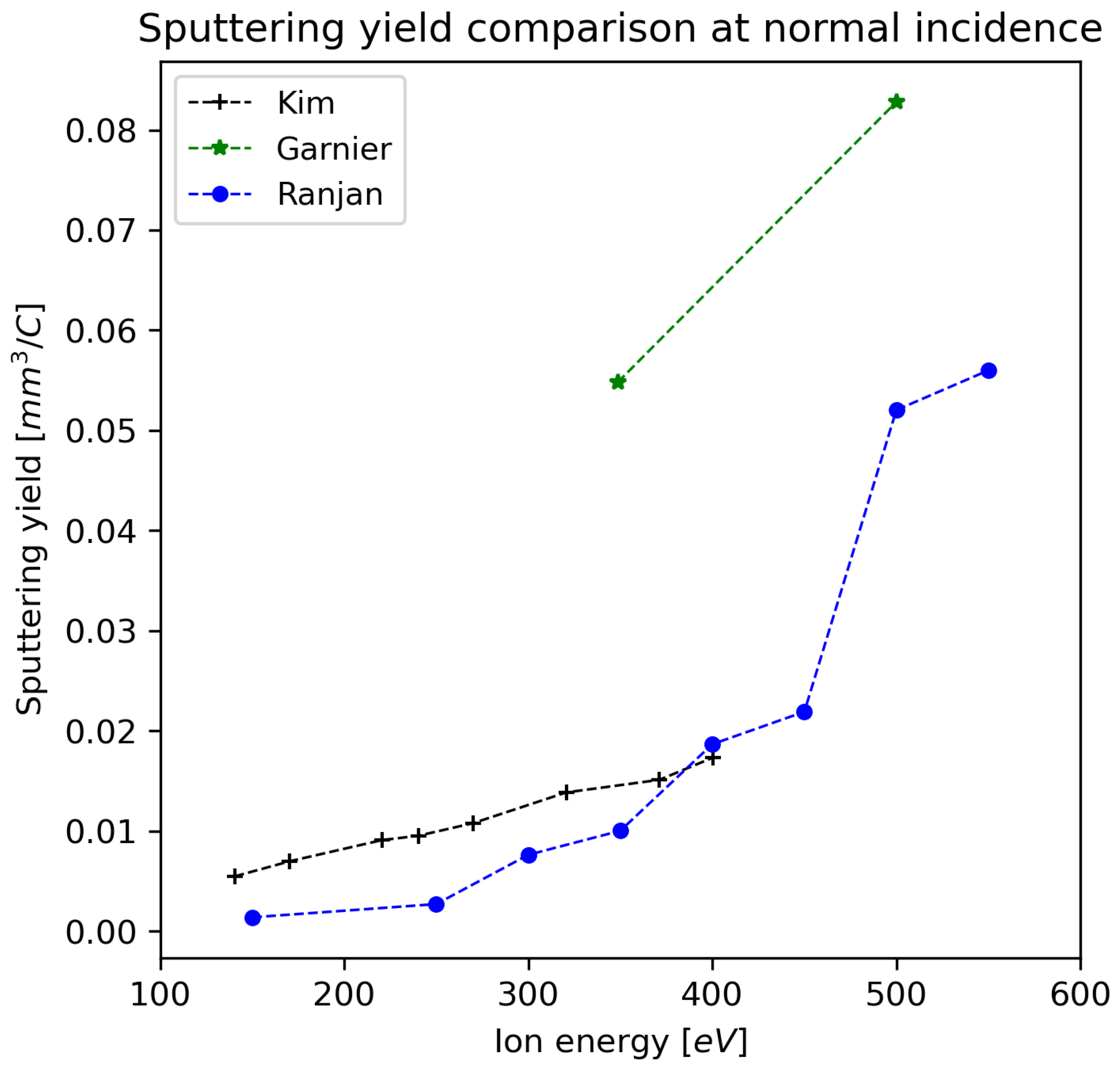
  • The most recent sputtering data regarding the Xe–Borosil couple by Ranjan et al. [13] has never been considered.
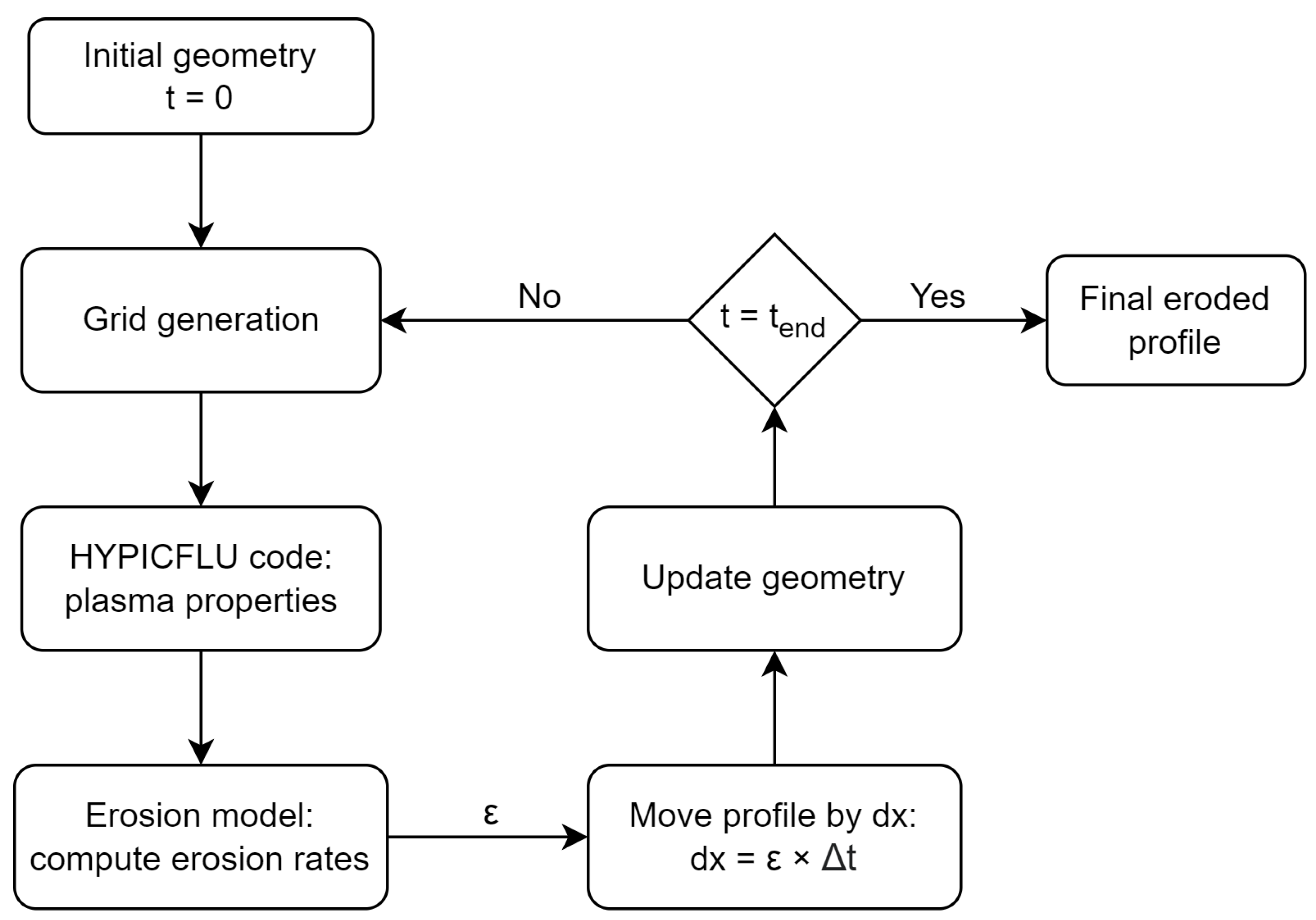
Thus, the erosion model presented in this paper aims at reducing the dependence of the sputtering on the threshold energy, by considering recent sputtering measurements ( X e B N S i O 2 ) on a wide range of incident ion energy and angles and by introducing a dependence of threshold energy on the incidence angle of impacting ions. The effect of surface temperature is considered, too. The model was used to rebuild the erosion of the SPT-100, selected as a test case because of the great availability of both experimental and numerical data in the open literature [4,14,15,16,17].
The developed erosion model is detailed in Section 2; an introduction of HYPICFLU2, the code used for the characterization of plasma within the accelerating channel, is provided in Section 2.1. The results of the erosion simulation relative to the SPT100 thruster are reported in Section 3: the erosion profiles are compared to the available experimental measurements. Finally, results are discussed and suggestions for future works are given in Section 4.

2. Erosion Model

The erosion rate, ϵ , is calculated by means of Equation (1), which is the most used approach in the open literature [3].
ϵ = Y · J i = Y ( E , θ ) · e n i v n , i E = 1 2 m i e v i 2
The sputtering yield Y (i.e., the quantity of material removed per incident ion) is multiplied with the ion current density to the wall J i (linked to the ions’ density n i and normal velocity at the wall, v n , i ) to obtain the erosion rate ϵ . In Equation (1), only singly-charged ions are considered.
The workflow to simulate erosion phenomena is schematically shown in Figure 2.
An initial computational domain (Figure 3) is generated following a given thruster geometry. The boundaries are then discretized into a finite number of nodes (Figure 4). Then, the grids required by HYPICFLU2 (Section 2.1), the code selected for the plasma simulation, are generated. From plasma calculation, the ion density and ion velocity are evaluated in order to obtain J i on the wall nodes.
Given the ion velocities at nodes, already comprising the Bohm condition, which is modeled in the plasma code, and the surface normal, it is possible to evaluate the incidence angle ( θ ). It was decided to assign the incidence angle θ i to the ith node considering the normal to the surface section included between the ith and the ith−1 nodes, as schematically shown in Figure 4. A condition has been set that, for θ π / 2 , no sputtering occurs since the flow is either parallel to the surface or divergent.
The impact energy and the incident angle are used as input in the sputtering function, which returns the volumetric sputter yield Y at a given node. Then, fixed with an operation time Δ t , the nodes are moved to allocate the new channel wall profiles. The new geometry extracted is therefore used as input in HYPICFLU2 for a new plasma simulation. The erosion simulation proceeds until the desired operation time is reached.
The following subsections detail HYPICFLU2, highlighting its most recent developments, and the sputtering model, which is the subject of this paper.

2.1. Plasma Simulation: HYPICFLU2

HYPICFLU2 (HYbrid PIC-FLUid) is a 2D axis-symmetric hybrid code developed by the Italian Aerospace Research Centre (CIRA) for the simulation of the discharge in the accelerating channel and near plume region in HETs. The particle in cell (PIC) approach [18,19] is used to calculate the ionization rate and neutrals’ and ions’ density and velocity on an elliptic mesh called the PIC grid. Electrons are treated as fluid; by solving the equations described in Ref. [19], it is possible to obtain the electron temperature, the plasma potential, and, consequently, the electric field on the nodes of a fluid grid, built from the magnetic streamlines. Data are exchanged between the two modules of the code by means of interpolation.
The first release (named HYPICFLU [19]) was characterized by a rectangular-shaped domain that included the channel and the part of the plume near the channel exit (i.e., near plume) and a simple wall sheath model similar to that of HPHall [20,21] was selected.
Because the quality of the erosion rate prediction is directly related to the evaluation of the ions’ density and normal velocity at the wall, which depends on the wall sheath model, a more detailed one was implemented. Moreover, the geometry of the domain in the plume region was transformed from a rectangle to half-circle in order to better calculate ions’ expansion, and this allows for the erosion of the corner at the channel exit.
The domain modification required the review of the numerical treatment, but the main equations are the same as described in Ref. [19]. The modifications regarding the PIC module were mainly described in Ref. [22], where the possibility to correctly simulate the plasma discharge of an HET with eroded channels was verified, too. Here, the only additional improvement regarding the wall weighting, that is the calculation of plasma density at the wall, is highlighted. For this purpose, the correct weighting (CW) method with Bohm criterion forcing (BF) was selected [23]. Thus the plasma density on the j-th boundary node is
( n e , j ) C W + B F = ( n e , j ) C W · v , W v b
where v , W is the component of ion velocity perpendicular to the wall; v b is the Bohm velocity calculated using the local electron temperature, and
( n e , j ) C W = 3 2 ( n e , j ) V W 1 2 ( n e , j + 1 ) V W
Here, pedix “VW” states a value calculated with the classic volume weighting, and j + 1 indicates the first node close to the boundary.
When dealing with the fluid module for the electrons, the method to derive the electric field from the potential was changed: the irregular-grid finite difference method (IFDM) by Xu et al. [24] was applied.
Regarding the sheath model, in HYPICFLU, according to Refs. [20,21], it was supposed that the sheath collapses after a threshold value. In HYPICFLU2, as in [25], it was considered that the sheath never collapses, and after a threshold value a new regime begins, named the charge saturation regime (CSR). As a consequence, a secondary electron flux that crosses the sheath and reaches the pre-sheath persists, thus reducing wall losses.
The secondary electron emission (SEE) yield,
δ w = Γ [ 2 + B ] A K B T e e B
was used as the threshold parameter. It is worth recalling that Γ is the Euler’s gamma function and the coefficients (A, B) depend on the wall material (e.g., for B N S i O 2 they are, respectively, 0.123 and 0.528 [4]). When δ w = δ * = 0.983 , the electric field at the wall becomes zero; this point (charge saturation limit, CSL) indicates the onset of the charged saturated regime, and is associated with a given electron temperature, T e * . For electron temperatures greater than T e * , δ w remains fixed and equal to δ * .
The sheath potential was written as a function of the SEE yield and, consequently, on electron temperature, T e , by means of Equation (5) proposed by Hofer et al. [4].
ϕ w = l n ( C 1 ( 1 δ w ) ) C 2 ( 1 δ w ) 2 C 3 ( 1 δ w ) 3 C 4 ( 1 δ w ) 4
where C 1 = 195.744 , C 2 = 1.289710 × 10 4 , C 3 = 3.454640 × 10 6 , and C 4 = 3.685070 × 10 8 for B N S i O 2 . Equation (5) is true when δ w < δ * ; when δ w > δ * :
e ϕ w T e = ϕ w * = 1.018 ϕ w = 1.018 T e e
Regarding the electron energy flux into the wall, it can be calculated by using the expression for the electron energy flux into the sheath [26], Equation (7).
q w = n e v b 2 T e 1 δ w + e ϕ w δ w < δ * q w = n e ( 1.156 v b ) 2 T e 1 δ * + e ϕ w δ w > δ *
Figure 5 shows the sheath potential and the heat flux to the wall normalized to plasma density as a function of the electron temperature by considering Borosil as the wall material.
The expected effect of implementing the CSR is clearly visible: the wall potential never becomes zero, and normalized heat flux is reduced when a secondary electron flux crosses the sheath and reaches the pre-sheath.

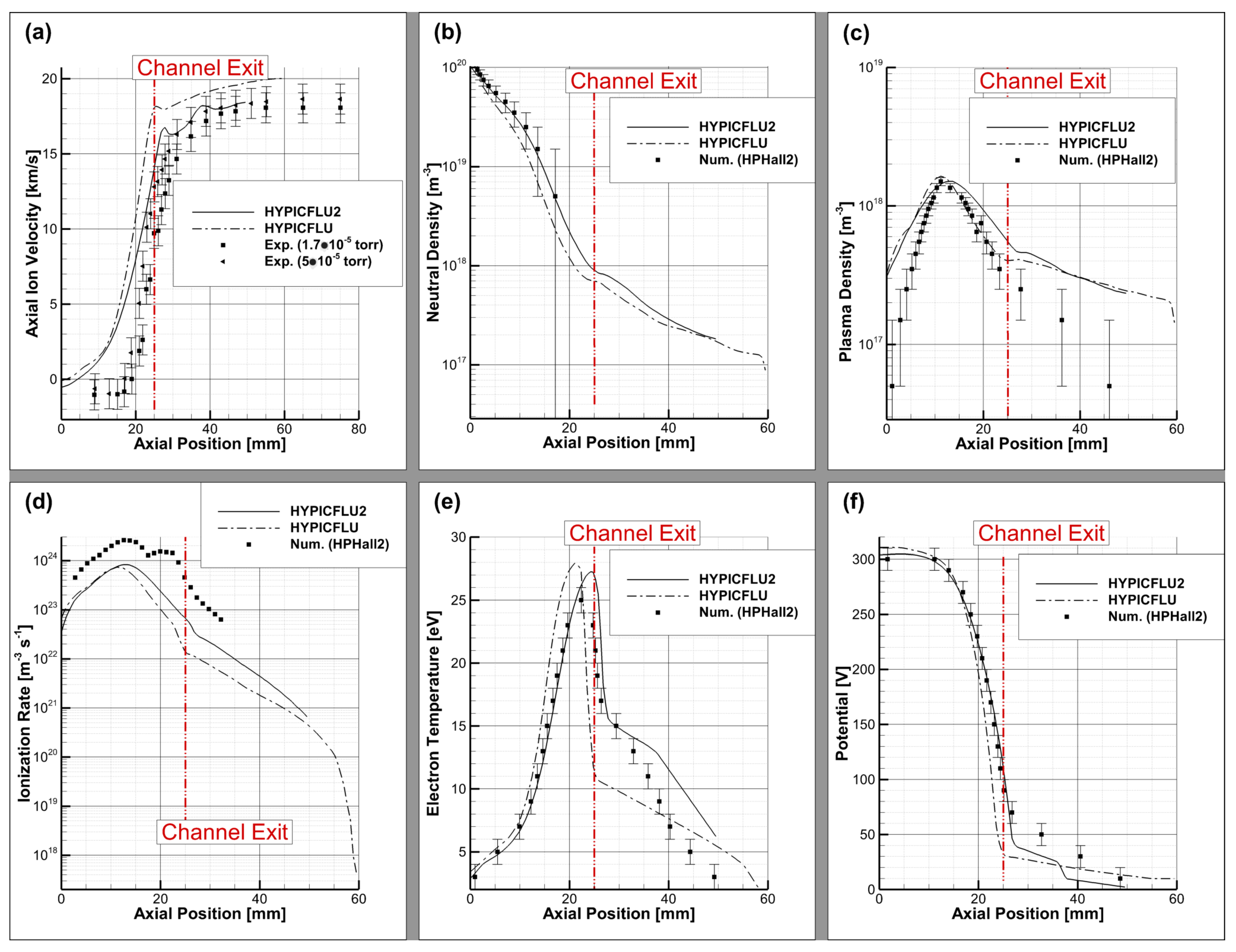
HYPICFLU2 Validation

A preliminary assessment of HYPICFLU2 was presented in Ref. [27]. Here, the main results of the last validation test are presented. These refer to the simulation of the discharge of SPT100, of which a large amount of numerical and experimental data are available in the open literature [4,14,15,16,17].
SPT100 is a 1.35 kW HET that uses coils to generate a maximum magnetic field at the exit of the thruster of about 18 mT. Its channel has a length of 25 mm, an inner radius of 35 mm, and an outer radius of 50 mm.
For the test, the same design point chosen in Ref. [19] was selected (i.e., a discharge current of 4.5 A is expected with a voltage drop of 300 V between the anode and the cathode; a xenon mass flow rate of 5 mg/s was set at the anodic inlet).
The same numerical settings and grids presented in Refs. [22,27] were used for the calculation reported here. Figure 6 reports the time-averaged plasma properties along the channel centerline (i.e., the line through the middle of the channel; radial position = 42.5 mm), namely, axial ion velocity, neutral and plasma density, ionization rate, electron temperature, and plasma potential. For the verification, the experimental measurements of the axial ion velocities by means of laser-induced fluorescence (LIF) velocimetry [17], measured at two facility background pressures (1.5 × 10⁻⁵ and 5 × 10⁻⁵ torr), were considered; furthermore, HPHall2 [4] was selected for a code–code comparison.
Axial ion velocities computed by HYPICFLU2 (Figure 6a) continuously increase along the centerline, as expected. A little counter-flow of ions, not foreseen by HYPICFLU, near the anode, is predicted. HYPICFLU2 overpredicts axial ions’ velocity with respect to the experimental data [17] in the channel, but the difference decreases moving toward the exit of it; starting from 20 mm from the anode, the data lay in the confidence bound of the experimental measurements. Neutrals perfectly match the decreasing trend detected by HPHall2 [4]. The location and the intensity of ion peaks are very well predicted. The electron temperature and potential profiles are quite in line with those selected for reference.
Thruster performances predicted by HYPICFLU2, compared to numerical and experimental data, are reported in Table 1. They were computed according to the classical formulas reported in Ref. [28]. HYPICFLU2 well predicts all the considered parameters; the slight differences must be attributed to the lower discharge current.
Figure 7 reports the normalized plasma density and the relative plasma potential to local maximum values at 18.5 mm from the anode. It is clear to see the effect of the wall sheath that decreases both density and potential, the order of magnitude of which are comparable to those reported in the literature [30,31].
Finally, it is worth underlining that HYPICFLU2 is able to reproduce HETs’ “breathing mode” oscillations [6]: the typical frequency of 22 kHz was detected by analyzing the discharge current signal.

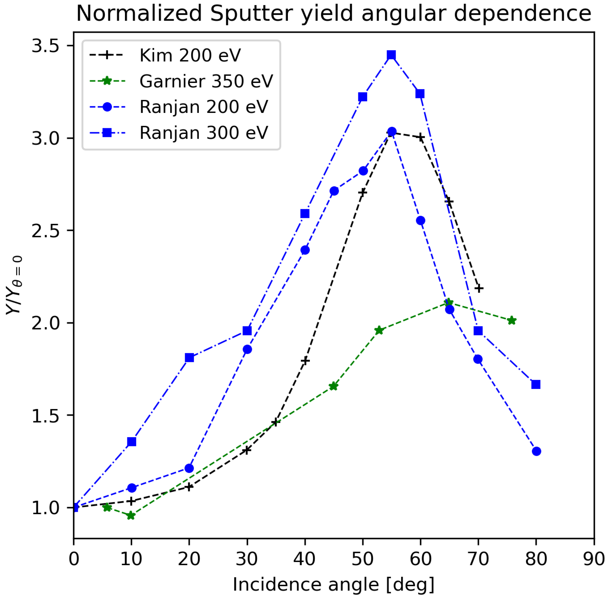
2.2. Sputtering Modeling

For the sputtering model, the recent experimental measurements of Xe ions impacting on Borosil at room temperature (300 K) by Ranjan et al. [13] were selected.
Figure 8 and Figure 9 report, respectively, the dependence of sputter yield on energy and angle, as measured by Ranjan et al. [13] compared to those collected by Garnier et al. [32], whose data were widely used to built the sputtering models available in the open literature (cfr. Appendix A). Garnier et al.’s measurements (1999) lack data for sputter yield in the energy range of interest to HETs (0–200 eV) and overestimate the sputtering yield considerably at 350 and 500 eV, whereas Ranjan’s measurements analyze the widest range of energy and angles (Figure 8 and Figure 9) and predict lower sputtering yield. Data by Kim et al.’s [33] experiments (2001) were reported for completeness, too. These are quite in line with respect to those of Ranjan, but it is worth noting that, as far as the authors know, they have never been used in sputtering modeling.
Because the study of Ranjan et al. [13] lacks data for energies lower than 100 eV (of interest to HETs application) and angles higher than 90°, extrapolations were required.
With regard to the sputter yield at incidence parallel to the surface, which is an incidence angle of 90° with respect to the surface normal, a trivial extrapolation was performed, as the sputter yield would be negligible. For that reason, the sputter yield was set equal to 0 for all the energies considered by Ranjan et al. [13] (from 100 to 550 eV in 50 eV steps), and the obtained points were added to the data collected by Ranjan et al. [13]. These points will later be included in the interpolation process, together with Ranjan’s data and the zero sputter yield energy.
Regarding the extrapolation of data below the lowest energy available, the conclusion was not as easy to reach. In particular, there is no clear value for Eth, and it may change due to composition of the material and grain orientation. Given the strong dependence of sputter yield on the angle of incidence, it was assumed that the threshold energy might as well be dependent on the incident angle of the impacting particle. This led to not fitting a single value, valid for all angles, as Eth, but instead extrapolated the available sputter yield data below 100 eV energies. Since the data considered is angular-dependent, the threshold energy will be as well.
Three simple methods were considered for the extrapolation:
  • Method 1: A linear extrapolation from the lowest energy considered by Ranjan et al. [13] (which is 100 eV) considering the average gradient between Ranjan et al.’s [13] sputter yield values, given an angle (i.e., 40 degrees, as shown in Figure 10), for all energies (from 100 to 550 eV).
  • Method 2: A linear extrapolation from the lowest energy considered by Ranjan et al. [13] (which is 100 eV) considering the average gradient between Ranjan et al.’s [13] sputter yield values, given an angle, for lower energies, in the operative range of H E T s , from 100 to 350 eV.
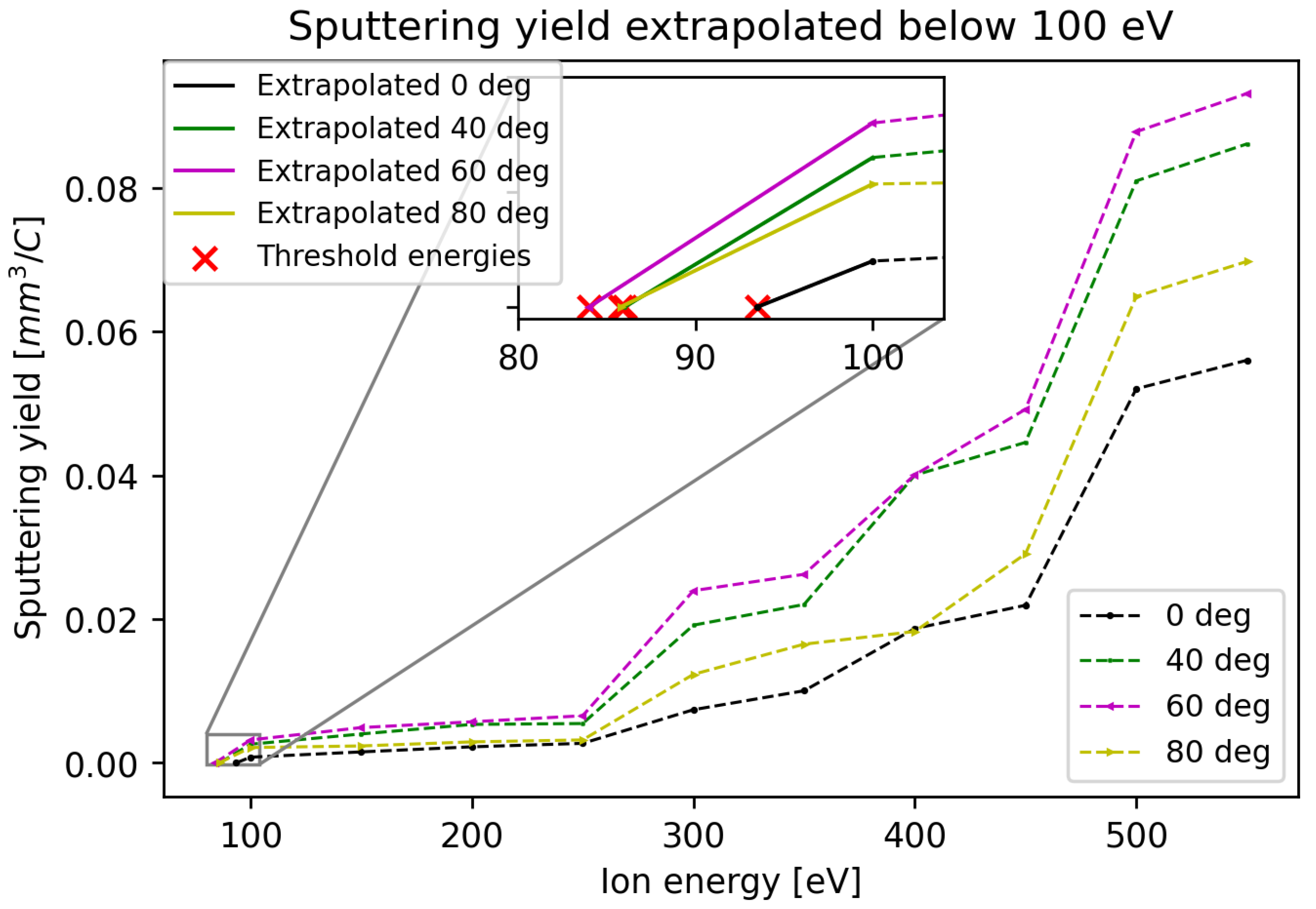
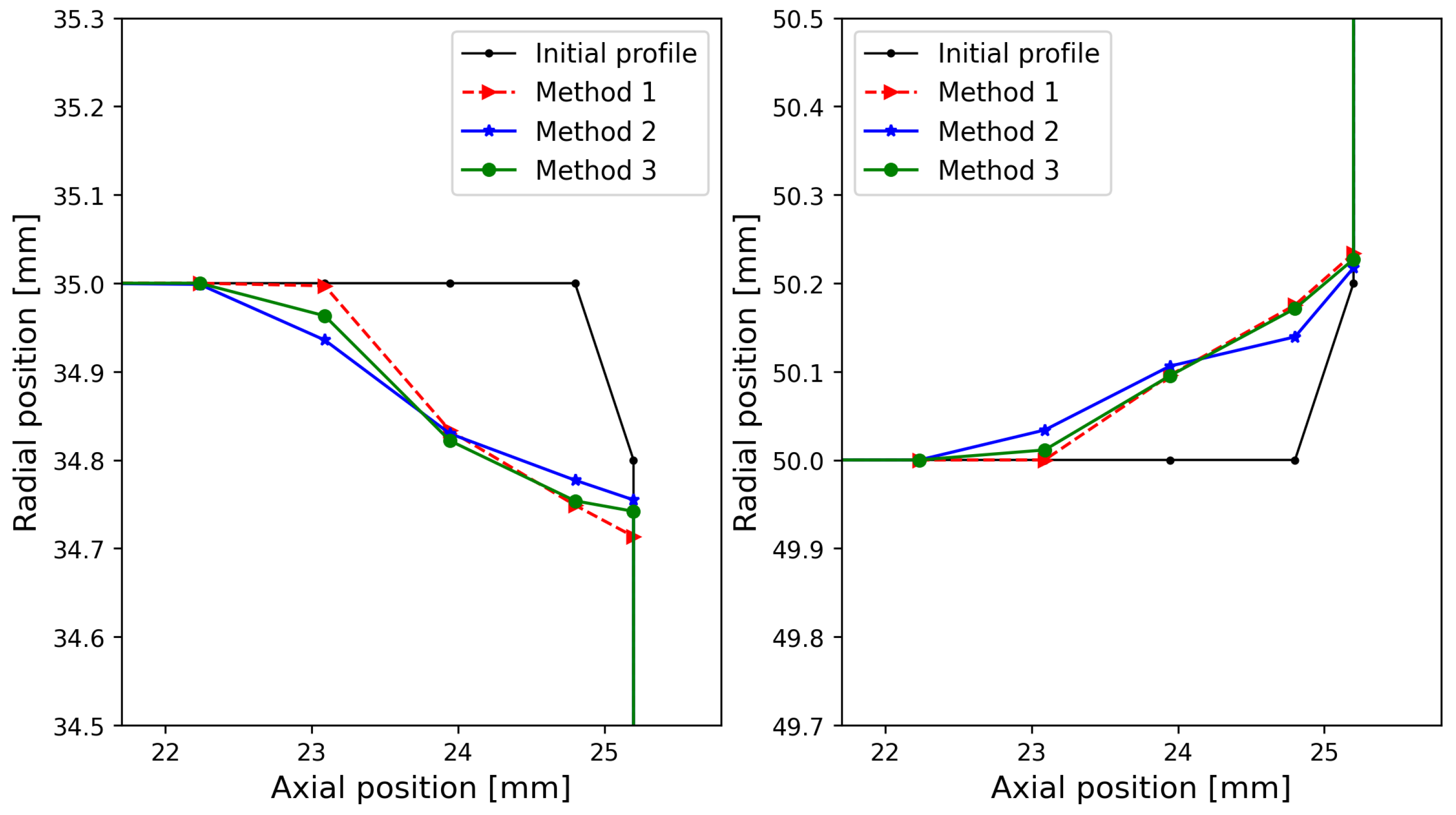
  • Method 3: An interpolation using UnivariateSpline, a built-in function in Python, which interpolates data by Ranjan et al. [13] for a given angle (all the energies) and then extrapolates to the point of interest, in particular the energy at which the sputter yield nullifies. In our case, a spline of the fourth degree was considered.
The three methods differ mainly in the value of the threshold energy extrapolated, with the linear extrapolation considering the gradient at low energies (Method 2) being the lowest and the linear extrapolation via the gradient considering all the data available (Method 1) being the highest, as can be seen in Figure 10—the threshold energy being the point at which the extrapolated line crosses the zero sputter yield line, represented with crosses in the zoom window.
As mentioned above, the threshold energy is assumed to vary with the angle of incidence since the value of the sputter yield is different for different angles. Shown in Figure 11 is the effect of angle on sputter yield and threshold energy. For compactness, only the extrapolation via the linear method (Method 1) is shown, for four different angles.
In order to join all the available data, i.e., those of Ranjan et al. [13] and the extrapolated ones, a piecewise cubic interpolation using a Clough–Tocher scheme was used [34]. The gradients of the interpolant were chosen so that the curvature of the interpolating surface is minimized. The resulting function is a surface where every point is defined by three coordinates (Figure 12). Two inputs are needed when calling the function, the angle of incidence and the energy of the impacting particle, and the output (i.e., z coordinate) is the sputter yield.
The threshold energy value influences the point at which erosion begins, but has little impact on the magnitude of erosion, as can be seen in Figure 13, where erosion profiles up to 180 h of simulated operation are shown, using the sputter yield function built on the set of data considering the Eth derived via the three different extrapolation methods. The simulation run considering the threshold energies extrapolated with Method 2, which leads to the smallest Eth, leads to an erosion which begins further up the channel, while the erosion profile considering the threshold energies extrapolated with Method 1 erodes less into the channel.
With the purpose of including the effect of temperature, the recent work of Parida et al. [12] was studied. The authors analyzed how the sputter yield of the Xe–Borosil pair at an incidence of 55° and at an energy of 500 eV vary in the range 300–873 K. The main conclusion is that there is an almost linear variation with temperature.
Even if no information about how the effect of temperature on the sputter yield changes with angle and energy, as a first guess, a linear increment with temperature, constant with both angle and energy, was assumed. This means that each value of sputter yield measured by Ranjan et al. [13] was multiplied by a coefficient, which is named the temperature coefficient ( C T ). At higher energies, with the sputter yield being greater, the difference between the original values by Ranjan et al. (Figure 12) and the ones accounting for the temperature is, thus, more pronounced.
For the extrapolation of the data beyond the experimental ones, it is again assumed that at a 90° angle of incidence the sputtering nullifies. Below 100 eV, the average gradient that was already used before was maintained, which is the average gradient of Ranjan’s data at any given angle, for two reasons:
  • The effect of temperature at different energies is unknown, and changing the gradient would imply making assumptions on such an effect. Also, Ranjan’s data [13] at room temperature is the only widespread data on which it is possible to rely;
  • Maintaining the same gradient for the extrapolation below 100 eV implicates a reduction in the minimum energy at which sputtering first occurs as temperature increases. As temperature increases, the bond strength may decrease, allowing for atoms to be sputtered from the surface at lower energies. This is yet another assumption but, given the uncertain value assigned to it in past models, it seemed a reasonable one.
For the application of one extrapolation method to the model, Method 2 was excluded because having a small gradient would lead to negative threshold energies at relatively low temperature coefficients (of about 3). Method 3 was excluded because the extrapolation of the spline would lead to the same threshold energy for any temperature coefficient used. Hence, Method 1 was selected for the rest of the simulations.
Considering a temperature coefficient, which simulates surface temperature, is equivalent to considering a higher level of sputter yield in the extrapolation region, but also in the interpolation region—Ranjan’s data are incremented by the temperature coefficient. It also implies a reduction in the threshold energy Eth; hence, sputtering of the surface occurs for ions impacting with lower energies. The effect of such increment is shown in Figure 14. The temperature coefficient is limited, due to the approximation used, as increasing the temperature coefficient too much would lead to a negative threshold energy, as shown in Figure 14, for a C T of 6.5, considering extrapolation via Method 1. A temperature coefficient of 5.5 was chosen in order to be as close as possible to experimental erosion data. The wall surface temperature is an input. We found from the open literature ([35,36]) that HETs operate at temperatures of 600 °C or higher; hence, a temperature of around 650 °C was reasonable. Due to the lack of information regarding the value of temperature along the channel axis, the temperature is considered to be constant on the surface, and equal for both the inner and outer surface. Hence, the temperature coefficient C T used in the simulation is the same for both surfaces.
In particular, the dataset upon which the sputter yield function is built is collected using three steps:
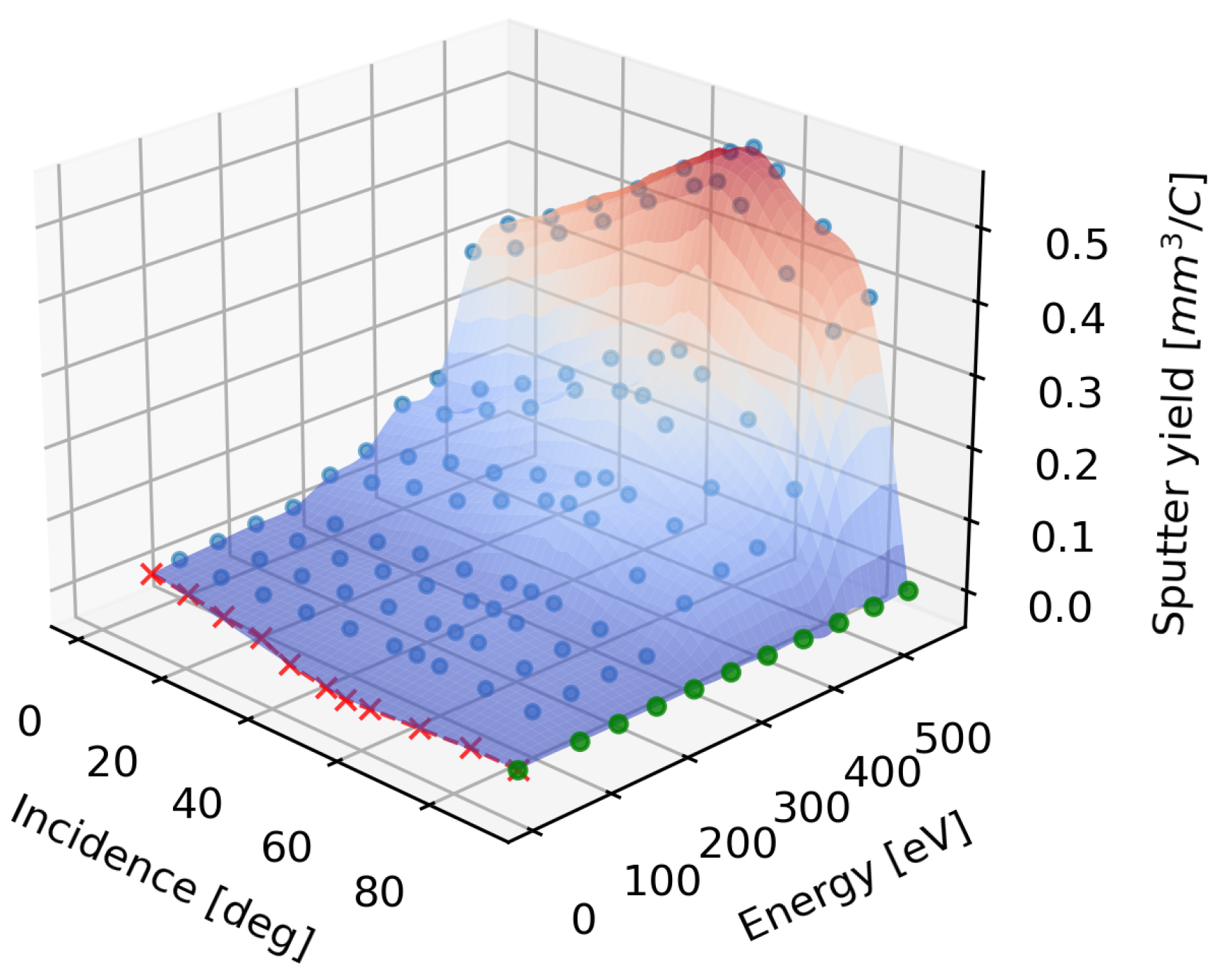
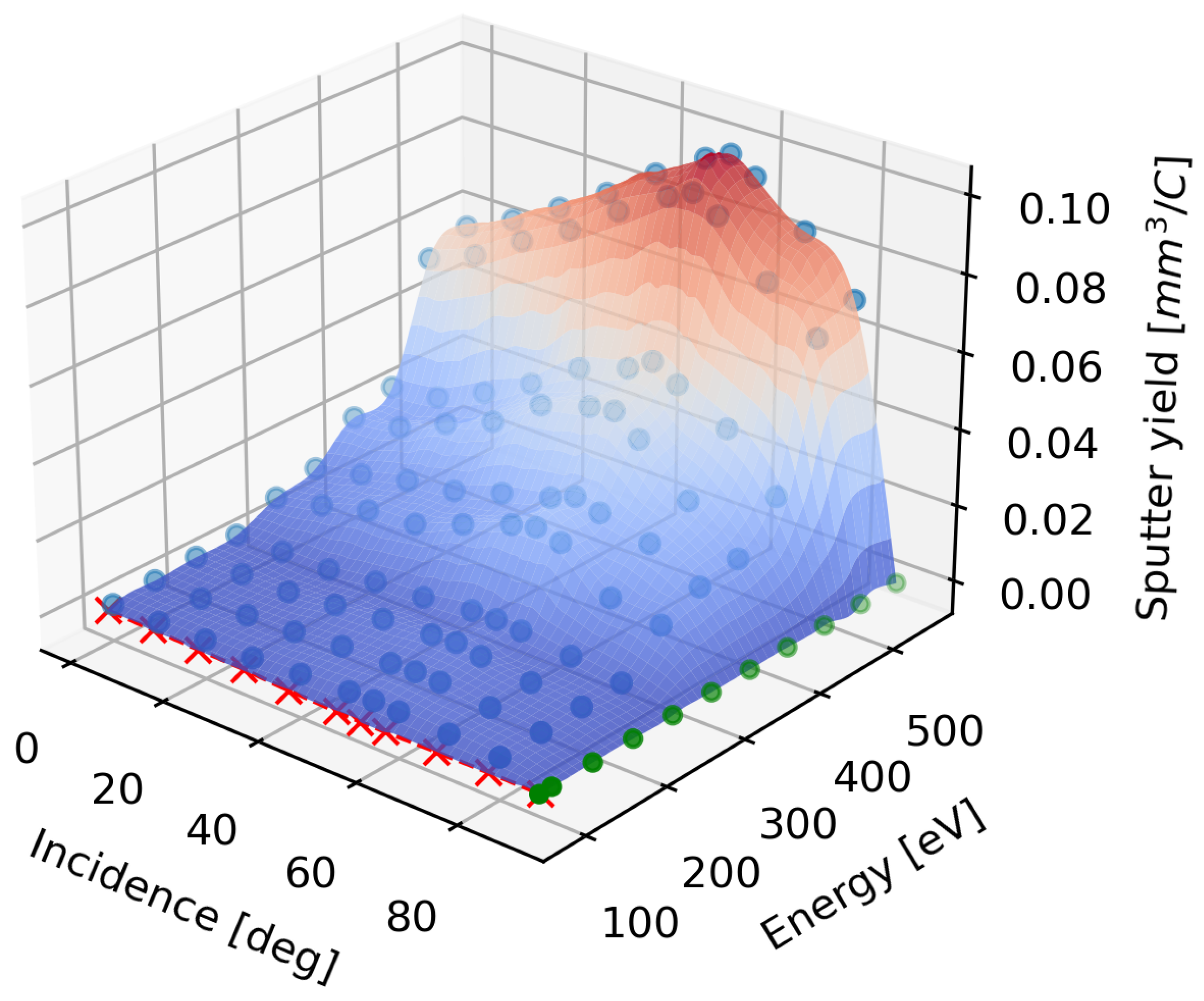
  • The set of sputter yield points at various angles and energy by Ranjan et al. [13] is multiplied by the temperature coefficient ( C T ), obtaining a new set of points with higher sputter yield values.
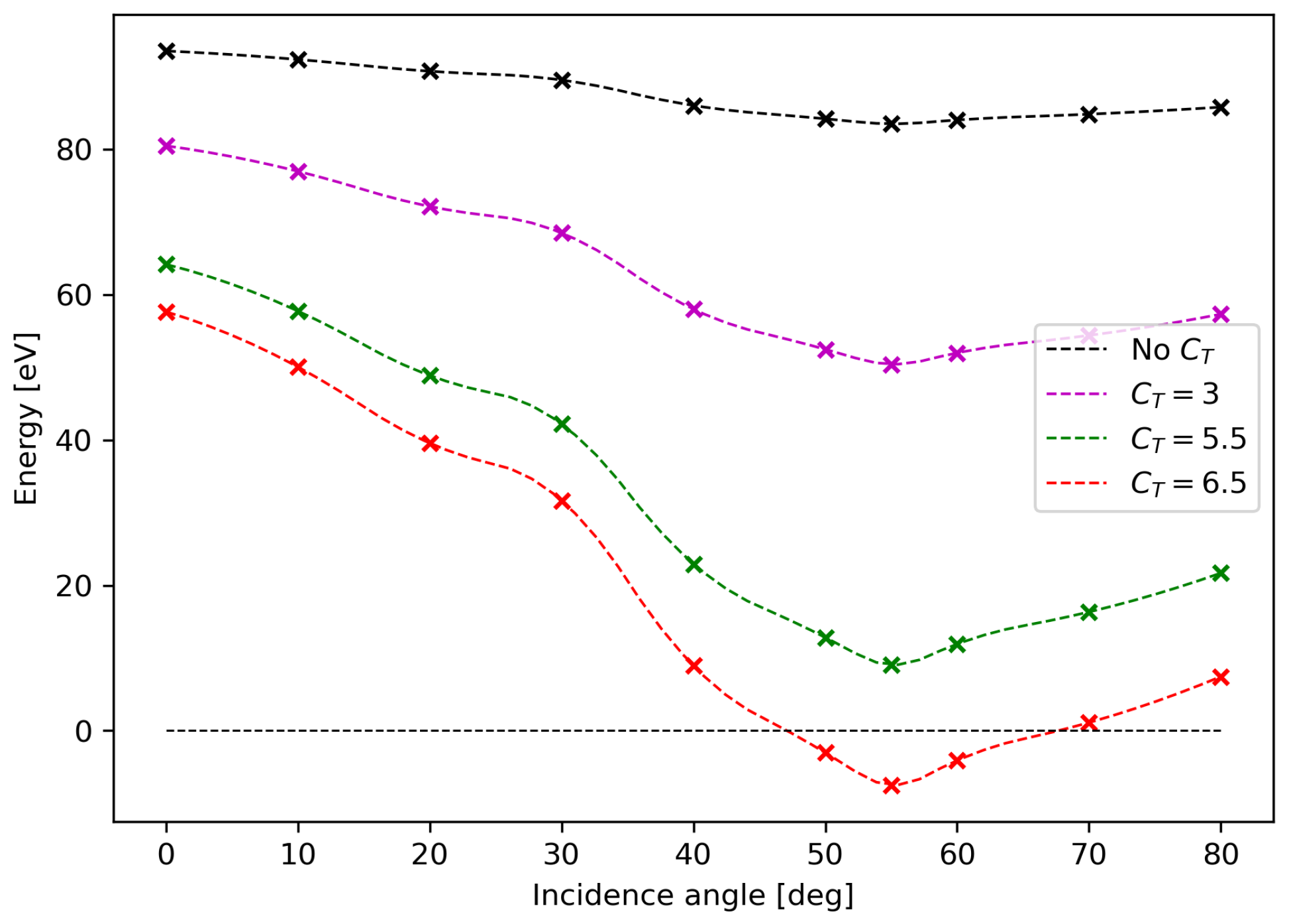
  • From the new value of sputter yield at 100 eV, incremented by C T , a value of the threshold energy for any given angle is extrapolated following the average gradient of the sputter yield value of Ranjan’s data (without the temperature coefficient—Method 1). This leads to a decrease in threshold energy for an increase in temperature coefficient; hence, simulated surface temperature.
  • Added to the set of points are the values of sputter yield at 90° of incidence angle, which is 0 for all energies.
The data considered are then joined via a piecewise cubic interpolation using a Clough–Tocher scheme, as mentioned above. The resulting surface is shown in Figure 15: the Ranjan et al. data multiplied by a temperature coefficient of 5.5 are the blue dots; the extrapolated sputter yield at 90° are the green dots, and the threshold energies extrapolated below 100 eV are the red crosses. With respect to Figure 12 the sputter yield value is higher while the threshold energy is lower.

3. Results

The erosion model described in Section 2 was used to rebuild the erosion of the SPT-100, selected as a test case because of the availability of both experimental and numerical data in the open literature [3,37].
At first, an erosion simulation using sputter yield data by Ranjan et al. [13], enlarged as described in Section 2.2 and shown in Figure 12, was run. Figure 16 shows the computed wall chamber profiles after 180 h compared to those predicted by means of Gamero et al.’s model [3] and the experimental measurements after 160 h [37]. The computed erosion is strongly underestimated if compared to experiments. The numerical predictions of Gamero et al. [3] are closer to the experimental one—nevertheless, they are based on the measurements of Garnier et al. [38] which, as seen in Section 2.2, overestimate the sputtering yield.
The gap between the experimental measurements and the numerical estimations by using “enlarged” Ranjan et al.’s [13] data was attributed to neglecting the effect of wall temperature. By introducing the temperature coefficient C T (Section 2.2), the sputter yield value, and hence the erosion, indeed increases, as demonstrated by Parida et al. [12].
Figure 17 shows the computed erosion profiles after 180 h, considering “enlarged” Ranjan et al.’s sputter yield data without the temperature coefficient (Figure 12) and with a temperature coefficient of 5.5 (Figure 15). The experimental measurements after 160 h [37] are reported for comparison. By using C T , both the erosion magnitude and length, which is the point where erosion begins with respect to the channel exit, increase.
The erosion simulation with “enlarged” Ranjan data with C T = 5.5 was further run for cumulative 1020 h in time step of 60 h (i.e., at each time step, the geometry was updated with the new profile and the plasma characteristics were simulated on the grid based on the new geometry (Section 2)). The results are shown in Figure 18 along with the experimental measurements [37]. The erosion is underestimated at each time but the point at which erosion begins is reasonably good, giving a good evaluation of activation energy Eth.
Figure 19 shows a further comparison of the computed erosion profiles and those estimated by Gamero et al. [3]. After 180 h, the curves are reasonably close; however, they differ more at increasing operational time.
Figure 20 shows the radial time evolution of the channel exit (i.e., 0.025 m away from the anode). There is a decrease in erosion speed by using “enlarged” Ranjan et al.’s data with temperature coefficient, in accordance with experimental results, as in Ref. [37]. On the contrary, Gamero et al.’s model does not show a reduction in erosion rate: wall recession is, indeed, almost linear with time. An explanation for this might be that their sputter yield model shows a small dependence of sputtering on angle at high ion incidence, which is reached when the profile deforms due to erosion.

4. Discussion

The results presented in the previous section reveal that the effect of wall temperature on sputtering yield cannot be neglected when predicting erosion in HETs’ channel, at least using the X e + –Borosil pair.
The application of the “enlarged” (Section 2.2) sputtering yield data by Ranjan et al. [13], with function only of ions impacting energy and angle, led to a strong underestimation of the erosion (Figure 16). The magnitude of the erosion at the channel exit was much smaller than the experimental one, of about 85% for the inner surface and almost 90% for the outer one. Furthermore, the predicted erosion began a lot closer to the channel exit, at around 23 mm from the anode compared to the almost 16 mm observed experimentally. This result was, most likely, due to the high zero sputter yield energy, which prevented any ion with energy below ∼83 eV from causing any erosion.
The application of a simple linear enhancement of the sputtering yield data by Ranjan et al., by means of the temperature coefficient ( C T ), led to an improvement of the prediction (i.e., the point where erosion start is correctly estimated (Figure 17)); nevertheless, the erosion was still lower than the experimental values (50% and 62% for the inner and outer surface, respectively, at the exit of the channel).
The results were obtained with C T = 5.5 , which meant considering five times the value of the sputtering yield measured at room temperature (300 K) at each energy and angle. Parida et al. [12] experimentally measured that the sputtering yield at 55° and 500 eV (which is higher than the typical value estimated in HETs’ channel, i.e., lower than 250 eV) is twice the value at room temperature.
This suggests that the effect of temperature at low energy may be more pronounced than expected. This may be because at lower energies ions penetrate less in the solid material and, hence, interact more with the surface, increasing the possibility for particles to be ejected. This may apply to incidence angle as well. This is in accordance with the Thermal Spike ( T S ) model, which is generally associated with energetic heavy particles. The basic concept of the T S model is that the small region of the surface where the highly energetic particle impacts undergoes a sudden increase in temperature, resulting in evaporation of atoms from the surface. The T S model is proposed to be the reason for the increase in sputtering observed in the experiment carried out by Parida et al. [12], too.
To obtain predictions as close as possible to experimental data, new sputtering measurements on the X e + –Borosil pair are required by considering the following ranges: impact energy 10–250 eV, angle 0–85°, and wall temperature 30–600 °C.
Moreover, further plasma code developments could help the erosion prediction. Neglecting the influence of doubly charged ions and collision between ions and neutrals, which give rise to fast moving ions, may also have an effect on it. The velocities of ions close to the surface could be underestimated, which implies a lower impacting energy and, hence, less erosion.

Author Contributions

Conceptualization, M.P. (Mario Panelli) and F.B.; methodology, M.P. (Matteo Passet) and M.P. (Mario Panelli); software, M.P. (Matteo Passet) and M.P. (Mario Panelli); validation, M.P. (Matteo Passet); formal analysis, M.P. (Matteo Passet); investigation, M.P. (Matteo Passet); data curation, M.P. (Mario Panelli) and M.P. (Matteo Passet); writing—original draft preparation, M.P. (Matteo Passet); writing—review and editing, M.P. (Mario Panelli) and F.B.; visualization, M.P. (Mario Panelli); supervision, M.P. (Mario Panelli); project administration, F.B. All authors have read and agreed to the published version of the manuscript.

Funding

This research was funded by the Italian research program in aerospace, PRORA (Programma Operativo Ricerche Aerospaziali) entrusted by MIUR (Ministero dell’Istruzione, Ministero dell’Università e della Ricerca).

Data Availability Statement

The data presented in this study are available on request from the corresponding author.

Acknowledgments

The authors would like to thank all people involved in the MEMS project and Lorenzo Casalino (Politecnico di Torino) who entrusted his graduated student to CIRA; thanks also to CIRA Space Propulsion Laboratory personnel for the stimulating research environment.

Conflicts of Interest

The authors declare no conflicts of interest.

Abbreviations

Symbols
K B Boltzmann constant
eElectron charge
m i Ion mass
ϵ Erosion rate
θ 
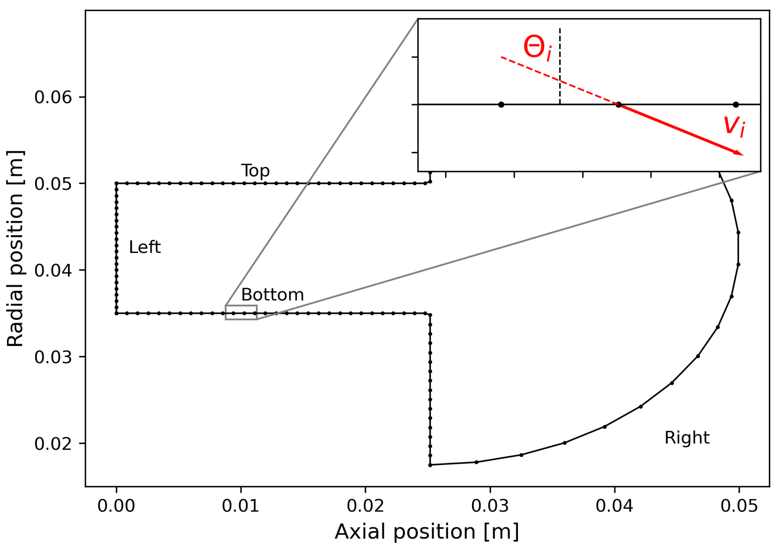
Ions incidence angle
EthThreshold energy
EIon impacting energy
vIon velocity
YSputtering yield
C t Temperature coefficient
ttime
rRadial coordinate
zAxial coordinate
nParticle number density
T e Electron temperature
ϕ Potential
ϕ * Thermalized potential
j current density vector
VVolume/voltage
Γ e Flux of electrons
δ w SEE yield
qEnergy flux to the wall
I d Discharge current
P d Discharge power
u i c Ion discharge velocity
m ˙ i c Mass flow rate
I s p Specific impulse
TThrust
η Efficiency
Subscripts
iIon
eElectron
nNeutral
wWall
e i Electron-ion
e n Electron-neutral
bBohm
Abbreviations
GEOGeostationary Earth orbit
LEOLow Earth orbit
HET(s)Hall effect thruster(s)
SPTStationary plasma thruster
PICParticle in cell
HYPICFLUHYbrid PIC-FLUid
SEESecondary electron emission
CSRCharge saturation regime
CSLCharge saturation limit
BNBoron nitride
B N S i O 2 Borosil
IFDMIrregular-grid finite difference method
CWCorrect weighting
VWVolume weighting
BFBohm criterion forcing
Xe/ X e + Xenon/ions
LIFLaser-induced fluorescence
TSThermal Spike

Appendix A. Review of Sputtering-Yield Models

A good prediction of erosion depends on a good estimation of plasma properties and sputtering. In the following, a brief overview of the sputter yield formula used in the open literature’s erosion models is presented.
Sputter yield is the quantity of material removed per incident ion or it is a measure of ejected surface material volume per time-integrated incident ion current, resulting in dimensions of volume per electric charge.
Roy and Pandey [39] proposed the following simple expression:
Y = S H s ( E i 4 H s )
Here, S = 10 2 is named as sputtering factor [38], H s = 3000 K is the sublimation energy of boron nitride (BN), and E i = 0.1 T e . The sputtering yield Y represents the number of eroded particles per incident ion at a given energy E i and at normal incidence.
Garrigues et al. [7] reported an empirical formula for the sputtering yield Y as proposed by Yamamura and Tawara [40] for the sputtering yields of metals at normal incidence. A correction factor C accounts for the effect of the angle of incidence g (defined with respect to the radial direction). This coefficient C is deduced from experimental measurements but it is not reported in the paper.
Y = Y ( E ) C ( g )
Y ( E ) = F ( E , M p , M t , Z p , Z t , β ) 1 E t h E s
Here, Z p and Z t are the atomic numbers, and M p and M t are the masses of the projectile and the target, respectively. The coefficient β and the power s are adjustable parameters, and Eth is the sputtering threshold energy. The quantities β and s are obtained by fitting for ion energies found in the SPT the analytical formula to experimental results for high Xe ion energy. Varying Eth from 30 to 70 eV leads to a same order of magnitude of Y at high ion energy but shows a strong influence on the sputtering yield at low Xe energy.
Manzella et al. [8] propose two curve fit equations for BN sputtering yield dependence on normal energy and incidence based on the data reported in Garnier et al. [32]. A threshold energy of 50 eV is assumed.
S y = f ( φ ) S ^ y φ · g ( ϵ ) S y ϵ
S ^ y φ = 1.89 · 10 7 φ 4 + 2.04 · 10 5 φ 3 3.77 · 10 4 φ 2 + 1.85 · 10 3 φ + 0.426
S y ϵ = e ( 0.0346 l n ϵ 0.136 )
Here, S y is the sputtering yield; φ is the angle with respect to normal; ϵ is, in this case, the energy of the incident ion. The sputter yield at a given wall location was found by multiplying the angle distribution, f ( φ ) , by the normalized sputter yield angular dependence by the energy distribution, g ( ϵ ) , and the sputter yield energy dependence.
Gamero and Katz [3] proposed a Yamamura and Tawara-like fit for Borosil sputtering yield dependence on energy and angle based on the Garnier et al. data [32] in the range 350 ÷ 500 eV. The energy threshold Eth is set to 58.6 eV which is a compromise between the value found in their last square estimate (56.9 eV) and the experimental value for the B N S i O 2 composite (42 ÷ 63 eV).
Y ( E , α ) = ( 0.0099 + 6.04 · 10 6 α 2 4.75 · 10 8 α 3 ) E 1 58.6 E 2.5
This formula has been proven to accurately predict erosion rates at the typical operation conditions of Hall effect thrusters, while ill-predicting erosion behavior at very low impact energies [28].
Hofer et al. [41] conducted a review of the sputtering yield data for the various grades of boron nitride under xenon bombardment. The sputtering yield is computed as a function of energy and angle from the product of two functions given by
Y ( E , θ ) = Y ( E ) Y ( θ )
where Y ( E ) is the energy-dependent yield for ions impacting the wall at normal incidence and Y ( θ ) is the angle-dependent yield relative to normal incidence. The energy-dependent yield is computed from
Y ( E ) = A E 1 E t h E 2.5
where E is the total energy of an ion impacting the wall, and the coefficients A and Eth are coefficients fit to experimental data. Here, Eth is interpreted as the threshold energy below which sputtering does not occur. The angle-dependent yield is given by
Y ( θ ) = 1 + c 0 ( 1 c o s ( c 1 θ ) ) k
where θ is the angle relative to the wall normal, and c 0 , c 1 , and k are coefficients fit to experimental data.
A few more complicated fits for the energy-dependent yield for ions impacting the wall at normal incidence were proposed by Cheng et al. [10] and used by Cho et al. [42].
Y n ( E ) = A E 0.474 1 + B E 0.3 1 E t h E 2.5
The paper reports the coefficients A and B for several energy thresholds by considering BN.
For the case of heavy-ion sputtering, the angular yield Y θ has the form
Y θ = ( Y n , E , θ i ) = Y n c o s F ( θ i ) e G
where Y n is the normal yield, E is the incident energy in electron volts, θ i is the incident angle, and F is a coefficient which depends on energy while G depends on the ion incidence angle.
In general, an adaptation of the empirical formula proposed by Yamamura et al. [40] for monoatomic solids was used for the fitting and extrapolation of sputter yield data on composites ceramics. While many formulations have been proposed and used, the most common ones are the ones proposed by Gamero et al. [3,11,43,44] and by Cheng et al. [10,45].

References

  1. Lev, D.; Myers, R.M.; Lemmer, K.M.; Kolbeck, J.; Koizumi, H.; Polzin, K. The technological and commercial expansion of electric propulsion. Acta Astronaut. 2019, 159, 213–227. [Google Scholar] [CrossRef]
  2. NASA. Ion Propulsion System. 2018. Available online: https://solarsystem.nasa.gov/missions/dawn/technology/ion-propulsion/ (accessed on 13 March 2023).
  3. Gamero-Castano, M.; Katz, I. Estimation of Hall Thruster Erosion Using HPHall. In Proceedings of the 29th International Electric Propulsion Conference, Princeton, NJ, USA, 31 October– 21 November 2005. [Google Scholar]
  4. Hofer, R.; Mikellides, I.; Katz, I.; Goebel, D. Wall Sheath and Electron Mobility Modeling in Hybrid-PIC Hall Thruster Simulations. In Proceedings of the 43rd AIAA/ASME/SAE/ASEE Joint Propulsion Conference & Exhibit, Cincinnati, OH, USA, 8–11 July 2007. [Google Scholar] [CrossRef]
  5. Ahedo, E. Plasmas for space propulsion. Plasma Phys. Control. Fusion 2011, 53, 124037. [Google Scholar] [CrossRef]
  6. Boeuf, J.P. Tutorial: Physics and modeling of Hall thrusters. J. Appl. Phys. 2017, 121, 011101. [Google Scholar] [CrossRef]
  7. Garrigues, L.; Hagelaar, G.J.M.; Bareilles, J.; Boniface, C.; Boeuf, J.P. Model study of the influence of the magnetic field configuration on the performance and lifetime of a Hall thruster. Phys. Plasmas 2003, 10, 4886–4892. [Google Scholar] [CrossRef]
  8. Manzella, D.; Yim, J.; Boyd, I. Predicting Hall Thruster Operational Lifetime. In Proceedings of the 40th AIAA/ASME/SAE/ASEE Joint Propulsion Conference and Exhibit, Fort Lauderdale, FL, USA, 11–14 July 2004. [Google Scholar] [CrossRef]
  9. Ahedo, E.; Antón, A.; Garmendia, I.; Caro, I.; del Amo, J.G. Simulation of wall erosion in Hall thrusters. In Proceedings of the International Electric Propulsion Conference, Florence, Italy, 17–20 September 2007. [Google Scholar]
  10. Cheng, S.Y.; Martinez-Sanchez, M. Hybrid Particle-in-Cell Erosion Modeling of Two Hall Thrusters. J. Propuls. Power 2008, 24, 987–998. [Google Scholar] [CrossRef]
  11. Giannetti, V.; Leporini, A.; Andreussi, T.; Andrenucci, M. Theoretical Investigation of a 5 kW Class Hall Effect Thruster. In Proceedings of the 34th International Electric Propulsion Conference, Kobe-Hyogo, Japan, 4–10 July 2015. [Google Scholar]
  12. Parida, B.K.; Sooraj, K.P.; Hans, S.; Pachchigar, V.; Augustine, S.; Remyamol, T.; Ajith, M.R.; Ranjan, M. Sputtering yield and nanopattern formation study of BNSiO2 (Borosil) at elevated temperature relevance to Hall Effect Thruster. Nucl. Instruments Methods Phys. Res. 2022, 514, 1–7. [Google Scholar] [CrossRef]
  13. Ranjan, M.; Sharma, A.; Vaid, A.; Bhatt, V.N.T.; James, M.G.; Revathi, H.; Mukherjee, S. BN/BNSiO2 sputtering yield shape profiles under stationary plasma thruster operating conditions. AIP Adv. 2016, 6, 095224. [Google Scholar] [CrossRef]
  14. Hofer, R.; Katz, I.; Mikellides, I.; Gamero-Castano, M. Heavy Particle Velocity and Electron Mobility Modeling in Hybrid-PIC Hall Thruster Simulations. In Proceedings of the 42nd AIAA/ASME/SAE/ASEE Joint Propulsion Conference & Exhibit, Sacramento, CA, USA, 9–12 July 2006. [Google Scholar] [CrossRef]
  15. Koo, J.W. Hybrid PIC-MCC Computational Modeling of Hall Thrusters. Ph.D. Thesis, The University of Michigan, Ann Arbor, MI, USA, 2005. [Google Scholar]
  16. Kawashima, R.; Komurasaki, K.; Schonherr, T.; Koizumi, H. Hybrid Modeling of a Hall Thruster Using Hyperbolic System of Electron Conservation Laws. In Proceedings of the 34th International Electric Propulsion Conference, Hyogo-Kobe, Japan, 4–10 July 2015. [Google Scholar]
  17. MacDonald-Tenenbaum, N.; Pratt, Q.; Nakles, M.; Pilgram, N.; Holmes, M.; Hargus, W. Background Pressure Effects on Ion Velocity Distributions in an SPT-100 Hall Thruster. J. Propuls. Power 2019, 35, 403–412. [Google Scholar] [CrossRef]
  18. Tskhakaya, D. The Particle-in-Cell Method. In Computational Many-Particle Physics; Fehske, H., Schneider, R., Weiße, A., Eds.; Springer: Berlin/Heidelberg, Germany, 2008; pp. 161–189. [Google Scholar] [CrossRef]
  19. Panelli, M.; Morfei, D.; Milo, B.; D’Aniello, F.A.; Battista, F. Axisymmetric Hybrid Plasma Model for Hall Effect Thrusters. Particles 2021, 4, 296–324. [Google Scholar] [CrossRef]
  20. Fife, J.M. Two-Dimensional Hybrid Particle-in-Cell Modelling of Hall Thrusters. Master’s Thesis, Massachusetts Institute of Technologies, Department of Aeronautics and Astronautics, Cambridge, MA, USA, 1995. [Google Scholar]
  21. Fife, J.M. Hybrid-PIC Modelling and Electrostatic Probe Survey of Hall Thrusters. Ph.D. Thesis, Massachusetts Institute of Technologies, Cambridge, MA, USA, 1999. [Google Scholar]
  22. Petronelli, A.; Panelli, M.; Battista, F. Particle-In-Cell Simulation of Heavy Species in Hall Effect Discharge. Aerotec. Missili Spaz. 2022, 101, 143–157. [Google Scholar] [CrossRef]
  23. Parra, F.I.; Ahedo, E.; Fife, J.M.; Martínez-Sánchez, M. A two-dimensional hybrid model of the Hall thruster discharge. J. Appl. Phys. 2006, 100, 023304. [Google Scholar] [CrossRef]
  24. Xu, G. Development of Irregular-Grid Finite Difference Method ( IFDM ) for Governing Equations in Strong Form. WSEAS Trans. Math. 2006, 5, 1117. [Google Scholar]
  25. Jolivet, L.; Roussel, J.F. Numerical modeling of plasma sheath phenomena in the presence of secondary electron emission. IEEE Trans. Plasma Sci. 2002, 30, 318–326. [Google Scholar] [CrossRef]
  26. Parra, F.I.; Ahedo, E.; Martinez-Sanchex, M.; Fife, M. Improvement of the Plasma-Wall Model on a Fluid-PIC Code of a Hall Thruster. In Proceedings of the 4th International Spacecraft Propulsion Conference, Sardinia, Italy, 2–4 June 2004; Wilson, A., Ed.; ESA Special Publication; ESA: Paris, France, 2004; Volume 555, p. 104.1. [Google Scholar]
  27. Lopedote, E.; Panelli, M.; Battista, F. Scaling of Magnetic Circuit for Magnetically Shielded Hall Effect Thrusters. Aerotec. Missili Spaz. 2023, 102, 109–125. [Google Scholar] [CrossRef]
  28. Goebel, D.; Katz, I. Fundamentals of Electric Propulsion Ion and Hall Thrusters; JPL Space Science and Technology Series; California Institute of Technology: Pasadena, CA, USA, 2008. [Google Scholar]
  29. Kwon, K. A Novel Numerical Analysis of Hall Effect Thruster and Its Application in Simultaneous Design of Thruster and Optimal Low-Thrust Trajectory. Ph.D. Thesis, Georgia Institute of Technology, Atlanta, GA, USA, 2010. [Google Scholar]
  30. Ahedo, E.; Santos, R.; Parra, F.I. Fulfillment of the kinetic Bohm criterion in a quasineutral particle-in-cell model. Phys. Plasmas 2010, 17, 073507. [Google Scholar] [CrossRef]
  31. Escobar, D.; Ahedo, E.; Parra, F.I. On conditions at the sheath boundaries of a quasineutral code for Hall thrusters. In Proceedings of the 29 th International Electric Propulsion Conference, Princeton, NJ, USA, 31 October–21 November 2005. [Google Scholar]
  32. Garnier, Y.; Viel, V.; Roussel, J.F.; Bernard, J. Low-energy xenon ion sputtering of ceramics investigated for stationary plasma thrusters. J. Vac. Sci. Technol. A 1999, 17, 3246–3254. [Google Scholar] [CrossRef]
  33. Kim, V.; Kozlov, V.; Semenov, A.; Shkarban, I. Investigation of the Boron Nitride based Ceramics Sputtering Yield Under it’s Bombardment by Xe and Kr ions. In Proceedings of the 27th International Electric Propulsion Conference, Pasadena, CA, USA, 15–19 October 2001; Available online: https://api.semanticscholar.org/CorpusID:115151109 (accessed on 25 January 2024).
  34. Alfeld, P. A bivariate C2 Clough-Tocher scheme. Comput. Aided Geom. Des. 1984, 1, 257–267. [Google Scholar] [CrossRef]
  35. Myers, J.; Kamhawi, H.; Yim, J.; Clayman, L. Hall Thruster Thermal Modeling and Test Data Correlation. In Proceedings of the American Institute of Aeronautics and Astronautics, Propulsion and Energy Conference, National Harbor, MD, USA, 25–27 July 2016. [Google Scholar]
  36. Kamhawi, H.; Liu, T.M.; Benavides, G.F.; Mackey, J.; Server-Verhey, T.; Yim, J.; Butler-Craig, N.I.; Myers, J. Performance, Stability, and Thermal Characterization of a Sub-Kilowatt Hall Thruster. In Proceedings of the 36th International Electric Propulsion Conference, Vienna, Austria, 15–20 September 2019. [Google Scholar]
  37. Absalamov, S.K.; Andreev, V.B.; Colbert, T.S.; Day, M.; Egorov, V.V.; Gnizdor, U.R.; Kaufman, H.; Kim, V.; Korakin, I.A.; Kozubsky, K.; et al. Measurement of Plasma Parameters in the Stationary Plasma Thruster (SPT-100) Plume and its Effect on Spacecraft Components. In Proceedings of the 28th Joint Propulsion Conference and Exhibit, Nashville, TN, USA, 6–8 July 1992. [Google Scholar] [CrossRef]
  38. Garnier, Y.; Viel, V.; Roussel, J.F.; Pagnon, D.; Magne, L.; Touzeau, M. Investigation of Xenon ion sputtering of one ceramic material used in SPT discharge chamber. In Proceedings of the 26th International Electric Propulsion Conference, Kitakyushu, Japan, 17–21 October 1999. [Google Scholar]
  39. Roy, S.; Pandey, B.P. Plasma–wall interaction inside a Hall thruster. J. Plasma Phys. 2002, 68, 305–319. [Google Scholar] [CrossRef]
  40. Yamamura, Y.; Tawara, H. Energy Dependence of Ion-Induced Sputtering Yields from Monoatomic Solids at Normal Incidence; Technical Report NIFS-DATA-23; National Institute for Fusion Science: Heliotron, Japan, 1995. [Google Scholar] [CrossRef]
  41. Hofer, R.R.; Mikellides, I.G.; Katz, I.; Goebel, D.M. BPT-4000 Hall Thruster Discharge Chamber Erosion Model Comparison with Qualification Life Test Data. In Proceedings of the 30th International Electric Propulsion Conference, Florence, Italy, 17–20 September 2007; Available online: https://api.semanticscholar.org/CorpusID:113891855 (accessed on 25 January 2024).
  42. Cho, S.; Yokota, S.; Kaneko, R.; Komurasaki, K.; Arakawa, Y. Channel Wall Erosion Modeling of a SPT-Type Hall Thruster. Trans. Jpn. Soc. Aeronaut. Space Sci. Aerosp. Technol. Jpn. 2012, 10, Pb25–Pb30. [Google Scholar] [CrossRef] [PubMed]
  43. Vrebosch, T.M.F.; Misuri, T.; Andrenucci, M.; Zandbergen, B.T.C. Model for Predicting the Lifetime of a Hall Effect Thruster. In Proceedings of the Space propulsion 2012 Conference, Bordeaux, France, 7–10 May 2012. [Google Scholar]
  44. Schinder, A.M.; Walker, M.L.; Rimoli, J. 3D Model for Atomic Sputtering of Heterogeneous Ceramic Compounds. In Proceedings of the 49th AIAA/ASME/SAE/ASEE Joint Propulsion Conference, San Jose, CA, USA, 14–17 July 2013. [Google Scholar] [CrossRef]
  45. Perez-Grande, D.; Fajardo, P.; Ahedo, E. Evaluation of Erosion Reduction Mechanisms in Hall Effect Thrusters. In Proceedings of the Joint Conference of 30th ISTS, 34th IEPC and 6th NSAT, Kobe-Hyogo, Japan, 4–10 July 2015. [Google Scholar]
Figure 1. Schematic illustration of a Hall thruster’s principle of functioning and sputtering phenomenon. The electric field vectors ( E ) are shown in blue, perpendicular to the magnetic field lines (B), which are shown in green. Shown in red is the plasma potential near the walls, influenced by the sheath.
Particles 07 00007 g001
Figure 2. Flow diagram for an erosion simulation.
Particles 07 00007 g002
Figure 3. Computational domain: it is composed of the channel and near plume region, which is a half-circle.
Particles 07 00007 g003
Figure 4. Definition of boundary nodes and incidence angle with respect to the surface normal (black dashed line).
Particles 07 00007 g004
Figure 5. Wall sheath potential, ϕ w , and normalized heat flux into the wall, q w . Comparison between models with (w) and without (wo) the charge saturation regime (CSR).
Particles 07 00007 g005
Figure 6. SPT-100 simulation: (a) axial ion velocity, (b) neutral and (c) plasma density, (d) ionization rate, (e) electron temperature, and (f) plasma potential as function of axial position (along a line through the middle of the channel). Data calculated by means of HYPICFLU and HYPICFLU2; experimental (Exp.) data were taken from MacDonald-Tenenbaum et al. [17] and refer to two background pressure levels within the test chamber; numerical (Num.) results were taken from Hofer et al., who used HPHall2 code [4].
Particles 07 00007 g006
Figure 7. Time-averaged radial profile of the normalized plasma density and the relative plasma potential to local maximum value, at 18.5 mm from anode; n m a x is the maximum density.
Particles 07 00007 g007
Figure 8. Normal sputter yield as function of impacting ion energies for X e + against Borosil for [13,32,33].
Particles 07 00007 g008
Figure 9. Normalized angular sputter yield as fucntion of incidence angle. X e + against Borosil [13,32,33].
Particles 07 00007 g009
Figure 10. Extrapolation of Ranjan et al.’s [13] data via three different methods. Shown in red is the linear extrapolation via Method 1, in blue is the linear extrapolation via Method 2, and in green is the extrapolation via a 4th-grade spline. The red, blue, and green crosses in the zoom window represent, respectively, the threshold energies obtained via Method 1, Method 2, and Method 3.
Particles 07 00007 g010
Figure 11. Linear extrapolation of Ranjan’s sputter yield below 100 eV, for angles of incidence of 0°, 40°, 60°, and 80°. The red crosses in the zoom window represent the zero sputter energy, hence the threshold energy for a given angle of incidence, extracted from the extrapolation (solid line).
Particles 07 00007 g011
Figure 12. Surface interpolating Ranjan et al.’s data [13] (blue dots) and the extrapolated ones—green dots are the sputter yield at 90°, red crosses are the sputter yield below 100 eV, considering the extrapolation via Method 1.
Particles 07 00007 g012
Figure 13. Eroded profiles after 180 h of simulated operation using data collection with threshold energies derived with the three different extrapolation methods.
Particles 07 00007 g013
Figure 14. Effect of temperature coefficient ( C T ) on threshold energy for impacting energy considered in the experiment by Ranjan et al. [13], extrapolated via Method 1. The crosses represent the point of zero sputter yield, for a given angle.
Particles 07 00007 g014
Figure 15. Surface interpolation of Ranjan et al.’s data [13] multiplied by a temperature coefficient of 5.5 (blue dots) and the extrapolated ones–green dots are the sputter yield at 90°, and red crosses are the sputter yield below 100 eV.
Particles 07 00007 g015
Figure 16. Comparison between computed erosion profile using “enlarged” Ranjan et al.’s data, without the effect of temperature, Gamero et al.’s profiles [3], and the experimental one [37]. (Left) inner wall; (Right) outer wall.
Particles 07 00007 g016
Figure 17. Comparison between computed erosion profile using “enlarged” Ranjan et al.’s data, with and without the effect of temperature and the experimental one [37]. (Left) inner wall; (Right) outer wall.
Particles 07 00007 g017
Figure 18. Computed and experimental [37] eroded profiles for the inner and outer surfaces of the acceleration channel.
Particles 07 00007 g018
Figure 19. Computed and Gamero et al.’s [3] eroded profiles for the inner and outer surfaces of the acceleration channel.
Particles 07 00007 g019
Figure 20. Comparison between computed, Gamero et al.’s [3], and experimental [37] wall recession at channel exit.
Particles 07 00007 g020
Table 1. SPT-100 performance: HYPICFLU2 and HYPICFLU [19] calculation vs. Exp. [29] and Num. [4] data.
Exp.Num.HYPICFLU2HYPICFLU
I d (A)4.54.54.124.65
P d (W)1350135012511395
u i c (km/s)15.717.016.219.8
m ˙ i c (mg/s)5.295.004.74.19
I s p (s)1600173316522016
T (mN)83857683
η (%)50555059
Disclaimer/Publisher’s Note: The statements, opinions and data contained in all publications are solely those of the individual author(s) and contributor(s) and not of MDPI and/or the editor(s). MDPI and/or the editor(s) disclaim responsibility for any injury to people or property resulting from any ideas, methods, instructions or products referred to in the content.

