A New Look at b → s Observables in 331 Models

Abstract

Flavour changing neutral current (FCNC) processes are described by loop diagrams in the Standard Model (SM), while in 331 models, based on the gauge group $\mathrm{SU}{\left(3\right)}_C\times \mathrm{SU}{\left(3\right)}_L\times \mathrm{U}{\left(1\right)}_X$, they are dominated by tree-level exchanges of a new heavy neutral gauge boson $Z^{\prime }$. By exploiting this feature, observables related to FCNC decays of K, $B_d$ and $B_s$ mesons can be considered in several variants of 331 models. The variants are distinguished by the value of a parameter $\beta$ that plays a key role in this framework. Imposing constraints on the $\Delta F=2$ observables, we select possible ranges for the mass of the $Z^{\prime }$ boson in correspondence to the values $\beta =\pm k/\sqrt{3}$, with $k=1,2$. The results are used to determine the impact of 331 models on $b\to s$ processes and on the correlations among them, in the light of new experimental data recently released.

1. Introduction

Flavour changing neutral current (FCNC) processes occur in the Standard Model (SM) through loop diagrams, hence they are sensitive to the virtual contribution of heavy particles, even those not yet observed. For this reason they have played a major role in the search for physics beyond the Standard Model (BSM). Among such processes, modes induced by the $b\to s$ transition have been widely investigated in theory and by the experimental collaborations. Exclusive $B\to K^{(\ast )}{\ell }^{+}{\ell }^{-}$, with $\ell =e,\mu$, offer the possibility to exploit a number of observables, such as angular distributions and asymmetries, that are sensitive to BSM. Ratios of observables are also useful, since the dependence on the Cabibbo-Kobayashi-Maskawa (CKM) matrix elements drops out. The largest uncertainty is related to the hadronic form factors describing the $B\to K^{(\ast )}$ matrix elements. Some observables can be identified where such an uncertainty is largely reduced. Other interesting modes in this category are $B_s\to {\mu }^{+}{\mu }^{-}$ and $B\to K^{(\ast )}\nu \overline{\nu }$. Tensions with respect to the SM predictions have emerged in experimental data relative to these modes [1].

Among the various scenarios proposed to extend the SM, promising ones are the 331 models based on the gauge group $\mathrm{SU}{\left(3\right)}_C\times \mathrm{SU}{\left(3\right)}_L\times \mathrm{U}{\left(1\right)}_X$, in which FCNC processes are dominated by tree-level exchanges of a new heavy neutral gauge boson $Z^{\prime }$. In this paper we consider how these models face the latest experimental results for a few observables relative to the modes $B\to K^{(\ast )}{\ell }^{+}{\ell }^{-}$ and $B\to K^{(\ast )}\nu \overline{\nu }$.

The plan of the paper is the following. In Section 2 we review the main features of the 331 models that are relevant for our study, specifying the classification of the model variants. A new approach to constrain the 331 parameters independently of the variant, and to bound the $Z^{\prime }$ mass in the four considered variants is provided in Section 3. The SM effective Hamiltonians for $b\to s{\ell }^{+}{\ell }^{-}$ and $b\to s\nu \overline{\nu }$ are presented in Section 4, as well as their modification in the 331 case. The results of our study are discussed in Section 5. The last section is devoted to the conclusions.

2. The 331 Models

We briefly describe the class of models that goes under the name of 331 models [2,3], focusing on the features relevant for our discussion. A detailed description can be found in [4].

The 331 models are based on the gauge group $\mathrm{SU}{\left(3\right)}_C\times \mathrm{SU}{\left(3\right)}_L\times \mathrm{U}{\left(1\right)}_X$, first spontaneously broken into the SM one $\mathrm{SU}{\left(3\right)}_C\times \mathrm{SU}{\left(2\right)}_L\times \mathrm{U}{\left(1\right)}_Y$, then to $\mathrm{SU}{\left(3\right)}_C\times \mathrm{U}{\left(1\right)}_Q$.

The important differences with respect to the SM, consequences of having enlarged the gauge group, are listed below.

• Five new gauge bosons are introduced.
• Left-handed fermions can transform according to the fundamental or the conjugate representation of $\mathrm{SU}{\left(3\right)}_L$, i.e., as triplets or antitriplets. New heavy fermions can also be present. Right-handed fermions are singlets as in SM. This model can answer the conceptual question of why the number of fermion generations is three. Indeed, requiring that gauge anomalies cancel and that asymptotic freedom occurs in QCD constrains the number of generations to be equal to the number of colours. However, this holds provided that quark generations transform differently under $\mathrm{SU}{\left(3\right)}_L$. It is usually assumed that the the first two quark generations transform as triplets, while the third generation and the leptons transform as antitriplets. Another possibility is obtained reversing the role of triplets and antitriplets.
• The Higgs sector is extended, and consists of three $\mathrm{SU}{\left(3\right)}_L$ triplets and one sextet.
• The electric charge operator $\widehat{Q}$ is defined as

  $$\begin{array}{c}\hfill \widehat{Q}={\widehat{T}}_3+\beta {\widehat{T}}_8+\widehat{X},\end{array}$$

  with ${\widehat{T}}_3$ and ${\widehat{T}}_8$ the diagonal $\mathrm{SU}{\left(3\right)}_L$ generators and $\widehat{X}$ the $\mathrm{U}{\left(1\right)}_X$ generator.

Among 331 models, a given variant is specified by a parameter $\beta$ together with the choice between the two possibilities for the fermion representations. Even though the charges of the new gauge bosons depend on the variant, one of them, usually denoted $Z^{\prime }$, is neutral regardless of the value of $\beta$. This new gauge boson mediates tree-level FCNC in the quark sector, while its couplings to leptons are diagonal and universal.

To define quark mass eigenstates, two rotation matrices are introduced as in the SM. The one that rotates up-type quarks is denoted as $U_L$, for down-type quarks it is $V_L$. The relation $V_{\mathrm{CKM}}=U_L^{†}{V}_L$ holds, $V_{\mathrm{CKM}}$ being the CKM matrix. Differently from the SM, where $V_{\mathrm{CKM}}$ weights the charged current interactions between up- and down-type quarks and where the two matrices $U_L$ and $V_L$ never appear individually, in 331 models only one between $U_L$ or $V_L$ can be expressed in terms of $V_{\mathrm{CKM}}$ and of the other one, so that the remaining rotation matrix affects the $Z^{\prime }$ couplings to quarks. Choosing $V_L$ as the remaining matrix, the following parametrization can be adopted:

$$\begin{array}{c}\hfill V_L=\left(\begin{array}{ccc}{\tilde{c}}_{12}{\tilde{c}}_{13}& {\tilde{s}}_{12}{\tilde{c}}_{23}{e}^{i{\delta }_3}-{\tilde{c}}_{12}{\tilde{s}}_{13}{\tilde{s}}_{23}{e}^{i({\delta }_1-{\delta }_2)}& {\tilde{c}}_{12}{\tilde{c}}_{23}{\tilde{s}}_{13}{e}^{i{\delta }_1}+{\tilde{s}}_{12}{\tilde{s}}_{23}{e}^{i({\delta }_2+{\delta }_3)}\\ -{\tilde{c}}_{13}{\tilde{s}}_{12}{e}^{-i{\delta }_3}& {\tilde{c}}_{12}{\tilde{c}}_{23}+{\tilde{s}}_{12}{\tilde{s}}_{13}{\tilde{s}}_{23}{e}^{i({\delta }_1-{\delta }_2-{\delta }_3)}& -{\tilde{s}}_{12}{\tilde{s}}_{13}{\tilde{c}}_{23}{e}^{i({\delta }_1-{\delta }_3)}-{\tilde{c}}_{12}{\tilde{s}}_{23}{e}^{i{\delta }_2}\\ -{\tilde{s}}_{13}{e}^{-i{\delta }_1}& -{\tilde{c}}_{13}{\tilde{s}}_{23}{e}^{-i{\delta }_2}& {\tilde{c}}_{13}{\tilde{c}}_{23}\end{array}\right),\end{array}$$

(1)

with ${\tilde{c}}_i=\cos {\theta }_i$, ${\tilde{s}}_i=\sin {\theta }_i$ and phases ${\delta }_{1,2,3}$.

It is worth noticing that flavour violating $Z^{\prime }$ couplings to quarks involve few parameters in (1) depending on the decay we are considering. Indeed, the $B_d$ system involves ${\tilde{s}}_{13}$ and ${\delta }_1$, the $B_s$ system involves ${\tilde{s}}_{23}$ and ${\delta }_2$, the kaon system ${\tilde{s}}_{13}$, ${\tilde{s}}_{23}$ and ${\delta }_2-{\delta }_1$, providing a remarkable correlation among the three systems [4,5,6,7,8,9]. Moreover, the relation

$$\begin{array}{c}\hfill U_L=V_L{V}_{\mathrm{CKM}}^{†}\end{array}$$

(2)

allows one to constrain the $Z^{\prime }$ mediated FCNC transitions of up-type quark using bounds established in down-type quark sector [10,11]. Such a connection between down-type and up-type quark FCNC processes is a peculiar feature of the 331 models. The 331 Lagrangian density describing the $Z^{\prime }$ coupling to ordinary fermions, for a generic value $\beta$, is:

$$\begin{array}{cc}\hfill i{\mathcal{L}}_{\mathrm{int}}^{Z^{\prime }}& =i\frac{g{Z}^{\prime \mu }}{2\sqrt{3}{c}_W\sqrt{1-(1+{\beta }^2)s_W^2}}\times \hfill \\ \hfill & \times \left\{\sum _{\ell =e,\mu ,\tau }\right\{\left[1-(1+\sqrt{3}\beta )s_W^2\right]\left({\overline{\nu }}_{\ell L}{\gamma }_{\mu }{\nu }_{\ell L}+{\overline{\ell }}_L{\gamma }_{\mu }{\ell }_L\right)-2\sqrt{3}\beta s_W^2{\overline{\ell }}_R{\gamma }_{\mu }{\ell }_R+\hfill \\ \hfill & +\sum _{i,j=1,2,3}\{\left[-1+\left(1+\frac{\beta }{\sqrt{3}}\right)s_W^2\right]{\left({\overline{q}}_{uL}\right)}_i{\gamma }_{\mu }{\left(q_{uL}\right)}_j{\delta }_{ij}+2c_W^2{\left({\overline{q}}_{uL}\right)}_i{\gamma }_{\mu }{\left(q_{uL}\right)}_j{u}_{3i}^{*}{u}_{3j}+\hfill \\ \hfill & +\left[-1+\left(1+\frac{\beta }{\sqrt{3}}\right)s_W^2\right]{\left({\overline{q}}_{dL}\right)}_i{\gamma }_{\mu }{\left(q_{dL}\right)}_j{\delta }_{ij}+2c_W^2{\left({\overline{q}}_{dL}\right)}_i{\gamma }_{\mu }{\left(q_{dL}\right)}_j{v}_{3i}^{*}{v}_{3j}+\hfill \\ \hfill & +\frac{4}{\sqrt{3}}\beta s_W^2{\left({\overline{q}}_{uR}\right)}_i{\gamma }_{\mu }{\left(q_{uR}\right)}_j{\delta }_{ij}-\frac{2}{\sqrt{3}}\beta s_W^2{\left({\overline{q}}_{dR}\right)}_i{\gamma }_{\mu }{\left(q_{dR}\right)}_j{\delta }_{ij}\},\hfill \end{array}$$

(3)

with $s_W=\sin {\theta }_W$ and $c_W=\cos {\theta }_W$, $q_u$ ($q_d$) denoting an up-type (down-type) quark (i, j are generation indices), and $u_{ij}$ and $v_{ij}$ are, respectively, the elements of $U_L$ and $V_L$ matrices. Following [4] we write the $Z^{\prime }$ couplings to down-type quarks as:

$$\begin{array}{c}\hfill i{\mathcal{L}}_L\left(Z^{\prime }\right)=i\left[{\Delta }_L^{sd}\left(Z^{\prime }\right)\left(\overline{s}{\gamma }^{\mu }{P}_{L}d\right)+{\Delta }_L^{bd}\left(Z^{\prime }\right)\left(\overline{b}{\gamma }^{\mu }{P}_{L}d\right)+{\Delta }_L^{bs}\left(Z^{\prime }\right)\left(\overline{b}{\gamma }^{\mu }{P}_{L}s\right)\right]Z_{\mu }^{\prime },\end{array}$$

(4)

the first upper index denotes the outgoing quark, while the second index the incoming one, so that:

$$\begin{array}{c}\hfill {\Delta }_L^{ji}\left(Z^{\prime }\right)={\left[{\Delta }_L^{ij}\left(Z^{\prime }\right)\right]}^{*}.\end{array}$$

(5)

The $Z^{\prime }$ couplings to leptons are defined analogously; they are denoted as ${\Delta }_L^{\nu \overline{\nu }}\left(Z^{\prime }\right)$ and ${\Delta }_{L,R}^{\mu \overline{\mu }}\left(Z^{\prime }\right)$. We list these couplings below, since they play a central role in our discussion:

$$\begin{array}{cc}\hfill {\Delta }_L^{sd}\left(Z^{\prime }\right)& =\frac{g{c}_W}{\sqrt{3}}\sqrt{f\left(\beta \right)}{v}_{32}^{*}{v}_{31},\hfill \end{array}$$

(6a)

$$\begin{array}{cc}\hfill {\Delta }_L^{bd}\left(Z^{\prime }\right)& =\frac{g{c}_W}{\sqrt{3}}\sqrt{f\left(\beta \right)}{v}_{33}^{*}{v}_{31},\hfill \end{array}$$

(6b)

$$\begin{array}{cc}\hfill {\Delta }_L^{bs}\left(Z^{\prime }\right)& =\frac{g{c}_W}{\sqrt{3}}\sqrt{f\left(\beta \right)}{v}_{33}^{*}{v}_{32},\hfill \end{array}$$

(6c)

$$\begin{array}{cc}\hfill {\Delta }_L^{\mu \overline{\mu }}\left(Z^{\prime }\right)& ={\Delta }_L^{\nu \overline{\nu }}\left(Z^{\prime }\right)=\frac{g\left[1-(1+\sqrt{3}\beta )s_W^2\right]}{2\sqrt{3}{c}_W\sqrt{1-(1+{\beta }^2)s_W^2}},\hfill \end{array}$$

(7a)

$$\begin{array}{cc}\hfill {\Delta }_R^{\mu \overline{\mu }}\left(Z^{\prime }\right)& =\left\{\begin{array}{c}\frac{-g\beta s_W^2}{c_W\sqrt{1-(1+{\beta }^2)s_W^2}}\mathrm{for}\beta \ne \sqrt{3}\hfill \\ \frac{g\sqrt{1-4s_W^2}}{\sqrt{3}{c}_W}\mathrm{for}\beta =\sqrt{3}\hfill \end{array}\right..\hfill \end{array}$$

(7b)

Notice that the $Z^{\prime }$ couplings to leptons are the same for all generations, so that the Lepton Flavour Universality is not violated in 331 models, as in the SM.

The $Z-Z^{\prime }$ mixing, negligible in $\Delta F=2$ transitions, involves the mixing angle is written as [6].

$$\begin{array}{c}\hfill \sin \xi =\frac{c_W^2}{3}\sqrt{f\left(\beta \right)}\left(3\beta \frac{s_W^2}{c_W^2}+\sqrt{3}a\right)\left[\frac{M_Z^2}{M_{Z^{\prime }}^2}\right]\equiv B(\beta ,a)\left[\frac{M_Z^2}{M_{Z^{\prime }}^2}\right],\end{array}$$

(8)

where

$$\begin{array}{c}\hfill f\left(\beta \right)=\frac{1}{1-(1+{\beta }^2)s_W^2}>0.\end{array}$$

(9)

The parameter a introduced in Equation (8) is defined as follows:

$$\begin{array}{c}\hfill -1<a=\frac{v_{-}^2}{v_{+}^2}<1,\end{array}$$

(10)

with $v_{\pm }$ related to the VEVs of two Higgs triplets $\rho$ and $\eta$,

$$\begin{array}{c}\hfill v_{+}^2=v_{\eta }^2+v_{\rho }^2,v_{-}^2=v_{\eta }^2-v_{\rho }^2.\end{array}$$

(11)

a can be written in terms of the parameter $\tan \overline{\beta }$ as

$$\begin{array}{c}\hfill a=\frac{1-{\tan }^2\overline{\beta }}{1+{\tan }^2\overline{\beta }},\tan \overline{\beta }=\frac{v_{\rho }}{v_{\eta }}.\end{array}$$

(12)

Finally, the $\mathrm{U}{\left(1\right)}_X$ gauge coupling $g_X$ and the $\mathrm{SU}{\left(3\right)}_L$ coupling g obey the relation

$$\begin{array}{c}\hfill \frac{g_X^2}{g^2}=\frac{6{\sin }^2{\theta }_W}{1-(1+{\beta }^2){\sin }^2{\theta }_W}.\end{array}$$

(13)

Depending on the different values of $\beta$ and $\tan \overline{\beta }$, it is possible to define 24 different 331 models, called $M_i$ with $i=\{1,2,\cdots ,24\}$. Each one of them is analyzed in two scenarios, called $F_1$ and $F_2$, where $F_1$ stands for the case having two generations of quarks belonging to triplets of $\mathrm{SU}{\left(3\right)}_L$ and the third generation to antitriplets; otherwise for $F_2$. Four out of 24 models have been selected in the present analysis, corresponding to the $F_1$ scenario and $\tan \overline{\beta }=1$. They are [9]:

$$\begin{array}{c}\hfill M_1⟷\beta =-2/\sqrt{3},\end{array}$$

(14a)

$$\begin{array}{c}\hfill M_3⟷\beta =-1/\sqrt{3},\end{array}$$

(14b)

$$\begin{array}{c}\hfill M_5⟷\beta =+1/\sqrt{3},\end{array}$$

(14c)

$$\begin{array}{c}\hfill M_7⟷\beta =+2/\sqrt{3}.\end{array}$$

(14d)

This choice is not arbitrary. Indeed, since the constraints on the parameters of the 331 models are obtained by considering $\Delta F=2$ observables, the $Z-Z^{\prime }$ mixing has no impact. The parameter a in Equation (12) vanishes and consequently $\tan \overline{\beta }=1$. This means that the invariance in flavour observables is not broken under the transformations

$$\begin{array}{c}\hfill \beta \to -\beta \mathrm{and}{F}_1\to F_2\end{array}$$

(15)

unless $Z-Z^{\prime }$ mixing angle is considered [6]. Therefore, there is the correspondence

$$\begin{array}{c}\hfill M_1\to M_{15},M_3\to M_{13},M_5\to M_{11},M_7\to M_9.\end{array}$$

(16)

We keep this choice also for $\Delta F=1$ processes because taking the $Z-Z^{\prime }$ mixing into account would require the introduction of another free parameter, a.

3. Constraining the 331 Parameters Independently of the Variant

We have stressed that the parameter $\beta$ defines the specific 331 model. Indeed, it cannot assume arbitrary values. The following observations constrain its possible values:

• Requiring that the four new gauge bosons that are introduced together with $Z^{\prime }$ have integer electric charges constrains the values of $\beta$ to be a multiple of $1/\sqrt{3}$ or $\sqrt{3}$;
• Equation (13) provides the bound

  $$\begin{array}{c}\hfill \left|\beta \right|\le \frac{1}{\tan {\theta }_W\left(M_{Z^{\prime }}\right)},\end{array}$$

  (17)

  which corresponds to $\left|\beta \right|<1.737$ when $\sin {\theta }_W(M_{Z^{\prime }}\simeq 1\mathrm{TeV})=0.249$.

The two observations restrict the allowed values of $\beta$ to $\pm \frac{1}{\sqrt{3}}$, $\pm \frac{2}{\sqrt{3}}$ and $\pm \sqrt{3}$. However, as observed in [5], 331 models with $\beta =\pm \sqrt{3}$ are characterized by a Landau singularity when ${\sin }^2{\theta }_W\simeq 0.25$. This value is reached through the renormalization group evolution at the scale $M_{Z^{\prime }}\simeq 4$ TeV. On the other hand, for $\left|\beta \right|<\sqrt{3}-0.2$ the theory is free of Landau singularity up to the GUT scales.

Existing analyses of flavour observables in 331 models usually adopt the strategy of finding allowed values for the parameters ${\tilde{s}}_{13}$, ${\delta }_1$, ${\tilde{s}}_{23}$ and ${\delta }_2$ in correspondence of the selected values of $M_{Z^{\prime }}$ and for several values of $\beta$ [4,5,6,7,8,9,10,11,12,13,14]. The allowed regions are selected imposing that the experimental ranges for $\Delta F=2$ observables are reproduced. Such observables are the mass differences between neutral mesons, $\Delta M_d$, $\Delta M_s$ and $\Delta M_K$; the CP asymmetries in neutral B meson decays, i.e., $S_{J/\psi K_S}$ in the case of $B_d$ and $S_{J/\psi \varphi }$ for $B_s$; the CP violating parameter ${ϵ}_K$ for kaon system. In this study we wish to understand whether flavour observables can give us some information a priori on $M_{Z^{\prime }}$ and $\beta$. Therefore, we adopt a strategy, described below, in which $M_{Z^{\prime }}$ and $\beta$ are left free until the end of the procedure.

The SM contributions to the off-diagonal elements $M_{12}^i$ for neutral K and $B_q$ meson mass matrices read

$$\begin{array}{cc}\hfill {\left(M_{12}^K\right)}_{\mathrm{SM}}^{*}& =\frac{G_F^2}{12{\pi }^2}{F}_K^2{\widehat{B}}_K{M}_K{M}_W^2[{\left({\lambda }_c^{\left(K\right)}\right)}^2{\eta }_1{S}_0\left(x_c\right)+{\left({\lambda }_t^{\left(K\right)}\right)}^2{\eta }_2{S}_0\left(x_t\right)+\hfill \end{array}$$

$$\begin{array}{cc}\hfill & +2{\lambda }_c^{\left(K\right)}{\lambda }_t^{\left(K\right)}{\eta }_3{S}_0(x_c,x_t)],\hfill \end{array}$$

(18a)

$$\begin{array}{cc}\hfill {\left(M_{12}^q\right)}_{\mathrm{SM}}^{*}& =\frac{G_F^2}{12{\pi }^2}{F}_{B_q}^2{\widehat{B}}_{B_q}{M}_{B_q}{M}_W^2\left[{\left({\lambda }_t^{\left(q\right)}\right)}^2{\eta }_B{S}_0\left(x_t\right)\right],\hfill \end{array}$$

(18b)

where $G_F$ is the Fermi constant, $x_i=m_i^2/M_W^2$ and

$$\begin{array}{c}\hfill {\lambda }_i^{\left(K\right)}=V_{is}^{*}{V}_{id}\mathrm{and}{\lambda }_i^{\left(q\right)}=V_{tb}^{*}{V}_{tq},\end{array}$$

(19)

with $V_{ij}$ the CKM matrix element. $S_0\left(x_i\right)$ and $S_0(x_c,x_t)$ are one-loop box functions that can be found, e.g., in [15], while the factors ${\eta }_i$ are QCD corrections evaluated at the NLO in [16,17,18,19,20] and, for ${\eta }_1$ and ${\eta }_3$, at NNLO in [21,22]. ${\eta }_B$ can be found in [19,20]. ${\widehat{B}}_K$ and ${\widehat{B}}_{B_q}$ are the K and $B_q$ meson bag parameters, that are non-perturbative quantities, while $F_K$ and $F_{B_q}$ are K and $B_q$ decay constants, respectively. In 331 models the flavour independent $S_0\left(x_t\right)$ functions must be replaced by the functions $S_i$ ($i=K,B_d,B_s$):

$$\begin{array}{c}\hfill S_i=S_0\left(x_t\right)+\Delta S_i\left(Z^{\prime }\right)+\Delta S_i\left(\mathrm{Box}\right)\equiv \left|S_i\right|e^{i{\theta }_S^i}\end{array}$$

(20)

which have important properties. In fact, they depend on flavour, i.e., they are different for the three considered systems, and carry a new complex phase. Therefore, we find the results

$$\begin{array}{cc}\hfill {\left(M_{12}^K\right)}_{\mathrm{NP}}^{*}& =\frac{G_F^2}{12{\pi }^2}{F}_K^2{\widehat{B}}_K{M}_K{M}_W^2\left[{\left({\lambda }_t^{\left(K\right)}\right)}^2{\eta }_2\right]{\left[\frac{{\Delta }_L^{sd}\left(Z^{\prime }\right)}{{\lambda }_t^{\left(K\right)}}\right]}^2\frac{4\tilde{r}}{M_{Z^{\prime }}^2{g}_{\mathrm{SM}}^2},\hfill \end{array}$$

(21a)

$$\begin{array}{cc}\hfill {\left(M_{12}^q\right)}_{\mathrm{NP}}^{*}& =\frac{G_F^2}{12{\pi }^2}{F}_{B_q}^2{\widehat{B}}_{B_q}{M}_{B_q}{M}_W^2\left[{\left({\lambda }_t^{\left(q\right)}\right)}^2{\eta }_B\right]{\left[\frac{{\Delta }_L^{bq}\left(Z^{\prime }\right)}{{\lambda }_t^{\left(q\right)}}\right]}^2\frac{4\tilde{r}}{M_{Z^{\prime }}^2{g}_{\mathrm{SM}}^2}.\hfill \end{array}$$

(21b)

where

$$\begin{array}{c}\hfill g_{\mathrm{SM}}^2=4\frac{G_F}{\sqrt{2}}\frac{\alpha }{2\pi {\sin }^2{\theta }_W\left(Z\right)}\end{array}$$

(22)

while $\tilde{r}$ can be found in [4]. We obtain

$$\begin{array}{cc}\hfill \Delta M_K& =2\left[\mathrm{Re}{\left(M_{12}^K\right)}_{\mathrm{SM}}+\mathrm{Re}{\left(M_{12}^K\right)}_{\mathrm{NP}}\right],\hfill \end{array}$$

(23a)

$$\begin{array}{cc}\hfill {ϵ}_K& =\frac{k_{ϵ}{e}^{i{\phi }_{ϵ}}}{\sqrt{2}{\left(\Delta M_K\right)}_{\exp }}\left[\mathrm{Im}{\left(M_{12}^K\right)}_{\mathrm{SM}}+\mathrm{Im}{\left(M_{12}^K\right)}_{\mathrm{NP}}\right],\hfill \end{array}$$

(23b)

$$\begin{array}{cc}\hfill \Delta M_q& =2|{\left(M_{12}^q\right)}_{\mathrm{SM}}+{\left(M_{12}^q\right)}_{\mathrm{NP}}|,\hfill \end{array}$$

(23c)

$$\begin{array}{cc}\hfill S_{J/\psi K_s}& =\sin (2\beta +2{\phi }_{B_d}),\hfill \end{array}$$

(23d)

$$\begin{array}{cc}\hfill S_{J/\psi \varphi }& =\sin \left(2\right|{\beta }_s|-2{\phi }_{B_s}),\hfill \end{array}$$

(23e)

where ${\phi }_{B_q}$ are the phases of $M_{12}^q={\left(M_{12}\right)}_{\mathrm{SM}}+{\left(M_{12}\right)}_{\mathrm{NP}}$. Moreover, we have ${\phi }_{ϵ}={(43.51\pm 0.05)}^{\circ }$ and ${\kappa }_{ϵ}=0.94\pm 0.02$ obtained in [23,24].

The quantities in (23) can be written in the compact form

$$\begin{array}{cc}\hfill \Delta M_K& ={\kappa }_1\left({\kappa }_2+{\kappa }_{3}n\mathrm{Re}\left[\tilde{K}\right]\right),\hfill \end{array}$$

(24a)

$$\begin{array}{cc}\hfill |{ϵ}_K|& ={\kappa }_4|{\kappa }_5+{\kappa }_{3}n\mathrm{Im}\left[\tilde{K}\right]|,\hfill \end{array}$$

(24b)

$$\begin{array}{cc}\hfill \Delta M_d& ={\Delta }_1\sqrt{{\left({\Delta }_2+{\Delta }_{3}n\mathrm{Re}\left[\tilde{D}\right]\right)}^2+{\left({\Delta }_4+{\Delta }_{3}n\mathrm{Im}\left[\tilde{D}\right]\right)}^2},\hfill \end{array}$$

(24c)

$$\begin{array}{cc}\hfill S_{J/\psi K_s}& =\frac{{\Delta }_4+{\Delta }_{3}n\mathrm{Im}\left[\tilde{D}\right]}{\sqrt{{\left({\Delta }_2+{\Delta }_{3}n\mathrm{Re}\left[\tilde{D}\right]\right)}^2+{\left({\Delta }_4+{\Delta }_{3}n\mathrm{Im}\left[\tilde{D}\right]\right)}^2}},\hfill \end{array}$$

(24d)

$$\begin{array}{cc}\hfill \Delta M_s& ={\Sigma }_1\sqrt{{\left({\Sigma }_2+{\Sigma }_{3}n\mathrm{Re}\left[\tilde{S}\right]\right)}^2+{\left(-{\Sigma }_4+{\Sigma }_{3}n\mathrm{Im}\left[\tilde{S}\right]\right)}^2},\hfill \end{array}$$

(24e)

$$\begin{array}{cc}\hfill S_{J/\psi \varphi }& =-\frac{-{\Sigma }_4+{\Sigma }_{3}n\mathrm{Im}\left[\tilde{S}\right]}{\sqrt{{\left({\Sigma }_2+{\Sigma }_{3}n\mathrm{Re}\left[\tilde{S}\right]\right)}^2+{\left(-{\Sigma }_4+{\Sigma }_{3}n\mathrm{Im}\left[\tilde{S}\right]\right)}^2}},\hfill \end{array}$$

(24f)

where ${\kappa }_i$, ${\Delta }_i$ and ${\Sigma }_i$ are all positive quantities, ${\Delta }_1={\Sigma }_1$, and

$$\begin{array}{cc}\hfill \tilde{K}& =e^{2i({\delta }_1-{\delta }_2)}{\tilde{s}}_{13}^2(1-{\tilde{s}}_{13}^2){\tilde{s}}_{23}^2=e^{2i({\delta }_1-{\delta }_2)}{\tilde{y}}_k,\hfill \end{array}$$

(25a)

$$\begin{array}{cc}\hfill \tilde{D}& =e^{2i{\delta }_1}{\tilde{s}}_{13}^2(1-{\tilde{s}}_{13}^2)(1-{\tilde{s}}_{23}^2)=e^{2i{\delta }_1}{\tilde{y}}_d,\hfill \end{array}$$

(25b)

$$\begin{array}{cc}\hfill \tilde{S}& =e^{2i{\delta }_2}{(1-{\tilde{s}}_{13}^2)}^2{\tilde{s}}_{23}^2(1-{\tilde{s}}_{23}^2)=e^{2i{\delta }_2}{\tilde{y}}_s.\hfill \end{array}$$

(25c)

We have introduced the quantity

$$\begin{array}{c}\hfill n\equiv n(M_{Z^{\prime }}^2,{\beta }^2)=\frac{\tilde{r}}{M_{Z^{\prime }}^2}f\left(\beta \right)\mathrm{where}n>0.\end{array}$$

(26)

The model parameters are selected imposing that $\Delta M_{B_d}$, $S_{J/\psi K_S}$, $\Delta M_{B_s}$, $S_{J/\psi \varphi }$ and $|{ϵ}_K|$ lie in their experimental ranges within $2\sigma$. For $\Delta M_K$ we impose that it lies in the range $[0.75,1.25]\times {(\Delta M_K)}_{\mathrm{SM}}$, with ${(\Delta M_K)}_{\mathrm{SM}}=4.7\times {10}^{-3}\mathrm{GeV}$. All the input parameters are in

Table 1. Parameters used in the analysis.

SM Parameters
$G_F=1.16637\left(1\right)\times {10}^{-5}{\mathrm{GeV}}^{-2}$	[25]	$m_c\left(m_c\right)=1.279\left(13\right)\mathrm{GeV}$	[26]
$M_W=80.385\left(15\right)\mathrm{GeV}$	[25]	$m_b\left(m_b\right)=4.163\left(16\right)\mathrm{GeV}$	[25,27]
${\sin }^2{\theta }_W=0.23121\left(4\right)$	[25]	$m_t\left(m_t\right)=162.83\left(67\right)\mathrm{GeV}$	[28]
$\alpha \left(M_Z\right)=1/127.9$	[25]
${\alpha }_s^{\left(5\right)}\left(M_Z\right)=0.1179\left(10\right)$	[25]
$\mathit{K}$ Meson
$m_{K^{+}}=493.677\left(13\right)\mathrm{MeV}$	[25]	$\Delta M_K=0.005292\left(9\right){\mathrm{ps}}^{-1}$	[25]
$\tau \left(K^{+}\right)=1.2380\left(20\right)\times {10}^{-8}\mathrm{s}$	[25]	$|{ϵ}_K|=2.228\left(11\right)\times {10}^{-3}$	[25]
$m_{K^0}=497.61\left(1\right)\mathrm{MeV}$	[25]	$F_K=155.7\left(3\right)\mathrm{MeV}$	[29]
$\tau \left(K_S\right)=0.8954\left(4\right)\times {10}^{-10}\mathrm{s}$	[25]	${\widehat{B}}_K=0.7625\left(97\right)$	[29]
$\tau \left(K_L\right)=5.116\left(21\right)\times {10}^{-8}\mathrm{s}$	[25]
${\mathit{B}}_{\mathit{d}}$ Meson
$m_{B_d}=5279.58\left(17\right)\mathrm{MeV}$	[25]	$\Delta M_d=0.5065\left(19\right){\mathrm{ps}}^{-1}$	[25]
$\tau \left(B_d\right)=1.519\left(4\right)\mathrm{ps}$	[30]	$S_{J/\psi K_s}=0.699\left(17\right)$	[25]
		$F_{B_d}=190.0\left(1.3\right)\mathrm{MeV}$	[31]
		${\widehat{B}}_{B_d}=1.222\left(61\right)$	[32]
		$F_{B_d}\sqrt{{\widehat{B}}_{B_d}}=210.6\left(5.5\right)\mathrm{MeV}$	[32]
${\mathit{B}}_{\mathit{s}}$ Meson
$m_{B_s}=5366.8\left(2\right)\mathrm{MeV}$	[25]	$\Delta M_s=17.749\left(20\right){\mathrm{ps}}^{-1}$	[25]
$\tau \left(B_s\right)=1.515\left(4\right)\mathrm{ps}$	[30]	$S_{J/\psi \varphi }=0.054\left(20\right)$	[29]
		$F_{B_s}=230.3\left(1.3\right)\mathrm{MeV}$	[31]
		${\widehat{B}}_{B_s}=1.232\left(53\right)$	[32]
		$F_{B_s}\sqrt{{\widehat{B}}_{B_s}}=256.1\left(5.7\right)\mathrm{MeV}$	[32]
CKM Parameters
$|V_{us}|=0.2253\left(8\right)$	[25]	$|V_{cd}|=0.22517$
$|V_{cb}|=(41.0\pm 1.4)\times {10}^{-3}$	[25]	$|V_{cs}|=0.97346$
$|V_{ub}|=3.72\times {10}^{-3}$	[25]	$|V_{td}|=0.00857$
$\gamma ={68}^{\circ }$	[25]	$|V_{ts}|=0.04027$

.

For each value of $\beta$ we find the allowed range of $M_{Z^{\prime }}$, which means that outside such a range, for no values of the 331 parameters ${\tilde{s}}_{13}$, ${\tilde{s}}_{23}$, ${\delta }_1$ and ${\delta }_2$ the experimental data on the $\Delta F=2$ flavour observables can be reproduced. In Figure 1 we show the allowed regions obtained for the two phases ${\delta }_1$ and ${\delta }_2$, while the results for the masses of the $Z^{\prime }$ boson are summarized below:

$$\begin{array}{cc}\hfill & \beta =\pm 1/\sqrt{3}⟶M_{Z^{\prime }}\in [1.2,47]\mathrm{TeV},\hfill \end{array}$$

(27a)

$$\begin{array}{cc}\hfill & \beta =\pm 2/\sqrt{3}⟶M_{Z^{\prime }}\in [1.5,59]\mathrm{TeV},\hfill \end{array}$$

(27b)

$$\begin{array}{cc}\hfill & \beta =\pm \sqrt{3}⟶M_{Z^{\prime }}\in [14.7,590]\mathrm{TeV}.\hfill \end{array}$$

(27c)

Even though the model with $\beta =\pm \sqrt{3}$ is excluded due to the Landau singularity, we have computed the allowed $M_{Z^{\prime }}$ range for completeness.

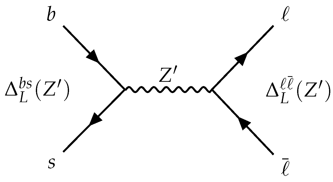
4. FCNC Processes: Effective Hamiltonian in SM and 331 Models

To reconsider the rare FCNC B decays in the framework of 331 models, we recall the SM effective Hamiltonian describing such modes and how it is modified in the 331 case. Specifically, we are concerned with $b\to s{\ell }^{+}{\ell }^{-}$ and $b\to s\nu \overline{\nu }$ modes. The contribution from the tree level $Z^{\prime }$ exchange is depicted in Figure 2.

In SM the effective Hamiltonian governing $b\to s{\ell }^{+}{\ell }^{-}$ reads [33]:

$$\begin{array}{c}\hfill {\mathcal{H}}_{b\to s{\ell }^{+}{\ell }^{-}}^{\mathrm{SM},\mathrm{eff}}=-4\frac{G_F}{\sqrt{2}}{V}_{tb}{V}_{ts}^{*}\left\{C_1{O}_1+C_2{O}_2+\sum _{i=3,\dots ,6}{C}_i{O}_i+\sum _{i=7,\dots ,10}{C}_i{O}_i\right\}+\mathrm{h}.\mathrm{c}..\end{array}$$

(28)

Doubly Cabibbo suppressed terms proportional to $V_{ub}{V}_{us}^{*}$ have been neglected.

$O_1$ and $O_2$ are current-current operators,

$$\begin{array}{cc}\hfill O_1& =\left({\overline{c}}_{\alpha }{\gamma }_{\mu }{P}_L{b}_{\beta }\right)\left({\overline{s}}_{\beta }{\gamma }^{\mu }{P}_L{c}_{\alpha }\right),\hfill \end{array}$$

(29a)

$$\begin{array}{cc}\hfill O_2& =\left(\overline{c}{\gamma }_{\mu }{P}_{L}b\right)\left(\overline{s}{\gamma }^{\mu }{P}_{L}c\right),\hfill \end{array}$$

(29b)

$O_i$$(i=3,\dots ,6)$ are QCD penguins,

$$\begin{array}{cc}\hfill O_3& =\left(\overline{s}{\gamma }^{\mu }{P}_{L}b\right)\sum _q\left(\overline{q}{\gamma }^{\mu }{P}_{L}q\right),O_4=\left({\overline{s}}_{\alpha }{\gamma }^{\mu }{P}_L{b}_{\beta }\right)\sum _q\left({\overline{q}}_{\beta }{\gamma }^{\mu }{P}_L{q}_{\alpha }\right),\hfill \end{array}$$

(30a)

$$\begin{array}{cc}\hfill O_5& =\left(\overline{s}{\gamma }^{\mu }{P}_{L}b\right)\sum _q\left(\overline{q}{\gamma }^{\mu }{P}_{R}q\right),O_6=\left({\overline{s}}_{\alpha }{\gamma }^{\mu }{P}_L{b}_{\beta }\right)\sum _q\left({\overline{q}}_{\beta }{\gamma }^{\mu }{P}_R{q}_{\alpha }\right).\hfill \end{array}$$

(30b)

In (29) and (30) ${\displaystyle P_{R,L}=\frac{1\pm {\gamma }_5}{2}}$ denote the helicity projectors, $\alpha$ and $\beta$ are colour indices. The sum in (30) runs over the flavours $q=\{u,d,s,c,b\}$. The magnetic penguin operators are

$$\begin{array}{cc}\hfill O_7& =\frac{e}{16{\pi }^2}\left[\overline{s}{\sigma }^{\mu \nu }(m_s{P}_L+m_b{P}_R)b\right]F_{\mu \nu },\hfill \end{array}$$

(31)

$$\begin{array}{cc}\hfill O_8& =\frac{g_s}{16{\pi }^2}\left[{\overline{s}}_{\alpha }{\sigma }^{\mu \nu }{\left(\frac{{\lambda }^a}{2}\right)}_{\alpha \beta }(m_s{P}_L+m_b{P}_R)b_{\beta }\right]G_{\mu \nu }^a,\hfill \end{array}$$

(32)

and the semileptonic electroweak penguin operators

$$\begin{array}{cc}\hfill O_9& =\frac{e^2}{16{\pi }^2}\left(\overline{s}{\gamma }^{\mu }{P}_{L}b\right)(\overline{\ell }{\gamma }_{\mu }\ell ),\hfill \end{array}$$

(33)

$$\begin{array}{cc}\hfill O_{10}& =\frac{e^2}{16{\pi }^2}\left(\overline{s}{\gamma }^{\mu }{P}_{L}b\right)(\overline{\ell }{\gamma }_{\mu }{\gamma }_5\ell ).\hfill \end{array}$$

(34)

In previous equations ${\lambda }^a$ are Gell-Mann matrices, $F_{\mu \nu }$ and $G_{\mu \nu }^a$ the electromagnetic and the gluonic field strength tensors, respectively, e and $g_s$ the electromagnetic and strong coupling constants. $m_{b\left(s\right)}$ is the $b\left(s\right)$ quark mass.

The most important operators for $b\to s{\ell }^{+}{\ell }^{-}$ modes are $O_9$ and $O_{10}$. In general new physics (NP) scenarios other operators can be present, such as those with opposite chirality or those with a different Dirac structure, scalar, pseudoscalar or tensor operators. In 331 models the tree-level $Z^{\prime }$ exchange leads to a modification of the values of the Wilson coefficients $C_{9,10}$:

$$\begin{array}{cc}\hfill C_9^{\mathrm{NP}}& =C_9^{\mathrm{SM}}+C_9^{331},\hfill \end{array}$$

(35)

$$\begin{array}{cc}\hfill C_{10}^{\mathrm{NP}}& =C_{10}^{\mathrm{SM}}+C_{10}^{331},\hfill \end{array}$$

(36)

where [5]

$$\begin{array}{cc}\hfill {\sin }^2{\theta }_W{C}_9^{331}& =-\frac{1}{g_{\mathrm{SM}}^2{M}_{Z^{\prime }}^2}\frac{{\Delta }_L^{sb}\left(Z^{\prime }\right){\Delta }_V^{\mu \overline{\mu }}\left(Z^{\prime }\right)}{V_{tb}{V}_{ts}^{*}},\hfill \end{array}$$

(37)

$$\begin{array}{cc}\hfill {\sin }^2{\theta }_W{C}_{10}^{331}& =-\frac{1}{g_{\mathrm{SM}}^2{M}_{Z^{\prime }}^2}\frac{{\Delta }_L^{sb}\left(Z^{\prime }\right){\Delta }_A^{\mu \overline{\mu }}\left(Z^{\prime }\right)}{V_{tb}{V}_{ts}^{*}}.\hfill \end{array}$$

(38)

In previous equations the couplings to leptons are defined as

$$\begin{array}{c}\hfill {\Delta }_{V,A}^{\mu \overline{\mu }}\left(Z^{\prime }\right)={\Delta }_R^{\mu \overline{\mu }}\left(Z^{\prime }\right)\pm {\Delta }_L^{\mu \overline{\mu }}\left(Z^{\prime }\right),\end{array}$$

(39)

where ${\Delta }_L^{sb}\left(Z^{\prime }\right)$ and ${\Delta }_{R,L}^{\mu \overline{\mu }}\left(Z^{\prime }\right)$ are given in Equations (6) and (7).

The real (imaginary) parts of $C_9^{331}$ and $C_{10}^{331}$ separately depend on the parameters of the model but the ratio $C_9^{331}/C_{10}^{331}$, it is independent of the parameters ${\tilde{s}}_{13}$, ${\tilde{s}}_{23}$, ${\delta }_1$, ${\delta }_2$ and $M_{Z^{\prime }}$ [9]. In fact, it only depends on the model variant, and if no $Z-Z^{\prime }$ mixing is considered, its expression reads:

$$\begin{array}{c}\hfill \frac{C_9^{331}}{C_{10}^{331}}=\frac{\mathrm{Re}\left(C_9^{331}\right)}{\mathrm{Re}\left(C_{10}^{331}\right)}=\frac{\mathrm{Im}\left(C_9^{331}\right)}{\mathrm{Im}\left(C_{10}^{331}\right)}=-\frac{\left(\sqrt{3}+9\beta \right){\sin }^2{\theta }_W-\sqrt{3}}{\left(\sqrt{3}-3\beta \right){\sin }^2{\theta }_W-\sqrt{3}}.\end{array}$$

(40)

For the four variant in the analysis, without considering $Z-Z^{\prime }$ mixing, the ratio in (40) has the numerical values:

$$\begin{array}{c}\hfill \frac{C_9^{331}}{C_{10}^{331}}=\left\{\begin{array}{c}-8.874\left(M_1\right)\hfill \\ -2.984\left(M_3\right)\hfill \\ -0.004\left(M_5\right)\hfill \\ +0.595\left(M_7\right)\hfill \end{array}\right..\end{array}$$

(41)

In the case of the transition $b\to s\nu \overline{\nu }$, the SM effective Hamiltonian has a simpler structure deriving from penguin and box diagrams [33]. It consists of a single operator

$$\begin{array}{c}\hfill {\mathcal{H}}_{b\to s\nu \overline{\nu }}^{\mathrm{SM},\mathrm{eff}}=C_L^{\mathrm{SM}}(b,s)O_L+\mathrm{h}.\mathrm{c}.,\end{array}$$

(42)

with

$$\begin{array}{cc}\hfill O_L& =\left(\overline{s}{\gamma }^{\mu }{P}_{L}b\right)\left(\overline{\nu }{\gamma }_{\mu }{P}_L\nu \right).\hfill \end{array}$$

(43)

The SM coefficient $C_L^{\mathrm{SM}}(b,s)$ depends on the quarks in the initial and in the final state:

$$\begin{array}{cc}\hfill C_L^{\mathrm{SM}}(b,s)& =g_{\mathrm{SM}}^2\sum _{U=u,c,t}{V}_{Ub}{V}_{Us}^{*}X\left(x_U\right),\hfill \end{array}$$

(44)

with $g_{\mathrm{SM}}^2$ defined in (22) and $X\left(x_q\right)$ the Inami-Lim function depending on the ratio $x_q=m_q^2/M_W^2$ [34]. The dominant contribution comes from the virtual contribution of the top quark and produces

$$\begin{array}{cc}\hfill \left|C_L^{\mathrm{SM}}(b,s)\right|& \simeq \mathcal{O}\left({10}^{-8}\right).\hfill \end{array}$$

(45)

In this case, the impact of NP could be a modification of the value of $C_L^{\mathrm{SM}}(b,s)$ or the presence of another operator with opposite chirality of the quark current. In 331 models one has

$$\begin{array}{c}\hfill X\left(x_t\right)\to X\left(B_q\right)=X\left(x_t\right)+\frac{1}{g_{\mathrm{SM}}^2{M}_{Z^{\prime }}^2}\frac{{\Delta }_L^{sb}\left(Z^{\prime }\right){\Delta }_L^{\nu \overline{\nu }}\left(Z^{\prime }\right)}{V_{tb}{V}_{ts}^{*}},\end{array}$$

(46)

and the NP coefficient becomes

$$\begin{array}{c}\hfill C_L^{\mathrm{NP}}(b,s)=C_L^{\mathrm{SM}}(b,s)+C_L^{331}(b,s),\end{array}$$

(47)

where [4]

$$\begin{array}{c}\hfill C_L^{331}(b,s)=\frac{{\Delta }_L^{sb}\left(Z^{\prime }\right){\Delta }_L^{\nu \overline{\nu }}\left(Z^{\prime }\right)}{M_{Z^{\prime }}^2}.\end{array}$$

(48)

We can notice that all the coefficients $C_i^{331}$, with $i=\{9,10,L\}$, expressed in Equations (37), (38) and (48) and used in the analyses, depend on $1/M_{Z^{\prime }}^2$. Possible enhancements can be observed if $Z^{\prime }$ is not too heavy. Consequently, we set three values for $M_{Z^{\prime }}$ experimentally accessible at the present facilities: $M_{Z^{\prime }}=\{3,5,7\}\mathrm{TeV}$ with an uncertainty of $5\%$. In the next Section we consider selected FCNC observables that depend on these coefficients within 331 models.

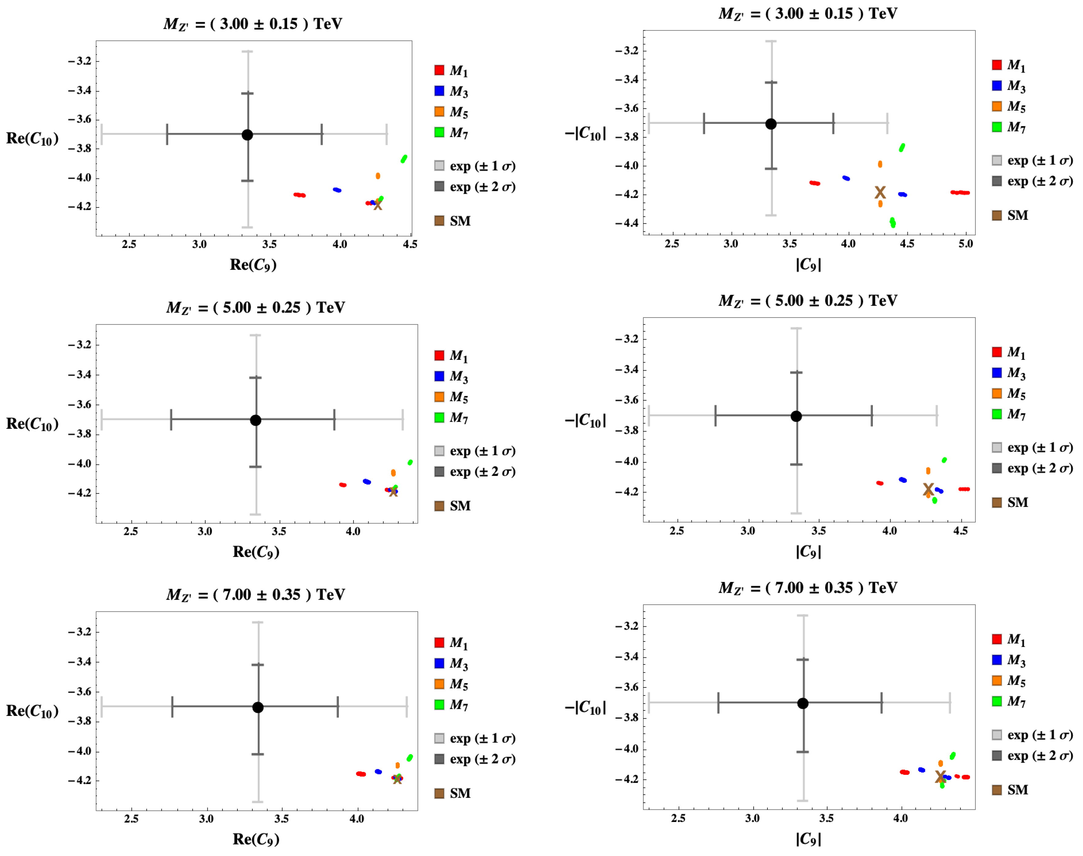
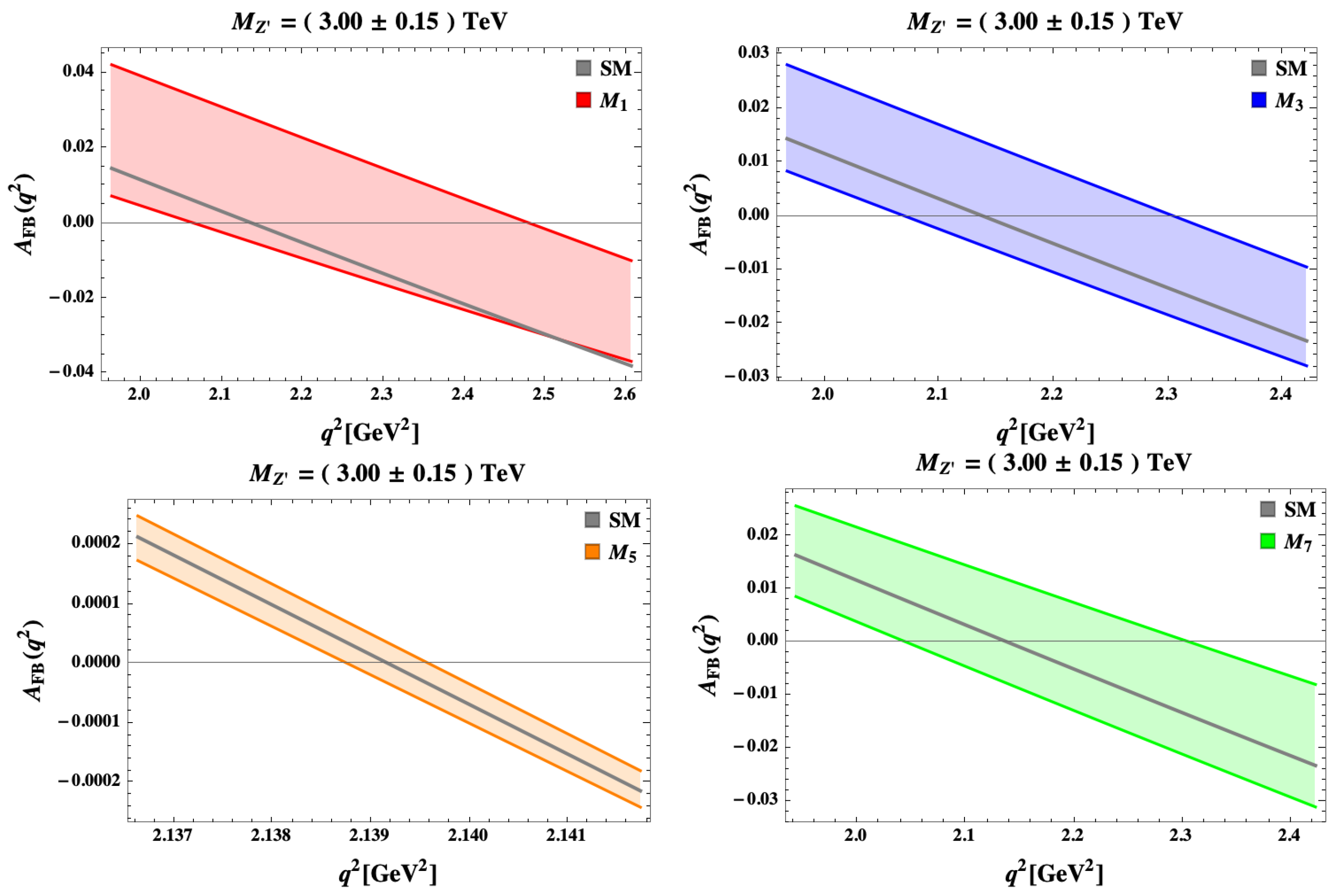
5. The 331 Models Facing New Data on Selected Observables in $\mathit{b}\to \mathit{s}$ Processes

5.1. $b\to s{\ell }^{+}{\ell }^{-}$

A recent study of the LHCb collaboration [35] has provided the values of the Wilson coefficients $C_9^{(\prime )}$ and $C_{10}^{(\prime )}$ fitted from the amplitude analysis of the mode $B^0\to K^{0*}{\mu }^{+}{\mu }^{-}$. It is interesting to consider how 331 models face these new experimental data. According to [35], no sensitivity to the imaginary part of the Wilson coefficients can be achieved treating simultaneously $B^0$ and ${\overline{B}}^0$ decays, so that all coefficients are assumed to be real. Since in 331 models the coefficients do have an imaginary part, we compare the LHCb findings both to the real part of $C_{9,10}$, both to their moduli. In this way we can also appreciate the role of the imaginary part. The results are displayed in Figure 3, comparing the real parts of the coefficients to data in the plots in the left column and their moduli in plots in the right column. Both the SM and 331 models can reproduce the data at $2\sigma$. In particular, the model $M_1$ can reproduce the data with a confidence level of about $1\sigma$, for $M_{Z^{\prime }}\simeq 3\mathrm{TeV}$. Also for the other values of $M_{Z^{\prime }}$, $M_1$ is the variant that performs better on the basis of these observables alone.

For $B\to K^{*}{\mu }^{+}{\mu }^{-}$ another observable can be considered, the forward-backward asymmetry $A_{\mathrm{FB}}\left(q^2\right)$

$$\begin{array}{c}\hfill A_{\mathrm{FB}}\left(q^2\right)=\left[{\int }_0^1\mathrm{d}\cos \theta \frac{{\mathrm{d}}^2\Gamma }{\mathrm{d}{q}^2\mathrm{d}\cos \theta }-{\int }_{-1}^0\mathrm{d}\cos \theta \frac{{\mathrm{d}}^2\Gamma }{\mathrm{d}{q}^2\mathrm{d}\cos \theta }\right]/\frac{\mathrm{d}\Gamma }{\mathrm{d}{q}^2},\end{array}$$

(49)

where $\theta$ is the angle between the positive charged muon and the B meson in the ${\mu }^{+}{\mu }^{-}$ pair rest frame, and $q^2$ is the invariant mass of the muon pair [36,37]. In SM this observable has a zero, a value $q^2=s_0$ such that $A_{\mathrm{FB}}\left(s_0\right)=0$. The value of $s_0$ is almost independent of the model chosen for the form factors [37], so it represents a clean observable to probe possible NP contribution. We consider the model proposed in [38] neglecting the form factors uncertainties. There are NP scenarios that predict either that there is no zero, or that it is displaced with respect to SM. $s_0$ is defined by the relation:

$$\begin{array}{cc}\hfill & \left|C_7\right|\cos \mathrm{Arg}\left(C_{10}\right)m_b\left\{(M_B-M_{K^{*}})V\left(s_0\right)T_2\left(s_0\right)+2(M_B+M_{K^{*}})A_1\left(s_0\right)T_1\left(s_0\right)\right\}+\hfill \\ \hfill & +\left|C_9\right|\cos \left[\mathrm{Arg}\left(C_{10}\right)-\mathrm{Arg}\left(C_9\right)\right]2s_{0}V\left(s_0\right)A_1\left(s_0\right)=0,\hfill \end{array}$$

(50)

and the value in SM is $s_0=2.1392{\mathrm{GeV}}^2$ [38]. The functions V, $A_1$, $T_1$ and $T_2$ in (50) are form factors that parametrize the $B\to K^{*}$ matrix element of the operators in the effective Hamiltonian. Their definition can be found in Appendix A. Indeed, since we are interested in the position of the zero that has a reduced dependence on the form factors, this assumption makes more transparent the comparison with 331 models where the location of the zero is more uncertain due to the variation of the parameters within their allowed ranges. Figure 4 shows the results for this observable in full range of $q^2$, comparing the SM prediction (depicted in gray) to the four considered 331 variants. The range of $q^2$ close to the zero is enlarged in Figure 5, Figure 6 and Figure 7 since the overlap among the curves in Figure 4 does not allow to appropriately distinguish them. It can be observed that, except for $M_5$, in all variants a shift with respect to SM is possible. The largest deviations are found in $M_1$. The results are in

Table 2. Ranges of the zero $s_0$ of the forward-backward asymmetry in $B\to K^{*}{\mu }^{+}{\mu }^{-}$ in the four variants of the 331 models considered in this paper.

${\mathit{M}}_{{\mathit{Z}}^{\prime }}$ (TeV)	$3.00\pm 0.15$	$5.00\pm 0.25$	$7.00\pm 0.35$
$M_1$	$s_0\in [2.0677,2.4821]{\mathrm{GeV}}^2$	$s_0\in [2.1181,2.3325]{\mathrm{GeV}}^2$	$s_0\in [2.1089,2.2798]{\mathrm{GeV}}^2$
$M_3$	$s_0\in [2.0708,2.3059]{\mathrm{GeV}}^2$	$s_0\in [2.1051,2.2410]{\mathrm{GeV}}^2$	$s_0\in [2.1174,2.2112]{\mathrm{GeV}}^2$
$M_5$	$s_0\in [2.1388,2.1396]{\mathrm{GeV}}^2$	$s_0\in [2.1390,2.1394]{\mathrm{GeV}}^2$	$s_0\in [2.1391,2.1394]{\mathrm{GeV}}^2$
$M_7$	$s_0\in [2.0447,2.3075]{\mathrm{GeV}}^2$	$s_0\in [2.0821,2.1965]{\mathrm{GeV}}^2$	$s_0\in [2.0965,2.1748]{\mathrm{GeV}}^2$

.

5.2. $b\to s\nu \overline{\nu }$

The processes $B\to K^{(\ast )}\nu \overline{\nu }$ are theoretically clean. In the SM, their branching ratios are predicted [39]

$$\begin{array}{cc}\hfill \mathcal{B}{(B^{+}\to K^{+}\nu \overline{\nu })}_{\mathrm{SM}}& =(5.22\pm 0.15\pm 0.28)\times {10}^{-6},\hfill \end{array}$$

(51)

$$\begin{array}{cc}\hfill \mathcal{B}{(B^{+}\to K^{*+}\nu \overline{\nu })}_{\mathrm{SM}}& =(11.27\pm 1.38\pm 0.62)\times {10}^{-6},\hfill \end{array}$$

(52)

updating previous results [40,41,42,43,44]. On the other hand, due to the neutrino pair in the final state, they are experimentally challenging. Recently, the Belle II collaboration has provided the measurement [45]:

$$\begin{array}{c}\hfill \mathcal{B}{(B^{+}\to K^{+}\nu \overline{\nu })}_{\exp }=(2.7\pm 0.5\left(\mathrm{stat}\right)\pm 0.5\left(\mathrm{syst}\right))\times {10}^{-5}\end{array}$$

(53)

displaying a tension with the SM result (51). This tension has already triggered a number of analyses [46,47,48,49,50,51,52].

Considering the 331 models, the branching ratio reads

$$\begin{array}{c}\hfill \mathcal{B}{(B^{+}\to K^{+}\nu \overline{\nu })}_{\mathrm{NP}}={\left|\frac{C_L^{\mathrm{NP}}(b,s)}{C_L^{\mathrm{SM}}(b,s)}\right|}^2\mathcal{B}{(B^{+}\to K^{+}\nu \overline{\nu })}_{\mathrm{SM}}.\end{array}$$

(54)

Using the results (51) and (53) in Equation (54), we find that, to reproduce the data, the NP contribution should enhance $C_L^{\mathrm{NP}}(b,s)$,

$$\begin{array}{c}\hfill \left|\frac{C_L^{\mathrm{NP}}(b,s)}{C_L^{\mathrm{SM}}(b,s)}\right|\simeq 2.3\pm 0.3,\end{array}$$

(55)

a relation not satisfied in 331 models, as argued from Figure 8.

In

Table 3. Enhancement of $C_L^{\mathrm{NP}}(b,s)$ for processes mediated by $b\to s\nu \overline{\nu }$ transition in the 331 variants considered in this study with respect to SM prediction. Comparison to the results in [4,10] is also provided.

$|{\mathit{C}}_{\mathit{L}}^{\mathbf{NP}}(\mathit{b},\mathit{s})/{\mathit{C}}_{\mathit{L}}^{\mathbf{SM}}(\mathit{b},\mathit{s}){|}^2$
${\mathit{M}}_{{\mathit{Z}}^{\prime }}$ (TeV)	$\mathbf{3.00}\pm \mathbf{0.15}$		$\mathbf{5.00}\pm \mathbf{0.25}$		$\mathbf{7.00}\pm \mathbf{0.35}$
Variants	[4,10]	Our Result	[4,10]	Our Result	[4,10]	Our Result
$M_1$	$1.003\pm 0.105$	$1.090\pm 0.024$	$1.001\pm 0.063$	$1.047\pm 0.020$	$1.001\pm 0.046$	$1.028\pm 0.022$
$M_3$	$1.001\pm 0.067$	$1.049\pm 0.021$	$1.000\pm 0.040$	$1.024\pm 0.020$	$1.000\pm 0.029$	$1.017\pm 0.015$
$M_5$	$1.000\pm 0.033$	$1.022\pm 0.013$	$1.000\pm 0.020$	$1.011\pm 0.011$	$1.000\pm 0.014$	$1.008\pm 0.008$
$M_7$	$1.000\pm 0.021$	$1.013\pm 0.009$	$1.000\pm 0.013$	$1.008\pm 0.006$	$1.000\pm 0.009$	$1.005\pm 0.005$

we compare our results to those obtained in [4,10].

The new results decrease as the mass $M_{Z^{\prime }}$ increases but not as fast as in the previous analyses. In addition, the values are always larger than 1 at $1\sigma$ level. If further measurements of $\mathcal{B}(B^{+}\to K^{+}\nu \overline{\nu })$ will confirm the Belle II result (53) one should conclude that 331 models are not able to reproduce such data.

6. Conclusions

The important role played by FCNC processes in the search for BSM physics is due to their sensitivity to the virtual contributions of heavy particle exchanges. Exclusive processes such as the purely leptonic $B_s\to {\mu }^{+}{\mu }^{-}$ and the semileptonic ones $B\to K^{(\ast )}{\ell }^{+}{\ell }^{-}$, with $\ell =e,\mu$, allow to investigate possible effects of BSM through several observables.

In this analysis we have considered the 331 models, based on a larger gauge group which includes the SM one. In such models, FCNC processes are mediated by a new heavy neutral gauge boson $Z^{\prime }$ tree-level exchange.

A new approach has been used to constrain the set of the 331 parameters which enter in the observables relative to $B\to K^{*}{\mu }^{+}{\mu }^{-}$ and $B\to K^{(\ast )}\nu \overline{\nu }$. Among the possible 24 models, only four have been selected, showing that for the first process 331 models can perform better than SM. On the other hand, for the modes with neutrinos in the final state, the most recent experimental result are in contention both with SM and 331 models.

References

1. Amhis, Y.; Banerjee, S.; Ben-Haim, E.; Bertholet, E.; Bernlochner, F.U.; Bona, M.; Bozek, A.; Bozzi, C.; Brodzicka, J.; Chobanova, V.; et al. Averages of b-hadron, c-hadron, and τ-lepton properties as of 2021. Phys. Rev. D 2023, 107, 052008. [Google Scholar] [CrossRef]
2. Pisano, F.; Pleitez, V. An SU(3) ⊗ U(1) model for electroweak interactions. Phys. Rev. D 1992, 46, 410–441. [Google Scholar] [CrossRef] [PubMed]
3. Frampton, P.H. Chiral dilepton model and the flavor question. Phys. Rev. Lett. 1992, 69, 2889–2891. [Google Scholar] [CrossRef]
4. Buras, A.J.; De Fazio, F.; Girrbach, J.; Carlucci, M.V. The Anatomy of Quark Flavour Observables in 331 Models in the Flavour Precision Era. J. High Energy Phys. 2013, 02, 023. [Google Scholar] [CrossRef]
5. Buras, A.J.; De Fazio, F.; Girrbach, J. 331 models facing new b+μ data. J. High Energy Phys. 2014, 02, 112. [Google Scholar] [CrossRef]
6. Buras, A.J.; De Fazio, F.; Girrbach-Noe, J. Z-Z′ mixing and Z-mediated FCNCs in SU(3)C × SU(3)L × U(1)X models. J. High Energy Phys. 2014, 08, 039. [Google Scholar] [CrossRef]
7. Buras, A.J.; De Fazio, F. ε′/ε in 331 Models. J. High Energy Phys. 2016, 03, 010. [Google Scholar] [CrossRef]
8. Buras, A.J.; De Fazio, F. 331 Models Facing the Tensions in ΔF = 2 Processes with the Impact on ε′/ε, Bsμ+μ and BK*μ+μ. J. High Energy Phys. 2016, 08, 115. [Google Scholar] [CrossRef]
9. Buras, A.J.; De Fazio, F. 331 model predictions for rare B and K decays, and ΔF = 2 processes: An update. J. High Energy Phys. 2023, 03, 219. [Google Scholar] [CrossRef]
10. Colangelo, P.; De Fazio, F.; Loparco, F. c ν ¯ transitions of Bc mesons: 331 model facing Standard Model null tests. Phys. Rev. D 2021, 104, 115024. [Google Scholar] [CrossRef]
11. Buras, A.J.; Colangelo, P.; De Fazio, F.; Loparco, F. The charm of 331. J. High Energy Phys. 2021, 10, 021. [Google Scholar] [CrossRef]
12. Oliveira, V.; Pires, C.A.d.S. Flavor changing neutral current processes and family discrimination in 3-3-1 models. J. Phys. G 2023, 50, 115002. [Google Scholar] [CrossRef]
13. Oliveira, V.; Pires, C.A.d. Bounds on quark mixing, MZ′ and Z-Z′ mixing angle from flavor changing neutral processes in a 3-3-1 model. Phys. Lett. B 2023, 846, 138216. [Google Scholar] [CrossRef]
14. Singer, M.; Valle, J.W.F.; Schechter, J. Canonical Neutral Current Predictions From the Weak Electromagnetic Gauge Group SU(3) × U(1). Phys. Rev. D 1980, 22, 738. [Google Scholar] [CrossRef]
15. Blanke, M.; Buras, A.J.; Poschenrieder, A.; Tarantino, C.; Uhlig, S.; Weiler, A. Particle-Antiparticle Mixing, ϵK, ΔΓq, A S L q , ACP(BdψKS), ACP(Bsψϕ) and BXs,dγ in the Littlest Higgs Model with T-Parity. J. High Energy Phys. 2006, 12, 003. [Google Scholar]
16. Herrlich, S.; Nierste, U. Enhancement of the KLKS mass difference by short distance QCD corrections beyond leading logarithms. Nucl. Phys. B 1994, 419, 292–322. [Google Scholar] [CrossRef]
17. Herrlich, S.; Nierste, U. Indirect CP violation in the neutral kaon system beyond leading logarithms. Phys. Rev. D 1995, 52, 6505–6518. [Google Scholar] [CrossRef]
18. Herrlich, S.; Nierste, U. The Complete |ΔS| = 2—Hamiltonian in the next-to-leading order. Nucl. Phys. B 1996, 476, 27–88. [Google Scholar] [CrossRef]
19. Buras, A.J.; Jamin, M.; Weisz, P.H. Leading and Next-to-leading QCD Corrections to ϵ Parameter and B0 B ¯ 0 Mixing in the Presence of a Heavy Top Quark. Nucl. Phys. B 1990, 347, 491–536. [Google Scholar] [CrossRef]
20. Urban, J.; Krauss, F.; Jentschura, U.; Soff, G. Next-to-leading order QCD corrections for the B0B0 mixing with an extended Higgs sector. Nucl. Phys. B 1998, 523, 40–58. [Google Scholar] [CrossRef]
21. Brod, J.; Gorbahn, M. Next-to-Next-to-Leading-Order Charm-Quark Contribution to the CP Violation Parameter ϵK and ΔMK. Phys. Rev. Lett. 2012, 108, 121801. [Google Scholar] [CrossRef] [PubMed]
22. Buras, A.J.; Girrbach, J. Complete NLO QCD Corrections for Tree Level ΔF = 2 FCNC Processes. J. High Energy Phys. 2012, 03, 052. [Google Scholar] [CrossRef]
23. Buras, A.J.; Guadagnoli, D. Correlations among new CP violating effects in ΔF = 2 observables. Phys. Rev. D 2008, 78, 033005. [Google Scholar] [CrossRef]
24. Buras, A.J.; Guadagnoli, D.; Isidori, G. On ϵK Beyond Lowest Order in the Operator Product Expansion. Phys. Lett. B 2010, 688, 309–313. [Google Scholar] [CrossRef]
25. Baudis, L.; Zyla, P.A.; Barnett, R.M.; Beringer, J.; Dahl, O.; Dwyer, D.A.; Groom, D.E.; Lin, C.J.; Lugovsky, K.S.; Pianori, E.; et al. Review of Particle Physics. Prog. Theor. Exp. Phys. 2020, 2020, 083C01. [Google Scholar]
26. Chetyrkin, K.G.; Kuhn, J.H.; Maier, A.; Maierhofer, P.; Marquard, P.; Steinhauser, M.; Sturm, C. Addendum to “Charm and bottom quark masses: An update”. arXiv 2017, arXiv:1710.04249. Addendum in Phys. Rev. D 2017, 96, 116007. [Google Scholar] [CrossRef]
27. Chetyrkin, K.G.; Kuhn, J.H.; Maier, A.; Maierhofer, P.; Marquard, P.; Steinhauser, M.; Sturm, C. Charm and Bottom Quark Masses: An Update. Phys. Rev. D 2009, 80, 074010. [Google Scholar] [CrossRef]
28. Brod, J.; Gorbahn, M.; Stamou, E. Updated Standard Model Prediction for Kπν ν ¯ and ϵK. arXiv 2021, arXiv:2105.02868. [Google Scholar]
29. Aoki, S.; Aoki, Y.; Bečirević, D.; Blum, T.; Colangelo, G.; Collins, S.; Della Morte, M.; Dimopoulos, P.; Dürr, S.; Fukaya, H.; et al. FLAG Review 2019: Flavour Lattice Averaging Group (FLAG). Eur. Phys. J. C 2020, 80, 113. [Google Scholar] [CrossRef]
30. Heavy Flavor Averaging Group (HFLAV); Amhis, Y.; Banerjee, S.; Ben-Haim, E.; Bernlochner, F.; Bozek, A.; Bozzi, C.; Chrząszcz, M.; Dingfelder, J.; Duell, S.; et al. Averages of b-hadron, c-hadron, and τ-lepton properties as of summer 2016. Eur. Phys. J. C 2017, 77, 895. [Google Scholar] [CrossRef]
31. Aoki, Y.; Blum, T.; Colangelo, G.; Collins, S.; Morte, M.D.; Dimopoulos, P.; Dürr, S.; Feng, X.; Fukaya, H.; Golterman, M.; et al. FLAG Review 2021. Eur. Phys. J. C 2022, 82, 869. [Google Scholar] [CrossRef]
32. Dowdall, R.J.; Davies, C.T.H.; Horgan, R.R.; Lepage, G.P.; Monahan, C.J.; Shigemitsu, J.; Wingate, M. Neutral B-meson mixing from full lattice QCD at the physical point. Phys. Rev. D 2019, 100, 094508. [Google Scholar] [CrossRef]
33. Buras, A. Gauge Theory of Weak Decays; Cambridge University Press: Cambridge, UK, 2020. [Google Scholar]
34. Buras, A.J. Weak Hamiltonian, CP violation and rare decays. In Proceedings of the Les Houches Summer School in Theoretical Physics, Session 68: Probing the Standard Model of Particle Interactions, Les Houches, France, 28 July–5 September 1997; Volume 6, pp. 281–539. [Google Scholar]
35. Aaij, R.; Abdelmotteleb, A.S.W.; Beteta, C.A.; Abudinén, F.; Ackernley, T.; Adeva, B.; Adinolfi, M.; Adlarson, P.; Agapopoulou, C.; Aidala, C.A.; et al. Determination of short- and long-distance contributions in B0K*0μ+μ decays. arXiv 2023, arXiv:2312.09102. [Google Scholar]
36. Altmannshofer, W.; Ball, P.; Bharucha, A.; Buras, A.J.; Straub, D.M.; Wick, M. Symmetries and Asymmetries of BK*μ+μ Decays in the Standard Model and Beyond. J. High Energy Phys. 2009, 01, 019. [Google Scholar] [CrossRef]
37. Beneke, M.; Feldmann, T. Symmetry breaking corrections to heavy to light B meson form-factors at large recoil. Nucl. Phys. 2001, B592, 3–34. [Google Scholar] [CrossRef]
38. Ball, P.; Zwicky, R. Bd,sρ, ω, K*, ϕ decay form-factors from light-cone sum rules revisited. Phys. Rev. 2005, D71, 014029. [Google Scholar]
39. Bečirević, D.; Piazza, G.; Sumensari, O. Revisiting BK(*)ν ν ¯ decays in the Standard Model and beyond. Eur. Phys. J. C 2023, 83, 252. [Google Scholar] [CrossRef]
40. Colangelo, P.; De Fazio, F.; Santorelli, P.; Scrimieri, E. Rare BK(*) neutrino anti-neutrino decays at B factories. Phys. Lett. B 1997, 395, 339–344. [Google Scholar] [CrossRef]
41. Buras, A.J.; Girrbach-Noe, J.; Niehoff, C.; Straub, D.M. BK(*)ν ν ¯ decays in the Standard Model and beyond. J. High Energy Phys. 2015, 02, 184. [Google Scholar] [CrossRef]
42. Altmannshofer, W.; Buras, A.J.; Straub, D.M.; Wick, M. New strategies for New Physics search in BK*ν ν ¯ , B ν ¯ and BXsν ν ¯ decays. J. High Energy Phys. 2009, 04, 022. [Google Scholar] [CrossRef]
43. Blake, T.; Lanfranchi, G.; Straub, D.M. Rare B Decays as Tests of the Standard Model. Prog. Part. Nucl. Phys. 2017, 92, 50–91. [Google Scholar] [CrossRef]
44. Parrott, W.G.; Bouchard, C.; Davies, C.T.H.; Hpqcd Collaboration. Standard Model predictions for BKℓ+, BK 1 2 + and B ν ¯ using form factors from Nf = 2 + 1 + 1 lattice QCD. Phys. Rev. D 2023, 107, 014511. [Google Scholar] [CrossRef]
45. Adachi, I.; Adamczyk, K.; Aggarwal, L.; Ahmed, H.; Aihara, H.; Akopov, N.; Aloisio, A.; Ky, N.A.; Asner, D.M.; Atmacan, H.; et al. Evidence for B+K+ν ν ¯ Decays. arXiv 2023, arXiv:2311.14647. [Google Scholar]
46. Bause, R.; Gisbert, H.; Hiller, G. Implications of an enhanced B ν ¯ branching ratio. arXiv 2023, arXiv:2309.00075. [Google Scholar] [CrossRef]
47. Allwicher, L.; Becirevic, D.; Piazza, G.; Rosauro-Alcaraz, S.; Sumensari, O. Understanding the first measurement of B(B ν ¯ ). Phys. Lett. B 2024, 848, 138411. [Google Scholar] [CrossRef]
48. He, X.-G.; Ma, X.-D.; Valencia, G. Revisiting models that enhance B+K+ν ν ¯ in light of the new Belle II measurement. arXiv 2023, arXiv:2309.12741. [Google Scholar]
49. Berezhnoy, A.; Melikhov, D. BK*MX vs BKMX as a probe of a scalar-mediator dark matter scenario. arXiv 2023, arXiv:2309.17191. [Google Scholar]
50. Datta, A.; Marfatia, D.; Mukherjee, L. B ν ¯ , MiniBooNE and muon g-2 anomalies from a dark sector. arXiv 2023, arXiv:2310.15136. [Google Scholar] [CrossRef]
51. McKeen, D.; Ng, J.N.; Tuckler, D. Higgs Portal Interpretation of the Belle II B+K+νν Measurement. arXiv 2023, arXiv:2312.00982. [Google Scholar]
52. Fridell, K.; Ghosh, M.; Okui, T.; Tobioka, K. Decoding the BKνν excess at Belle II: Kinematics, operators, and masses. arXiv 2023, arXiv:2312.12507. [Google Scholar]
Figure 1. Allowed ranges for δ 1 and δ 2 . The blue (green) region is obtained using the conditions on the observables relative to the B d ( B s ) system. The red region is the intersection of those regions, while the gray one is obtained taking into account also the constraints from the observables in the K system.
Particles 07 00009 g001
Figure 2. Feynman diagram for b s ¯ transition mediated by Z in the 331 models, with = { μ , ν } .
Particles 07 00009 g002
Figure 3. Correlation plot between Wilson coefficients C 9 and C 10 for three selected ranges of M Z . The plots on the left are obtained assuming that C 9 , 10 are real, as assumed in [35], while those on the right take into account the possibility that they have an imaginary part. The gray bars correspond to the experimental results in [35] taken at 1 σ and 2 σ level, while the brown cross represents the SM prediction. The other points corresponding to different 331 variants (different values of the parameter β ) are distinguished by the colours: red ( M 1 ), blue ( M 3 ), orange ( M 5 ) and green ( M 7 ).
Particles 07 00009 g003
Figure 4. Forward-backward asymmetry (49). The SM prediction (gray curve) is compared to the four considered 331 models and M Z 3 TeV (left), M Z 5 TeV (middle) and M Z 7 TeV (right panel). For M i models, the legend is the same as in Figure 3.
Particles 07 00009 g004
Figure 5. Zoom of the region close to the zero of the forward-backward asymmetry (49) for B K * μ + μ . The SM prediction is compared to M 1 (top-left), M 3 (top-right), M 5 (bottom-left) and M 7 (bottom-right) in the case M Z 3 TeV . Same legend as in Figure 4.
Particles 07 00009 g005
Figure 6. Zoom of the region close to the zero of the forward-backward asymmetry (49) for B K * μ + μ . The SM prediction is compared to M 1 (top-left), M 3 (top-right), M 5 (bottom-left) and M 7 (bottom-right) in the case M Z 5 TeV . Same legend as in Figure 4.
Particles 07 00009 g006
Figure 7. Zoom of the region close to the zero of the forward-backward asymmetry (49) for B K * μ + μ . The SM prediction is compared to M 1 (top-left), M 3 (top-right), M 5 (bottom-left) and M 7 (bottom-right) in the case M Z 7 TeV . Same legend as in Figure 4.
Particles 07 00009 g007
Figure 8. Branching ratio B ( B + K + ν ν ¯ ) . Experimental data (gray line) and SM prediction (brown line) are compared to the four different 331 models considered in this study. Same legend as in Figure 4.
Particles 07 00009 g008