Abstract
Axions can be considered as good dark matter candidates. The detection of such light particles can be achieved by observing axion-induced atomic excitations. The target is in a magnetic field so that the m-degeneracy is removed, and the energy levels can be suitably adjusted. Using an axion-electron coupling indicated by the limit obtained by the Borexino experiment, which is quite stringent, reasonable axion absorption rates have been obtained for various atomic targets The obtained results depend, of course, on the atom considered through the parameters (the spin−orbit splitting) as well as ( the energy splitting due to the magnetic moment interaction). This assumption allows axion masses in the tens of eV if the transition occurs between members of the same multiplet, i.e., , and axion masses in the range 1 meV–1 eV for transitions of the spin−orbit splitting type , i.e., three types of transition. The axion mass that can be detected is very close to the excitation energy involved, which can vary by adjusting the magnetic field. Furthermore, since the axion is absorbed by the atom, the calculated cross-section exhibits the behavior of a resonance, which can be exploited by experiments to minimize any background events.
Keywords:
axion detection; axion dark matter; atomic excitations; magnetic field induced level splitting; magnetic moment matrix element; narrow resonances; light absorption; frequency and magnetic field scan; event rate PACS:
93.35+d 14.80.-j 14.80.Va 98.35.Gi 21.60.Cs
1. Introduction
In the standard model (S-M) there is a source of CP violation from the phase in the Kobayashi-Maskawa mixing matrix. This, however, is not large enough to explain the baryon asymmetry observed in nature. Another source is the phase in the interaction between gluons (-parameter), naively expected to be of order unity. The non-observation of the elementary electric dipole moment of the neutron limits its value to be . This has been known as the strong CP problem. A solution to this problem has been the P-Q (Peccei-Quinn) mechanism. In extensions of the S-M, e.g., two Higgs doublets, the Lagrangian has a global P-Q chiral symmetry , which is spontaneously broken, generating a Goldstone boson, the axion (a). In fact, the axion was proposed a long time ago as a solution to the strong CP problem [1] resulting in a pseudo-Goldstone boson [2,3]. The two most widely cited models of invisible axions are the KSVZ (Kim, Shifman, Vainshtein, and Zakharov) or hadronic axion models [4,5] and the DFSZ (Dine, Fischler, Srednicki, and Zhitnitskij) or GUT axion model [6,7]. This also led to the interesting scenario of the axion being a candidate for dark matter in the universe [8,9,10] and it can be searched for by real experiments [11,12,13,14]. For a review see, see, e.g., [15].
It has been recognized a long time ago by Sikivie [16], and others, see, e.g., [17], that the axion is an ideal cold dark matter candidate, especially in the mass range eV eV. Thus, popular experiments hope to detect axions by their conversion to photons in the presence of a magnetic field (Primakoff effect); see Figure 1a,b. The produced photons are detected in a resonance cavity as suggested by Sikivie [16]. In the case of the axion absorption by atoms, see Figure 1c, the detection can be achieved by directly measuring the photons following the atom de-excitation or by promoting the axion to a judiciously chosen third level via suitable light absorption, with a desired pattern of de-excitation as described below.
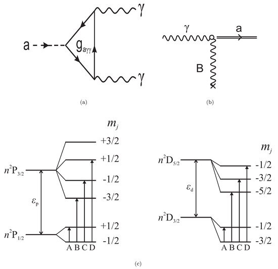
Figure 1.
(a) The elementary axion-photon interaction. (b) The axion to photon conversion in the presence of a magnetic field, the Primakoff effect. (c) The axion absorption by an atom at low temperature via the axion-electron spin-induced interaction. An example of transitions is indicated. The energy splittings depend on the spin-orbit interaction and the magnitude of the magnetic field (the levels are not to scale). An electron is moved from an occupied initial level with energy and quantum numbers in the substate to a level with energy with quantum numbers , provided that , consistent with the angular momentum selection rules (terms B,C,D). When the total angular momentum of the two states is the same (A-term), the splitting is small and due to the magnetic moment operator. In all cases, the splitting is proportional to the magnetic field. The picture is drawn for one-electron configurations, but it can be generalized to multi-electron configurations. In all cases, only states with the same radial and orbital quantum numbers can be connected via the spin operator.
In fact, various experiments (heavier axions with larger mass in the 1eV region produced thermally (such as via the mechanism), e.g., in the sun, are also interesting and are searched by CERN Axion Solar Telescope (CAST) [18]. Other axion-like particles (ALPs), with broken symmetries not connected to QCD, and dark photons form dark matter candidates called WISPs (Weakly Interacting Slim Particles), see, e.g., [19], are also being searched) such as the ADMX and the ADMX-HF collaborations [11,13,20,21] are planned and ongoing to search for them. In addition, the newly established Center for Axion and Physics Research (CAPP) has started an ambitious axion dark matter research program [22], using SQUID and HFET technologies [23]. Their strategy is to run several experiments in parallel to explore a wide range of axion masses with sensitivities better than the QCD axion models [24,25,26].
The allowed parameter space has been presented in a nice slide by Raffelt [27] in the Multidark-IBS workshop and, focusing on the axion as dark matter candidate, by Stern [20], derived from Figure 3 of ref. [20].
Recently, some exclusions on the axion masses have been obtained by the ADMX experiments in the range of 2.66–2.81 eV [28], 2.81–3.39 eV [29] and 3.3–4.2 eV [30] leading to the exclusion of a wide range of axion-photon coupling values predicted in benchmark models of the invisible axion, which solves the strong CP problem of quantum chromodynamics.
Since, however, the mass of the axion is not known, it is important to consider other processes for its detection, which may be accessible to a wider window of axion mass. Such may involve, e.g., axion detection via atomic excitations [31,32,33].
In this paper, we are going to discuss the possibility of axion detection by observing directly axion-induced atomic excitations, measuring the photons produced in the de-excitation with sensitivity to axion masses ranging eV and up close to 1 eV. More specifically the relevant procedure, suggested by Sikivie [34], involves an atom cooled at low temperature, which utilizes three energy levels. The first is the ground state, . The second, is completely empty, chosen such that the energy difference between the two is close to the axion mass. Under the spin-induced axion-electron interaction, an electron is excited from the first to the second level. The presence of such an electron in can be confirmed by exciting it further via the radiation of suitably chosen photon energy to a third level , which is also empty and lies at higher excitation energy. From the observation of the subsequent de-excitation of level , one infers the presence of the axion.
The magnetic field employed is used to split the magnetic m-substates so that the transition energies involved can be suitably adjusted. Furthermore, by suitably adjusting its size, it can determine a window of axion masses to be searched in a given experiment.
A crucial parameter in the axion-induced atomic excitations is the axion electron coupling . The dimensionless quantity has been studied in axion models. The quantity with dimension of mass is not known, but it is believed to be inversely proportional to the axion mass. Limits on the axion electron coupling have been extracted from recent astrophysical data [35,36,37]. In the present calculation, we are going to adopt a value , which coincides with the stringent limit obtained in the Borexino experiment [38]. We will see that this value leads to a very small cross-section. Fortunately, we will find that experiments involving dark matter axions are not doomed to be unobservable since the axion number density in our vicinity of the galaxy is quite large, owing to the small axion mass.
Our paper will be organized as follows. In Section 2 we will derive expressions yielding the rates for axion absorption by atoms; in Section 3 we will discuss the axion-electron coupling and the range of the axion masses obtained from Borexino limit in conjunction with reasonable axion model parameters , in Section 4 we will study the obtained axion widths, in Section 5 we will summarize the needed atomic physics input, in Section 6 we will consider the low-temperature requirements for the success of the experiments, in Section 7 we will present our results for the expected rates and in Section 8 we will summarize our conclusions.
2. Expressions for Rates for Axion Absorption by Atoms
We remind the reader that the axion, a, is a pseudoscalar particle, and its coupling to the electron can be described by a Lagrangian of the form:
where is a coupling constant and a scale parameter with the dimension of mass. For an axion with mass it is easy to show that in the non-relativistic limit:
- The time component is given by:which is negligible for .
- The space component, , iswhere and are the initial and final electron momenta, the axion decay constant and the spin of the electron.
An interaction of the form of Equation (3) has been proposed by Sikivie [34] as a way of detecting the axion by causing atomic excitations, with the relevant coupling constant to be determined by the experiment.
The target is selected so that there exist two levels, say and which result from the splitting of the atomic levels by the magnetic field and they are characterized by the same n and ℓ so that they can be connected by the spin operator. Thus or , in which case is the spin-orbit partner of . The lower one is occupied by electrons, but the higher one is completely empty at a sufficiently low temperature, see Figure 1c. can be populated only by exciting an electron to it from the lower level by the axion field. The occurrence of such excitation is monitored by a tuned laser beam, which excites such an electron from to a higher state , which cannot be reached in any other way by observing its subsequent decay.
In the present case we are interested in the case that the states and can be connected via the spin operator, i.e., the two states must have the same orbital structure, and angular momenta (for single-particle states, , , they must have the same n and ℓ quantum numbers). In other words we must evaluate the matrix element , where denotes any additional quantum number needed to specify the states.
As an illustration, let us consider a single particle transition. The relevant matrix element for the transition takes the form
where depends on the atomic levels [39] and it will be given below (see Section 5) and is given by
Since the momentum transfer is small, . It can be shown that a similar result holds in the case of multi-particle configurations. So, the matrix element becomes
where is the momentum transfer to the atom with its component in the direction of the axis of quantization and , along the other two axes.
The cross-section becomes
where the momentum transfer to the atom. is the usual normalization for a boson field. In the above expression, we have neglected the tiny recoiling energy of the atom. Thus:
We will now fold the cross-section with the axion velocity distribution, assuming that with respect to the galactic center it is of the Maxwell–Boltzmann type:
In the local frame, ignoring for the moment the motion of the Earth, we have
This can be cast in the form:
where
or
with
So the integration over the angles yields:
The integration over can be performed analytically yielding
The integration over the magnitude of the velocity is trivial due to the function appearing in Equation (14). We thus obtain:
with X given by
and
The extra factor of in going from Equation (16) to Equation (19) is the result of the integration over the velocity.
Thus, one obtains:
The event rate associated with a flux of particles with velocity (per atom in the target) is given by:
where is the axion flux given by with the axion matter density in our vicinity of the galaxy. In this work, we will assume that all dark matter in our vicinity is composed of axions. So, it is obtained from the rotation curves and employed in standard dark matter searches, i.e., . This leads to a large axion particle density due to the smallness of the axion mass.
Thus Equation (23) for N atoms in the target becomes
is written as a product of two constants, one with the dimension of the flux, which varies inversely proportional to the axion mass, and the other yields the scale of the cross section.
3. The Axion Electron Coupling
A crucial parameter in the present work is . In the past, this parameter was derived from existing axion models. In this work, we are going to consider limits obtained from a robust experiment [38] which are as follows:
These can be interpreted to be the axion-electron and the isovector axion-nucleon coupling, which in our notation are written:
Using now the equation
found in [40,41], we obtain
These couplings are indeed very small. This perhaps explains why for the Borexino 5.5 MeV axion flux on Earth, resulting from the second relation of the equation, is very small. This is the reason why, in our recently published paper [41] we had to admit that the nuclear excitations were not detectable. Anyway, we will assume the equality sign, i.e., the above limits correspond to the actual values of these quantities, and we will employ this electron-axion coupling in the present work.
The coupling is not known. However, it has been investigated [42,43], in particular in the context of the DFSZ axion models [7,9]. This leads to:
where is the ratio of the vacuum expectation values of the two doublets of the model. The parameter is not known.
In the present work, we will assume that the upper limit of Equation (26) corresponds to the actual value of . Then, since the overall coupling in Equation (26) depends on both the axion mass and the coupling , we obtain a range for the axion mass, see Figure 2a. Having such a range of axion masses, it is amusing to note that once the axion mass is determined one can determine the ratio , see Figure 2b.
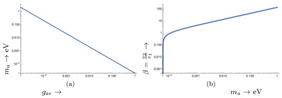
Figure 2.
(a) The axion mass allowed by the coupling given in Equation (26) as a function of . This covers almost the whole range of of interest in this work. (b) The ratio of the expectation values of the Higgs doublets of the DFSZ axion model discussed in the text as a function of the axion mass .
Anyway, from Equation (26), one finds per mol-y. Thus, the main axion mass dependence of the event is as shown in Figure 3. Additional axion mass dependence, which can be exploited by experiment, is contained in through X, see Equation (18).
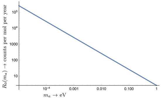
Figure 3.
The main axion mass dependence . This sets the scale of the event rate as a function of the axion mass.
4. The Axion Absorption Widths
Since the axion is absorbed, one expects the cross-section to exhibit a resonant behavior. This is exhibited by considering the function in the variable X, which depends on the energy difference of the atomic levels, the axion mass, and the velocity of the sun around the center of the galaxy. The energy difference depends, of course, on the magnetic quantum numbers and of the states involved.
The overall behavior of the functions is exhibited in Figure 4. In fact, we find that the characteristics of the resonance are:
where is the location of the maximum
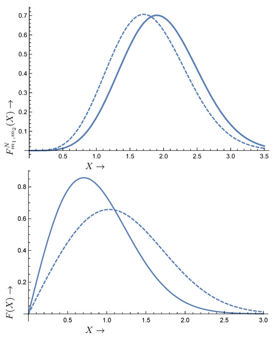
Figure 4.
(Top): The normalized distribution as a function of X, with the velocity of the sun around the center of the galaxy in natural units, . The solid line holds for , while the dashed line for . The widths are the same, , for both cases. The corresponding values of are 1.9 and 1.7 for the solid and dashed curves, respectively. (Bottom): For comparison the normalized distribution , with the photon energy, in the case of the standard axion to photon conversion is presented, as obtained with the same halo parameters as in the top panel, in the galactic frame (solid curve) and local frame (dashed curve).
We have seen that we have resonant behavior in the variable X. At the location of the maximum, from the relation , we find that
For all practical purposes the axion mass is equal to the excitation energy. Furthermore
Similarly, we can find the width in the energy space for both types of transitions. Thus,
and therefore
At , i.e., at , the distribution vanishes. On the other hand at i.e., for , the distribution almost vanishes (there is no need to go to values of , since velocities above the escape velocity, , in the Maxwell–Boltzmann distribution have been excluded). In other words, the distribution vanishes at and at after having gone very rapidly through with a width as given by Equation (33). In any case, the above picture emerges more clearly by plotting the function as a function of the energy , see Figure 5.
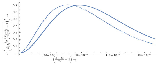
Figure 5.
The cross-section exhibits resonant behavior. Shown is as a function of . The solid line corresponds to , while the dashed line corresponds to , both in the local frame.
We have seen that the axion mass is very close to the excitation energy. Since the resonance is so narrow, however, special care is required not to miss it. Some experimental arrangements to facilitate the observation of such a narrow resonance from the expected atomic spectra will be considered below; see Section 7. Furthermore, to this end, the experience gained with the axion to photon conversion experiments involving resonant cavities, such as ADMX and ADMX-HF collaborations [11,13,20,21] and CAPP [22,23,24,25,26], may be very helpful. For the observation of the resonance, it is very important, among other things, to discriminate against background. It is very unlikely that background events will simulate a similar resonance pattern with that obtained here, reflecting not only the Maxwell–Boltzmann distribution, but the momentum dependence of the axion-electron system as well. Furthermore, given enough counts, one can exploit, if it becomes necessary, the extra signature, provided by the fact that the resonance width exhibits time dependence, i.e., an annual modulation due to the motion of the Earth, see [44] and the Appendix A.
Before completing this section we should mention that resonance plots, correlated with the event rate, will be specialized in Section 7 for the various atomic targets considered in this work.
5. Atomic Physics Considerations
We will now consider some atomic targets which possess two features. The ground state is composed of a multiplet of the form while the excited state is of the form with , so that it can be reached by spin excitations.
The following types of excitations are in principle possible:
- , indicated as type A
- , indicated as type B
- , indicated as type C
- , indicated as type D
As we will see below some of these types may not be allowed by the angular momentum selection rules. Thus, e.g., for states single-particle states only the A type is possible. For many electron configurations see Section 5.2.
5.1. Single-Particle Spin-Orbit Partners
The ground state of a single particle state is of the form while the state is empty. Such examples can be found in the atomic data.
Since this is one body transition, the relevant matrix element takes the form:
i.e., it is simply expressed in terms of a Glebsch–Gordan coefficient and the nine-j symbol. We are interested in the case . The relevant coefficients are tabulated in Table 1.

Table 1.
The coefficients connecting via the spin operator a given initial state with all possible states , for .
(i) First we will consider a target with the ground state being a single orbital, while the is empty. Let us suppose that the spin-orbit splitting is . In the presence of a magnetic field, the m-degeneracy is removed, and the ground state is in the state . Then we have the following spin-induced transitions:
indicated as above, i.e., A, B, C, and D, respectively. The g-factors for the and p-levels are 2/3 and 4/3, respectively. Thus the transition energies (not to be confused with m the magnetic quantum number) are
where we have included both the spin and orbital magnetic moments with with the Bohr magneton and B the magnetic field. For a field of 1T we find eV, i.e.,
A good candidate for such a transition is 13Al, involving the orbitals and . From existing tables (https://www.nist.gov/pml/atomic-spectra-database, accessed on 19 January 2024) we find eV. The spin-induced matrix elements are as follows
(ii) Next we will consider a target with the ground state containing a single orbital, while the is empty. Let us suppose that the spin-orbit splitting is . In the presence of a magnetic field, the m-degeneracy is removed, and the ground state is in the state . Then we have the following spin-induced transitions:
indicated again as A, B, C and D, respectively. The g-factors for the and d-levels are 4/5 and 6/5, respectively. Thus, the excitation energies are:
where we have included both spin and orbital magnetic moment.
Our best candidate found in the above-mentioned reference with the NIST tables is the target 21Sc involving the transitions with eV. Other candidates can also be found in the same reference, e.g., Z = 39 (Y I, eV) and Z = 71 (Lu I, , eV) where I indicates that it is a neutral atom.
Thus, we can use Equation (37) with the appropriate value of and the spin-induced
(iii) states. Such states exist in many atomic targets. In all such cases
We note the relatively large spin matrix for single particle excitations.
Note that, in the case of and the A type transitions, the lowest value of the axion mass required for the process to take place is very small since the spin-orbit splitting does not appear. If such a configuration exists in the ground state of the atom considered, the obtained results are independent of the atom.
The transition energy is also small for the other type of transitions if the spin-orbit splitting is small, e.g., in the case of all 3d-transitions considered here.
5.2. More Than One-Electron Configurations
5.2.1. Two-Electron Configurations
The simplest possible case is two-electron configurations. Now, the needed states are spin-symmetric. The antisymmetry of the wave functions requires the space part to be antisymmetric, i.e., a wave function of the form
i.e., spin triplet and L odd states.
Of special interest are the cases involving the functions:
Then the spin matrix element can be cast in the form:
The is the spin-reduced matrix element, and it can be calculated by techniques familiar to atomic physics.
Good candidates are the following:
(i) .
In this case, the ground state (gs) of the carbon atom is of the form , while the excited state, which can be populated by spin excitations, is 3 at 16.41671 cm−1, about 0.002 eV. It may be useful to note that the silicon atom (Si I) has the same structure, except for the gs radial quantum number and the fact that eV. The radial quantum number does not affect the calculations performed here, while the fine structure splitting can be selected on the basis of the axion mass being searched. That being said, the experimenters can choose whichever is more appropriate for them.
So since in both cases, the initial state is not degenerate, only the excitations caused by the spin operator appear. Furthermore, one needs to consider of the splitting of the final multiplet , which is given by
Thus in the case of carbon
(ii)
A good such candidate is the Ti atom. In this case the gs is of the form . The excited state that can be reached is 3 at 170.134, cm−1 = 0.02 eV. Another good candidate is the neutral Zirconium (Zr I) atom. This has the same structure, except for the radial quantum number being , which is irrelevant for our calculations, and the fact that eV. The latter affects the axion mass to be extracted by the experimenters. So the choice of the target can be selected on the basis of the same criteria as above. Thus, for both cases
including both the spin and the orbital magnetic moment.
The relevant spin matrix element is given in Table 2.
Table 2.
The coefficients , and as well as the corresponding total matrix elements relevant to the present work. Note that the initial sub-state is of the form .
5.2.2. More Than Two-Electron Configurations
(i) The oxygen atom.
In this case, the gs is of the form , while the excited state, which can be populated by spin excitations, is 3 at 158.265 cm−1, about 0.0196 eV. This target is appropriate at the low temperatures we consider since it is no longer a gas. Otherwise, one might consider the atom of Sulfur (S I), which has the same configuration but with instead of . Returning to the oxygen atom, we will consider the splitting of the ground state multiplet , as well as of the final state multiplet
By angular momentum selection rules only the A and the D terms are allowed. Thus one finds
including the contribution of both the spin and orbital magnetic moment.
(ii) The 26Fe atom.
The ground state is of the form , while the excited state that can be populated by spin excitations is the first excited one 5 at 415.933 cm−1 = 0.0516 eV. The calculation of the reduced spin and orbital angular momentum matrix elements is a bit complicated, but it can be simplified by making use of the symmetries of the wave functions. The spin part is characterized by the SU(2) symmetry while antisymmetry requires the orbital part to be under SU(5). The relevant matrix elements can be evaluated using standard techniques, see, e.g., [45], table B.19. Since only the transitions of the type A and D appear in this case, one finds
including both the spin and the orbital magnetic moments.
The needed spin-induced transition matrix elements and and are shown in Table 2.
6. Low Temperature Requirements
As we have mentioned, the detection of very light axions in the regime of a few eV mass crucially depends on the condition that the second level must be essentially free of electrons. To achieve this condition the target material should be brought at cryogenic temperatures. The critical temperature depends on the axion mass to be explored. The ratio of the probabilities of finding an accidental electron in the second level relative to the probability of finding one in the first level is given by the Boltzmann distribution probability:
Suppose that we demand
Then we find that
The condition on the temperature is given in Figure 6.
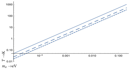
Figure 6.
The temperature in degrees Kelvin to be achieved is the region below the above curves so that the population of the excited state by thermal electrons can be neglected. The continuous curve corresponds to relative probability of , the long dash to and the sort dash to .
We thus see that, for axion mass eV associated with a magnetic field B = 1 T, K may be required. The situation may improve, of course, for larger magnetic fields. Typical laboratory fields, however, are sometimes not sufficiently weak for the Zeeman effect adopted here to apply. If B is typical but strong, either an intermediate case applies or the Paschen–Back effect. Here, throughout the paper it is assumed that the Zeeman effect always applies, but, strictly speaking, this holds only when the B-induced splittings are small as compared to the fine structure ones, say
In particular, when is of the order of meV and the Zeeman corrections are of the order of eV, we are certainly on the safe side. On the other hand for axions heavier than 0.1 eV, truly cryogenic temperatures are not required.
Accidental backgrounds causing the excitation may be rejected from the resonant behavior since it is unlikely that they are going to have a velocity distribution similar to that of the axions in the local frame.
There remains, however, an additional problem. For very light axions, one has to develop target materials, which, at these cryogenic temperatures, exhibit atomic structure. Ordinary atoms do not suffice. One demands that the ions of the crystal still exhibit atomic structure involving the bound electrons, as, e.g., the CUORE detector of Crystalline 130TeO2 at cryogenic temperatures. The electronic states probably will not carry all the important quantum numbers as their corresponding neutral atoms, but they should possess the configurations connected by the spin excitations considered here. So, one may prefer to consider targets that contain appropriate impurity atoms in a host crystal, e.g., chromium in sapphire. As a matter of fact, it is very encouraging that already there exist proposals involving rare-earth ions doped into solid-state crystalline materials [46] at cryogenic temperatures. In fact, if ion impurities are doped in crystals, one has to choose the target atoms in such a way that the corresponding ions can be isoelectronic to the atoms presented here and have the same configurations and terms. Since, as we shall see below, the expected rates for light axions are quite large, small impurities of 1 to 1000 or even 1/10,000 may be adequate, or one may relax the condition on the relative probability , see Equation (44).
It is also possible that one may be able to employ at cryogenic temperatures some exotic materials used in quantum technologies (for a review see [47]) like nitrogen-vacancy (NV), i.e., materials characterized by spin , which in a magnetic field allow transitions between , and .
7. Some Estimates on the Expected Rates
We have seen that the event rate is given by Equation (24). Its scale, computed with a cross-section , extracted from the Borexino data, is shown in Figure 3. We are now going to compute the total rates incorporating the spin-induced matrix elements and the effects of the resonance. Our results will be presented in the form of suitable plots.
In the plots, the resonant behavior will be apparent, but the location of the resonance, as well as its width, depends on the atom considered through the parameters , which are functions of the spin-orbit splitting as well as the energy due to the magnetic moment. These are given in Section 5. We should also indicate the event rate on the resonance for each type of transition , which will not be the same for all of them due to the different axion mass and the spin-induced matrix elements. For compactness of presentation, we will put all this information for a given atomic target in the same plot. The event rate will be most economically presented for all transition types in the same figure as a function of , with covering the range of values allowed in the interval between and , as discussed in Section 4, in a fashion analogous to that of Figure 5. The picture, in this case, will necessarily be more complicated, but we hope that, with the information provided, it will be understood after the discussion of Section 4.
Before we proceed further with the details of the rates of various atoms we should mention that the condition for the resonance given by Equation (31) must be satisfied. It can now be written as
7.1. One-Electron Configurations
We will consider the following cases:
(i) s-orbitals.
For such atoms the obtained rate is shown in Figure 7.
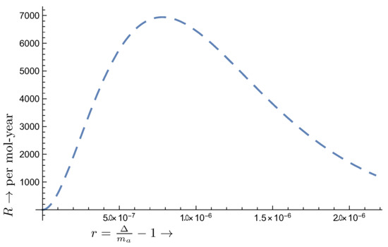
Figure 7.
The only possible transition is of A type. Now the transition energy is eV. The extracted axion mass is given by the value of at the location of the maximum, , analogous to that of Equation (47). The width is determined by , where and are the locations at half maximum.
(ii) p-orbitals.
The event rate is exhibited in Figure 8.
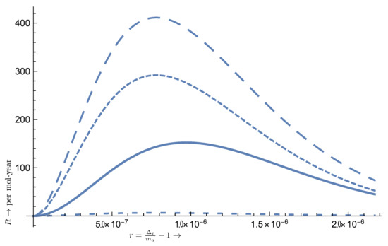
Figure 8.
The rate as a function of , for transition types indicated by a long dash, short dash, solid line, and intermediate dash, respectively. Note that to make the type A fit in the picture, we have suppressed it by the factor , i.e., its actual value is 5 times larger. In these plots, the shape is essentially determined by the velocity distribution. The extraction of the axion mass and the width of the resonance are determined as in Figure 7, except that mow , and , . The obtained results for the axion mass and the extracted width may not agree exactly with those of Equations (47) and (33), respectively, due to the fact that the resonances here are not normalized. The parameters are as follows: , , , . In the case of 13Al considered here eV. For any other single particle p-orbitals only may be different.
(iii) d-orbitals.
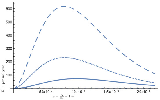
Figure 9.
The same as in Figure 8 in the case of the atom 21Sc. The parameters are as follows: , , , , with eV.
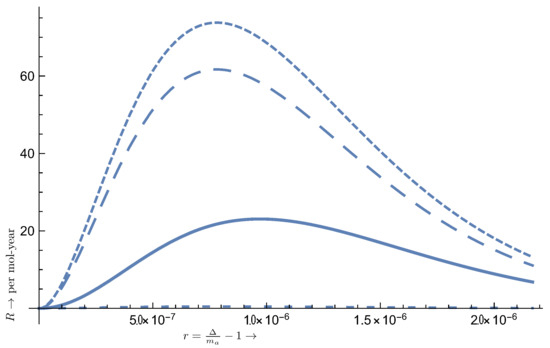
Figure 10.
The same as in Figure 9 in the case of the atom 39Y, which also involves d-orbitals, but in this case eV. For transition type A, the suppression factor was employed, i.e., the corresponding rate must be multiplied by 10.
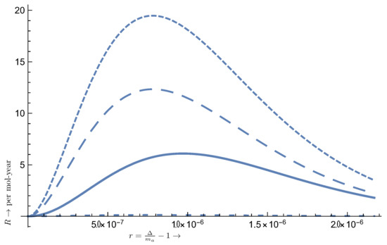
Figure 11.
The same as in Figure 9 in the case of the atom 71Lu, which also involves d-orbitals, but in this case eV. Again, for transition type A, the suppression factor was employed.
7.2. Two-Electron Configurations
In this case we will consider the two systems discussed in Section 5.2.1, namely carbon and 22Ti.
In the first case the transition is 3, i.e., since the initial initial state is a , the A type transition is not available. The obtained rates are exhibited in Figure 12. It may be useful to note that the Si atom has the same structure, except for the radial quantum number, which is irrelevant here, and the fact that eV. Otherwise, the situation is the same as in Figure 12.
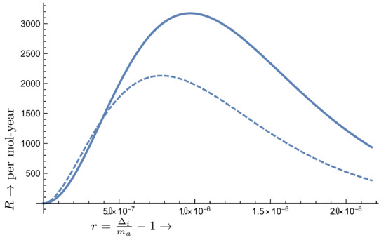
Figure 12.
The same as in Figure 8 but for the C atom, with as follows: , , , eV. The patterns B and D coincide, while the type A transition is not present.
For the second target 22Ti, the transition is 3, with the splitting of the spin-orbit partners being relatively small. The obtained results are exhibited in Figure 13. The use of such a target, however, may suffer from the fact that 22Ti normally exists in metallic form. It may be useful to note that the neutral Zr (Zr I) atom has the same structure, except for the radial quantum number, which is irrelevant here, and the fact that eV. Otherwise, the situation is the same as in Figure 13.
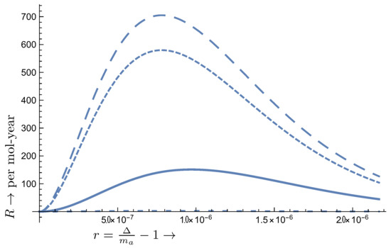
Figure 13.
The same as in Figure 8 but for the Ti atom. For transition type A, the suppression factor was employed, i.e., the corresponding rate must be multiplied by 5. Now given by , , , , eV. The The type D transition is not visible.
7.3. Many-Electron Configurations
In this case, we will consider the two targets described in Section 5.2.2.
(i) Transitions of the type 3.
The simplest such system is the oxygen atom with . As has already been mentioned, one may also consider sulfur (S I), which has the same configuration but a different n, i.e., .
(ii) The second interesting example of many particle configurations is that of 26Fe, allowing the transition 5.
The obtained results presented in Figure 14.
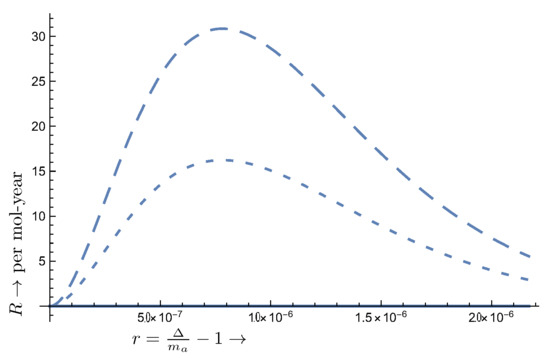
Figure 14.
The same as in Figure 8 but for the iron target. The A term has been suppressed by a factor of 1/500, i.e., its actual value is 500 times larger. Now with , , eV. The other two transition types do not occur.
At this point, we should mention that, for the configurations with more than a single electron, some of the rates are enhanced due to the large spin interaction involved, see Table 2.
7.4. A Summary of the Obtained Results
We have exhibited the results for the axion-induced excitations for a number of atomic targets; see Figure 7, Figure 8, Figure 9, Figure 10, Figure 11, Figure 12, Figure 13, Figure 14 and Figure 15. Similar results are expected for targets involving different radial functions with the same angular momentum structure, e.g., single-particle structures involving s, p, and d orbitals or many-particle configurations, Si instead of C, Zr instead of Ti, etc. The expected event rates, the width of the resonance, and the dependence on the magnetic field will be the same. Only the extracted value of the axion mass from the B, C, and D terms will be different since it depends on the experimentally determined spin-orbit splitting .
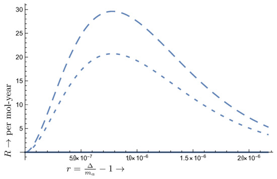
Figure 15.
The same as in Figure 8 but for the oxygen target. The A term has been suppressed by a factor of 1/500, i.e., its actual value is 500 times larger. Now with , , eV. The other two transition types do not occur. The other two transition types do not occur.
We have seen that in all atoms considered, the expected resonances are very narrow, and since we have no experimental or theoretical information about the axion mass, they might be missed by experiments. The location of the resonance, however, depends on the magnetic field employed. One, thus, may consider a magnetic field whose magnitude is changing periodically from a minimum to a maximum value many times during the experiment. The oscillation period must be as short as possible and, in any case, very much shorter than the run time of the experiment. The duration of the run must be longer than the time implied by the predicted event rate to compensate for the fact that only a fraction of the time, the equipment is going to be at the right state of sensitivity for axion detection. With this arrangement, one can perhaps see the axion provided its mass lies between and for . This range depends on the atom considered. The most favored case is the one with as large as possible magnetic moment splitting. Thus in the case of the iron target, one can detect light axion masses through the A term in the range of , with n an integer. In particular for n = 100 and T one can detect axions in the mass range . This range is a bit wider than that of the dedicated experiments involving resonant cavities, such as the well-known ADMX, ADMX-HF, and CAP [22], searching for axion masses, see, e.g., [15,17,20]. For a summary, see [27] and a recent review [48] giving the range (values eV have recently been excluded by ADMX [30]).
Similarly, for heavier axions through the D term, one obtains a relation depending on the spin-orbit splitting, in this case, .
The width of the above window can, of course, increase if larger magnetic fields are employed, consistent, of course, with the constraints discussed in Section 6, and the minimum can be selected to be the convenient one. We should add that, after consultation of our diagram of Figure 6 and Table 3, we obtain for an axion mass of 1 meV a required temperature between 1.5 and 5 Kelvin. This temperature range is almost identical to the one investigated experimentally by Braggio et al. [46], with the final verdict being that efficient heat dissipation for such conditions is quite feasible. Thus, there are no laser heating problems for the 1 meV to 1 eV range. We recognize that, for the meV range, it would be certainly more challenging. Given, however, the numerous studies on cold atoms where temperatures of the order of hundreds of Kelvins are achieved (admittedly for small samples) we believe it would be still feasible to achieve at least 0.1 Kelvin, even when dealing with large samples (axion masses around eV, see our Figure 6).
Table 3.
The maximum in Kelvin temperature acceptable as a function of the axion mass for the condition that the Boltzmann factor given by Equation (43) must be less than
Anyway, such windows of axion mass can be open in atomic physics detection, provided that the sweep in frequency is smooth and gap-less, exploiting the feasibility of a simultaneous scan of the frequency of the exciting radiation (presumably delivered by a laser) for the transition of as suggested by Sikivie and that of the magnetic field in a prescribed way (see, e.g., [49,50]).
This way one would think that the narrowness of the signal is beneficial rather than problematic, yielding an advantage of the atomic experiments against the background.
8. Conclusions
In this paper, we considered the possibility of direct detection of axion as a dark matter candidate by measuring the rates for axion-induced atomic excitations. The essential input in our calculations was the strength of the axion electron interaction and the axion flux on the detector. For the latter, we have used the standard halo parameters with a Maxwell–Boltzmann distribution transformed in the local frame. The strength of the interaction was assumed to be equal to the limit obtained from the Borexino experiment. This assumption allows axion masses in the range that can be exploited by spin-induced atomic transitions. That is tens of eV within members of the same multiplet, i.e., of the type A, and axion masses in the range 1 meV–1 eV involving transitions of to the type (types of B, C and D) allowed by the angular momentum selection rules.
Furthermore, since the axion is absorbed by the atom, the calculated cross-section exhibits resonant behavior. The resulting pattern reflects the parameters of the velocity distribution in the local frame and the momentum dependence of the axion-electron interaction. The obtained results depend, of course, on the atom considered through the parameters (the spin-orbit splitting) and (the energy splitting due to the magnetic moment interaction). These two parameters determine the axion mass that can be detected, which is very close to the excitation energy. In addition the resonant behavior can be exploited by experiments in minimizing any background events.
In the special case of the type A transitions the obtained rates, as shown at the top of the resonance, are quite large as a result of the large axion flux. The highest rates obtained occur in the case of light axions. They involve all the transitions in any atom and the A type transitions and for the many-electron configuration atoms like Oxygen and 28Fe, namely and per mole-y, respectively. The experimental detection difficulty, in this case, is not connected with the expected rate but, as explained in Section 6, with the cryogenic temperature behavior of the target. The excited state must be essentially empty of electrons. For the A-term, the largest mass that can be detected is 185 eV. The highest temperature in Kelvin that can be tolerated depends on x, and is shown in Table 3. Furthermore, the target must exhibit atomic behavior at such cryogenic temperatures. It may be an advantage that such high rates allow one to consider the atom of interest in the form of an impurity at the level or even in an otherwise inert target.
For the B, C, and D type transitions the temperature requirements are not very stringent. The expected rates, as appearing at the tops of some of the B, C, D patterns in the figures, are much smaller than those of the A terms, see Figure 8, Figure 9, Figure 10, Figure 11, Figure 12, Figure 13 and Figure 14, but perhaps detectable. In the case of the 22Ti a rate as high as per mole-y is obtained.
As we have mentioned in the introduction, the axion-electron coupling can be extracted from astrophysical observations, e.g., from recent astrophysical data [35,36,37]. These experiments do not extract this coupling directly, but, with the aid of suitable axion models, they determine it from a selection among processes like the Primakoff effect shown in Figure 1b, photon conversion into an axion in the electric field of electrons or ions in the plasma:
as well as Compton scattering:
These authors present their results in terms of a dimensionless coupling constant (we intentionally use the capital letter A to avoid confusion with employed in the present work). The obtained limits are: [35], [36] and [37]. Transforming these to the units employed in this work, via the relation with the mass of the electron in GeV, we obtain , and , respectively. These must be compared with the value given by Equation (28) employed here, which has been obtained from direct experiments.
We should mention that the obtained rates vary quadratically with the elementary axion-electron coupling. This affects both the light and the heavier axions. Thus, proceeding as above for the discussion for impurity target, if the impurity is not too small, in the case of light axions, we can tolerate a coupling about 100 times smaller. In the case of the heavy axions, however, even with favorable targets like 22Ti, we estimate that the coupling should not be more than an order of magnitude smaller for such axions to be detectable. This is really an experimental problem since it depends on some factors like the size of the target.
The main experimental problem for all types of transitions is due to the fact that all resonances are very narrow and they might be missed by the experiments. This is, unfortunately, so since there is no experimental or theoretical guide about the expected value of the axion mass. We have seen, however, that if a suitable periodic magnetic field is selected, whose magnitude is in an appropriate range and its period is very much smaller than the experimental run time, a window of axion mass in the range of a fraction of an meV wide, becomes open, which may be adequate.
Author Contributions
Conceptualization, methodology, formal analysis, J.D.V.; validation, review and editing, S.C.; validation, F.T.A.; visualization, R.C. All authors have read and agreed to the published version of the manuscript.
Funding
This research received no external funding.
Data Availability Statement
We agree to share our research data and datasets analyzed or generated during the study.
Acknowledgments
Special thanks to Yannis Semertzidis, director of the Center for Axion and Precision Physics Research, IBS, at KAIST University, for his hospitality, encouragement and useful discussions. All authors are indebted to Pierre Sikivie for a careful reading of the manuscript and his very useful comments and suggestions, as well as bringing to their attention the need for a simultaneous scan of frequency and magnetic field. Special thanks to Hiroyasu Ejiri for clarifying some aspects of the experiment proposed in this work.
Conflicts of Interest
The authors declare no conflicts of interest.
Appendix A. The Modulation of the Widths
The modulation of the widths can be simply included by making the local frame the replacement:
where is the phase of the Earth, around June 3rd, and the ratio of Earth’s velocity around the sun divided by the sun’s velocity around the galaxy, . We thus obtain a time variation of the width shown in Figure A1. We see that the effect is small, the difference between the maximum and the minimum is less than , almost the same with that obtained in the axion to photon conversion [44]. We note, however, that, in addition to the seasonal dependence, we have a dependence on the magnetic quantum numbers of the states involved. The variation in the case of is almost twice as large compared to that with .
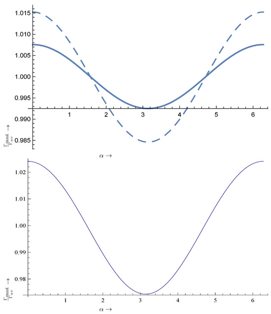
Figure A1.
In the top panel we exhibit the modulation of the width , relative to its average value, as a function of the phase of the Earth. The solid line corresponds to the case (no change in the magnetic quantum number) while the dashed one corresponds . For comparison, we present in the bottom panel the modulation curve obtained in the case of the standard axion to photon conversion, obtained with the same halo parameters [44].
It is amusing to know that the dispersion also exhibits a time dependence (see Figure A2).
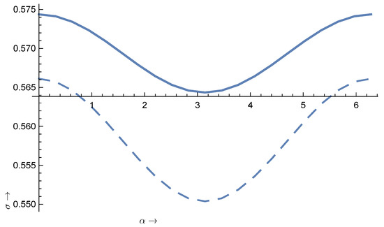
Figure A2.
The time variation of the width for axion absorption by an atom due to the motion of the Earth. The notation for the curves is the same as in Figure A1.
References
- Peccei, R.; Quinn, H. CP Conservation in the Presence of Pseudoparticles. Phys. Rev. Lett. 1977, 38, 1440. [Google Scholar] [CrossRef]
- Weinberg, S. A New Light Boson? Phys. Rev. Lett. 1978, 40, 223. [Google Scholar] [CrossRef]
- Wilczek, F. Problem of Strong P and T Invariance in the Presence of Instantons. Phys. Rev. Lett. 1978, 40, 279. [Google Scholar] [CrossRef]
- Kim, J.E. Weak-Interaction Singlet and Strong CP Invariance. Phys. Rev. Lett. 1979, 43, 137. [Google Scholar] [CrossRef]
- Shifman, M.A.; Vainshtein, A.; Zakharov, V.I. Can Confinement Ensure Natural CP Invariance of Strong Interactions? Nucl. Phys. B 1980, 166, 493. [Google Scholar] [CrossRef]
- Dine, M.; Fischler, W.; Srednicki, M. A simple solution to the strong CP problem with a harmless axion. Phys. Lett. B 1981, 104, 199. [Google Scholar] [CrossRef]
- Zhitnisky, A. On Possible Suppression of the Axion Hadron Interactions. Sov. J. Nucl. Phys. 1980, 31, 260. (In Russian) [Google Scholar]
- Abbott, L.F.; Sikivie, P. A cosmological bound on the invisible axion. Phys. Lett. B 1983, 120, 133. [Google Scholar] [CrossRef]
- Dine, M.; Fischler, W. The not-so-harmless axion. Phys. Lett. 1983, 120, 137. [Google Scholar] [CrossRef]
- Preskill, J.; Wise, M.B.; Wilczek, F. Cosmology of the invisible axion. Phys. Lett. 1983, 120, 127. [Google Scholar] [CrossRef]
- Asztalos, S.J.; Carosi, G.; Hagmann, C.; Kinion, D.; Van Bibber, K.; Hotz, M.; Rosenberg, L.J.; Rybka, G.; Hoskins, J.; Hwang, J.; et al. SQUID-based microwave cavity search for dark-matter axions. Phys. Rev. Lett. 2010, 104, 041391. [Google Scholar] [CrossRef]
- Duffy, L.; Sikivie, P.; Tanner, D.B.; Asztalos, S.; Hagmann, C.; Kinion, D.; Rosenberg, L.J.; van Bibber, K.; Yu, D.; Bradley, R.F. Results of a Search for Cold Flows of Dark Matter Axions. Phys. Rev. Lett. 2005, 95, 091304. [Google Scholar] [CrossRef]
- Wagner, A.; Rybka, G.; Hotz, M.; Rosenberg, L.J.; Asztalos, S.J.; Carosi, G.; Hagmann, C.; Kinion, D.; Van Bibber, K.; Hoskins, J.; et al. Search for hidden sector photons with the ADMX detector. Phys. Rev. Lett. 2010, 105, 171801. [Google Scholar] [CrossRef]
- Irastorza, I.G.; García, J.A. Direct detection of dark matter axions with directional sensitivity. J. Cosmol. Astropart. Phys. 2012, 1210, 22. [Google Scholar] [CrossRef]
- Shokair, T.M.; Root, J.; Van Bibber, K.A.; Brubaker, B.; Gurevich, Y.V.; Cahn, S.B.; Lamoreaux, S.K.; Anil, M.A.; Lehnert, K.W.; Mitchell, B.K.; et al. Future directions in the microwave cavity search for dark matter axions. Int. J. Mod. Phys. A 2014, 29, 1443004. [Google Scholar] [CrossRef]
- Sikivie, P. Experimental tests of the invisible axion. Phys. Rev. Lett. 1983, 51, 1415. [Google Scholar] [CrossRef]
- Primack, J.; Seckel, D.; Sadoulet, B. Detection of Cosmic Dark Matter. Annu. Rev. Nucl. Part. Sci. 1988, 38, 751. [Google Scholar] [CrossRef]
- Arik, M.; Aune, S.; Barth, K.; Belov, A.; Borghi, S.; Bräuninger, H.; Cantatore, G.; Carmona, J.M.; Cetin, S.A.; Collar, J.I.; et al. Search for Sub-eV Mass Solar Axions by the CERN Axion Solar Telescope with 3He Buffer Gas. Phys. Rev. Lett. 2011, 107, 261302. [Google Scholar] [CrossRef] [PubMed]
- Arvanitaki, A.; Dimopoulos, S.; Dubovsky, S.; Kaloper, N.; March-Russell, J. String axiverse. Phys. Rev. D 2010, 81, 123530. [Google Scholar] [CrossRef]
- Stern, I.P. ADMX and collaborations. Axion dark matter searches. AIP Conf. Proc. 2014, 1604, 456–461. [Google Scholar]
- Rybka, G. The Axion Dark Matter Experiment, IBS MultiDark Joint Focus Program WIMPs and Axions; IBS Center for Theoretical Physics of the Universe (CTPU): Daejeon, Republic of Korea, 2014. [Google Scholar]
- Center for Axion and Precision Physics Research (CAPP), Daejeon 305–701, Republic of Korea. Available online: https://capp.ibs.re.kr/html/capp_en/ (accessed on 19 January 2024).
- Asztalos, S.J.; Carosi, G.; Hagmann, C.; Kinion, D.; Van Bibber, K.; Hotz, M.; Rosenberg, L.J.; Rybka, G.; Wagner, A.; Hoskins, J.; et al. Design and performance of the ADMX SQUID-based microwave receiver. Nucl. Instrum. Methods Phys. Res. Sect. A Accel. Spectrometers Detect. Assoc. Equip. 2011, A656, 39. [Google Scholar] [CrossRef]
- Lee, S.; Ahn, S.; Choi, J.; Ko, B.R.; Semertzidis, Y.K. Axion dark matter search around 6.7 μeV. Phys. Rev. Lett. 2020, 124, 101802. [Google Scholar] [CrossRef]
- Kim, D.; Jeong, J.; Youn, S.; Kim, Y.; Semertzidis, Y.K. Revisiting the detection rate for axion haloscopes. J. Cosmol. Astropart. Phys. 2020, 3, 66. [Google Scholar] [CrossRef]
- Semertzidis, Y.K.; Kim, J.E.; Youn, S.; Choi, J.; Chung, W.; Haciomeroglu, S.; Kim, D.; Kim, J.; Ko, B.; Kwon, O.; et al. Axion dark matter research with IBS/CAPP. arXiv 2019, arXiv:1910.11591. [Google Scholar]
- Raffelt, G. Astrophysical Axion Bounds, IBS MultiDark Joint Focus Program WIMPs and Axions; Institute for Basic Science: Daejeon, Republic of Korea, 2014. [Google Scholar]
- Du, N.; Force, N.; Khatiwada, R.; Lentz, E.; Ottens, R.; Rosenberg, L.J.; Rybka, G.; Carosi, G.; Woollett, N.; Bowring, D.; et al. Search for invisible axion dark matter with the axion dark matter experiment. Phys. Rev. Lett. 2018, 120, 151301. [Google Scholar] [CrossRef]
- Brain, T.; Cervantes, R.; Crisosto, N.; Du, N.; Kimes, S.; Rosenberg, L.J.; Rybka, G.; Yang, J.; Bowring, D.; Chou, A.S.; et al. Extended Search for the Invisible Axion with the Axion Dark Matter Experiment. Phys. Rev. Lett. 2020, 124, 101303. [Google Scholar] [CrossRef] [PubMed]
- Bartram, C.; Braine, T.; Burns, E.; Cervantes, R.; Crisosto, N.; Du, N.; Korandla, H.; Leum, G.; Mohapatra, P.; Nitta, T.; et al. Search for Invisible Axion Dark Matter in the 3.3–4.2 μeV Mass Range. Phys. Rev. Lett. 2021, 127, 261803. [Google Scholar] [CrossRef]
- Zioutas, K.; Semertzidis, Y. A new detector scheme for axions. Phys. Lett. A 1988, 130, 94. [Google Scholar] [CrossRef]
- Tan, H.T.; Flambaum, V.V.; Samsonov, I.B.; Stadnik, Y.V.; Budker, D. Interference-assisted resonant detection of axions. Phys. Dark Universe 2019, 24, 100272. [Google Scholar]
- Flambaum, V.V.; Samsonov, I.B.; Tan, H.B.T.; Budker, D. Coherent axion-photon transformations in the forward scattering on atoms. arXiv 2018, arXiv:1805.01793. [Google Scholar] [CrossRef]
- Sikivie, P. Axion dark matter detection using atomic transitions. Phys. Rev. Lett. 2014, 113, 201301. [Google Scholar] [CrossRef]
- Fu, C.; Zhou, X.; Chen, X.; Chen, Y.; Cui, X.; Fang, D.; Giboni, K.; Giuliani, F.; Han, K.; Huang, X.; et al. Limits on axion couplings from the first 80 days of data of the pandax-ii experiment. Phys. Rev. Lett. 2017, 119, 181806. [Google Scholar] [CrossRef]
- Straniero, O.; Pallanca, C.; Dalessandro, E.; Dominguez, I.; Ferraro, F.R.; Giannotti, M.; Mirizzi, A.; Piersanti, L. The RGB tip of galactic globular clusters and the revision of the axion-electron coupling bound. Astronomy Astrophys. 2020, 644, A106. [Google Scholar] [CrossRef]
- Luzio, L.D.; Fedele, M.; Giannotti, M.; Mescia, F.; Nardi, E. Stellar evolution confronts axion models. J. Cosmol. Astropart. Phys. 2022, 2, 35. [Google Scholar] [CrossRef]
- Bellini, G.; Benziger, J.; Bick, D.; Bonfini, G.; Bravo, D.; Avanzini, M.B.; Caccianiga, B.; Cadonati, L.; Calaprice, F.; Carraro, C.; et al. Search for solar axions produced in the p (d, 3He)A reaction with Borexino detector. Phys. Rev. D 2012, 85, 092003. [Google Scholar] [CrossRef]
- Vergados, J.D. Searching for light WIMPs via their interaction with electrons. J. Phys. G 2020, 47, 095007. [Google Scholar] [CrossRef]
- Gorghetto, M.; Villadoro, G. Topological susceptibility and QCD axion mass: QED and NNLO corrections. J. High Energy Phys. 2019, 2019, 33. [Google Scholar] [CrossRef]
- Vergados, J.D.; Divari, P.C.; Ejiri, H. Calculated Event Rates for Axion Detection via Atomic and Nuclear Processes. Adv. High Energy Phys. 2022, 2022, 7373365. [Google Scholar] [CrossRef]
- Di Cortona, G.G.; Hardy, E.; Vega, J.P.; Villadoro, G. The QCD axion, precisely. J. High Energy Phys. 2016, 1, 34. [Google Scholar] [CrossRef]
- Ringwald, A.; Saikawa, K.I. Axion dark matter in the post-inflationary Peccei-Quinn symmetry breaking scenario. Phys. Rev. D 2016, 93, 085031. [Google Scholar] [CrossRef]
- Vergados, J.D.; Semertzidis, Y.K. Axionic dark matter signatures in various halo models. Nucl. Phys. B 2017, 915, 10. [Google Scholar] [CrossRef]
- Vergados, J.D. Group and Reprsentaion Theory; World Scientific: Singapore, 2017. [Google Scholar]
- Braggio, C.; Carugno, G.; Chiossi, F.; Lieto, A.D.; Guarise, M.; Maddaloni, P.; Ortolan, A.; Ruoso, G.; Santamaria, L.; Tasseva, J.; et al. Axion dark matter detection by laser induced fluorescence in rare-earth doped materials. Sci. Rep. 2017, 7, 15168. [Google Scholar] [CrossRef] [PubMed]
- Doherty, M.W.; Manson, N.B.; Delaney, P.; Jelezko, F.; Wrachtrup, J.; Hollenberg, L.C. The nitrogen-vacancy colour centre in diamond. Phys. Rep. 2013, 528, 1. [Google Scholar] [CrossRef]
- Ringwald, A. Alternative dark matter candidates: Axions. arXiv 2016, arXiv:1612.08933. [Google Scholar]
- Delande, D.; Taylor, K.; Haley, M.; van der Veldt, T.; Vassen, W.; Hogervorst, W. Scaled energy spectra of non-hydrogenic Rydberg atoms in a magnetic field. J. Phys. B At. Mol. Opt. Phys. 1994, 27, 2771. [Google Scholar] [CrossRef]
- Leach, R. Fundamental Principles of Engineering Nanometrology; Elsevier: Amsterdam, The Netherlands, 2014. [Google Scholar]
Disclaimer/Publisher’s Note: The statements, opinions and data contained in all publications are solely those of the individual author(s) and contributor(s) and not of MDPI and/or the editor(s). MDPI and/or the editor(s) disclaim responsibility for any injury to people or property resulting from any ideas, methods, instructions or products referred to in the content. |
© 2024 by the authors. Licensee MDPI, Basel, Switzerland. This article is an open access article distributed under the terms and conditions of the Creative Commons Attribution (CC BY) license (https://creativecommons.org/licenses/by/4.0/).