Control-Oriented Free-Boundary Equilibrium Solver for Tokamaks

Abstract

A free-boundary equilibrium solver for an axisymmetric tokamak geometry was developed based on the finite difference method and Picard iteration in a rectangular computational area. The solver can run either in forward mode, where external coil currents are prescribed until the converged magnetic flux function $\psi (R,Z)$ map is achieved, or in inverse mode, where the desired plasma boundary, with or without an X-point, is prescribed to determine the required coil currents. The equilibrium solutions are made consistent with prescribed plasma parameters, such as the total plasma current, poloidal beta, or safety factor at a specified flux surface. To verify the mathematical correctness and accuracy of the solver, the solution obtained using this numerical solver was compared with that from an analytic fixed-boundary equilibrium solver based on the EAST geometry. Additionally, the proposed solver was benchmarked against another numerical solver based on the finite-element and Newton-iteration methods in a triangular-based mesh. Finally, the proposed solver was compared with equilibrium reconstruction results in DIII-D experiments.

1. Introduction

Plasma equilibrium is a fundamental state in magnetic confinement fusion devices, such as stellarators and tokamaks. Plasma equilibrium models, which are based on the force balance equation, are frequently used to explore various aspects of plasma operations. These models are essential for determining optimal plasma shapes; studying physics issues such as magnetohydrodynamic (MHD) instabilities, turbulence, and transport; and assessing nominal plasma scenarios.

Plasma equilibrium problems in an axisymmetric tokamak geometry can be broadly classified into two categories. One is the fixed-boundary equilibrium (FXBE) problem, where the plasma boundary is prescribed, and only the internal distributions of plasma profiles are of interest. The fixed-boundary equilibrium assumption is widely adopted in MHD and transport analysis because this equilibrium problem can be solved quickly, both analytically and numerically. The other type is the free-boundary equilibrium (FBE) problem, where the plasma boundary is unknown and is identified by the resulting poloidal magnetic flux distribution. This distribution is determined by the external coil currents and the current flowing toroidally within the plasma. The FBE problem is widely used to design plasma shape control strategies and to reconstruct plasma equilibrium profiles using diagnostic measurements in tokamak experiments.

Many equilibrium solvers that address the FXBE problem rely on analytical approaches with simplified assumptions, though there are also numerical solvers, such as TEQ [1], that handle the FXBE problem in a more complex manner. The typical analytic FXBE solvers, using a linear or constant distribution of plasma current density, are based on an up–down symmetric plasma boundary prescribed by either four points [2] or parameters with X-points [3]. Recently, a more general fixed-boundary equilibrium solver [4] was proposed. It is compatible with both vertically symmetric and asymmetric plasma boundaries and uses a smoothed and monotonic plasma profile, i.e., the toroidal plasma current density. However, to accurately consider realistic plasma dynamics with respect to poloidal field (PF) systems in tokamaks, especially for magnetic control, developing an FBE solver where external coils serve as actuators is of high priority. Unlike FXBE solvers, solvers for the FBE problem can only be tackled numerically in an iterative manner due to the nonlinearity of the plasma current density. There are two dominant approaches in the literature for addressing the FBE problem on different computational grids. One approach is based on the finite element method (FEM) and Newton-type iteration on a triangular-based grid, as seen in the codes for the C++ version of CEDRES++ [5] and the MATLAB version of FEEQS.M [6], which have been used to design plasma operational scenarios for WEST [7] and ITER [8]. These FEM-based FBE solvers can find numerical solutions with high accuracy (iterative error less than ${10}^{-10}$) and handle nonlinear issues, such as iron permeability. In tokamaks, like JET [9] and WEST, areas with nonlinear magnetic permeability, such as those containing iron, are used to extend the pulse length. However, this introduces additional complexity for the solver to address. Moreover, the large and complicated computational mesh usually makes them computationally intensive. The other approach is performed on a simple and small-sized rectangular grid and is solved by Picard iteration, e.g., the TSC [10] and TES [11] codes. These simplified mesh constructions and fast computations make them more attractive, especially for fast integrated scenario predictions.

In this work, a numerical FBE solver named the Control-Oriented Tokamak Equilibrium Solver (COTES) is introduced. It is based on the finite difference method (FDM) and operates fully within MATLAB/SIMULINK©, which is considered the standard platform for control design. Unlike previous approaches [11,12], COTES employs a sophisticated vertical shift of the plasma current density to address the numerical issues, e.g., vertical instability problem, during iterations in asymmetric plasma shapes, rather than adding fictitious coil currents to feedback vertical excursions. Various dedicated numerical simulations were conducted through COTES for superconducting (EAST) and conventional (DIII-D) tokamak geometries. These simulations were cross-checked with a fixed-boundary solver and the finite-element and Newton-iteration FEEQS.M solver to address benchmarks between different FBE solvers that were seldom undertaken in previous studies. Dedicated COTES simulations were also conducted to verify different approaches for the control of vertical instability based on experimental equilibrium reconstruction data with the EFIT code [13].

This paper is organized as follows. In Section 2, the FBE equations and the numerical approach used in COTES are introduced in detail. Section 3 covers the benchmarks and verifications, including the mathematical accuracy and correctness against a fixed-boundary solution, numerical comparisons with FEEQS.M, and experimental reconstruction data. Finally, conclusions and possible future work are presented in Section 4.

2. Numerical Approach in COTES

The main FBE equation and approach implemented in COTES follow the previous works of [11,12]. This section emphasizes the new treatments developed in COTES and the details that were missed in previous approaches.

2.1. Free-Boundary Equilibrium Problem in Tokamak Geometry

In the cylindrical coordinate system ($R,\varphi ,Z$), the $\varphi$ component is considered negligible due to the assumption of toroidal axisymmetry in tokamaks. The FBE equation, derived from the force balance equation for an air-core tokamak, is written as follows:

$$\begin{array}{cc}\hfill {\mathsf{\Delta }}^{*}\psi (R,Z)& =-{\mu }_{0}R{J}_{\varphi }(R,Z),\end{array}$$

(1a)

$$\begin{array}{cc}\hfill {\mathsf{\Delta }}^{*}& \equiv R{\displaystyle \frac{\partial }{\partial R}}\left({\displaystyle \frac{1}{R}}{\displaystyle \frac{\partial }{\partial R}}\right)+{\displaystyle \frac{{\partial }^2}{\partial Z^2}},\end{array}$$

(1b)

where the poloidal flux function $\psi$, known as the poloidal magnetic flux per radian, is defined as $\psi (R,Z)\equiv R{A}_{\varphi }$ from $B=\nabla \times \mathbf{A}$, and ${\mu }_0$ is the permeability in a vacuum. The right-hand side (RHS) of Equation (1a) is the toroidal current density, which is dependent on different factors:

$$\begin{array}{c}\hfill J_{\varphi }(R,Z)=\left\{\begin{array}{cc}R{p}^{\prime }\left(\psi \right)+{\displaystyle \frac{f{f}^{\prime }\left(\psi \right)}{{\mu }_{0}R}}\hfill & \mathrm{in}\mathrm{plasma}\mathrm{area}{\mathsf{\Omega }}_{pl}\hfill \\ {\displaystyle \frac{I_c}{S_c}}\hfill & \mathrm{in}\mathrm{coil}\mathrm{number}c\hfill \\ 0\hfill & \mathrm{elsewhere},\hfill \end{array}\right.\end{array}$$

(2)

in which p represents the plasma kinetic pressure, f is the diamagnetic function defined as $f\left(\psi \right)\equiv R{B}_{\varphi }$, $B_{\varphi }$ is the toroidal magnetic field, $I_c$ and $S_c$ are the current and cross-section of the external conductor coil c, and the prime sign represents the derivative with regard to $\psi$. The toroidal plasma current density, $J_{\varphi ,pl}(R,Z)$, is derived from the well-known Grad–Shafranov (G-S) equation [14,15]. It is important to note that currents on possible passive plates and vacuum vessel, induced by plasma vertical excursions and disruptions, can also be treated as having similar current densities to those in the external coils. These induced currents are very important to reduce the growth rate of plasma vertical events (VDEs) due to a loss of control in the vertical position, disruption, and MHD instabilities [16].

The $J_{\varphi ,pl}(R,Z)$ is parameterized from [17] as

$$\begin{array}{c}\hfill J_{\varphi ,pl}(R,Z)=\lambda \left[{\beta }_0{\displaystyle \frac{R}{R_0}}{(1-{\psi }_N^{{\alpha }_m})}^{{\alpha }_n}+(1-{\beta }_0){\displaystyle \frac{R_0}{R}}{(1-{\psi }_N^{{\beta }_m})}^{{\beta }_n}\right],\end{array}$$

(3a)

$$\begin{array}{c}\hfill p^{\prime }\left(\psi \right)\equiv {\displaystyle \frac{\lambda {\beta }_0}{R_0}}{(1-{\psi }_N^{{\alpha }_m})}^{{\alpha }_n},f{f}^{\prime }\left(\psi \right)\equiv \lambda {\mu }_0{R}_0(1-{\beta }_0){(1-{\psi }_N^{{\beta }_m})}^{{\beta }_n},\end{array}$$

(3b)

where $R_0$ is the major radius, and ${\psi }_N\in [0,1]$ is the normalized $\psi$ defined as ${\psi }_N\equiv (\psi -{\psi }_{ax})/({\psi }_{bd}-{\psi }_{ax})$, where ${\psi }_{ax}$ and ${\psi }_{bd}$ are the $\psi$ along the plasma axis and at the boundary, respectively. The parameters $\lambda$ and ${\beta }_0$ can be tuned to constrain the specified equilibrium, which are discussed further below, while ${\alpha }_m,{\alpha }_n,{\beta }_m$, and ${\beta }_n$ are user-defined input constants.

When solving the FBE equation through numerical methods, certain plasma quantities can be prescribed. Two unknowns, i.e., $\lambda$ and ${\beta }_0$ in Equation (3), can be determined to satisfy two constrained parameters. These parameters could be imposed on plasma quantities, such as $I_p$ and the poloidal plasma beta (${\beta }_p$):

$$\begin{array}{cc}\hfill I_p& ={\int }_{{\mathsf{\Omega }}_{pl}}{J}_{\varphi ,pl}(\lambda ,{\beta }_0)d\mathsf{\Omega },\end{array}$$

(4a)

$$\begin{array}{cc}\hfill {\beta }_p& =2{\mu }_0{\displaystyle \frac{⟨p(\lambda ,{\beta }_0)⟩}{⟨B_p^2⟩}},\end{array}$$

(4b)

where $B_p={\displaystyle \frac{1}{R}}\nabla \psi \times {\widehat{e}}_{\varphi }$ (toroidal unit vector) is the poloidal magnetic field. The bracket $⟨·⟩$ denotes the flux-averaging operation [18] for arbitrary term A with

$$\begin{array}{c}\hfill ⟨A⟩={\displaystyle \frac{\partial }{\partial V}}{\int }_{V}AdV={\displaystyle \frac{{\int }_{D}AdV}{{\int }_{D}dV}}={\displaystyle \frac{{\int }_{\mathsf{\Omega }pl}ARdS}{{\int }_{{\mathsf{\Omega }}_{pl}}RdS}}\end{array}$$

(5a)

$$\begin{array}{c}\hfill \mathrm{or}⟨A⟩={\displaystyle \frac{{\int }_{{\psi }_N}\frac{A}{B_p}dl}{{\int }_{{\psi }_N}\frac{1}{B_p}dl}},\end{array}$$

(5b)

in which D and V are the 3D plasma area and the volume inside a specified $\psi$ surface, and l is a closed flux contour.

Additionally, these two plasma parameters can also be $I_p$ and $q\left({\psi }_N\right)$ (safety factor) at a specified ${\psi }_N$, such as $q_{95}$ at ${\psi }_N=0.95$. The safety factor q is defined by

$$\begin{array}{cc}\hfill q\left({\psi }_N\right)& ={\displaystyle \frac{1}{2\pi }}{\int }_{{\psi }_N}{\displaystyle \frac{B_{\varphi }}{R{B}_p}}dl={\displaystyle \frac{1}{2\pi }}{\int }_{{\psi }_N}{\displaystyle \frac{f(\lambda ,{\beta }_0)}{R^2{B}_p}}dl,\end{array}$$

(6)

in which $f=R{B}_{\varphi }$ is used.

The continuous flux-averaged plasma quantities above can be estimated by discrete approximates, e.g., $I_p$ (similarly for ${\beta }_p$) in the plasma area based on Equations (3) and (4) or (6) as

$$\begin{array}{cc}\hfill I_p& =\lambda {\beta }_0·\left(\sum _{m=1}^{Nod{e}_{pl}}{\displaystyle \frac{R_m}{R_0}}{(1-{\psi }_{N,m}^{{\alpha }_m})}^{{\alpha }_n}\right)·\delta R\delta Z,\hfill \\ \hfill & +\lambda (1-{\beta }_0)·\left(\sum _{m=1}^{Nod{e}_{pl}}{\displaystyle \frac{R_0}{R_m}}{(1-{\psi }_{N,m}^{{\beta }_m})}^{{\beta }_n}\right)·\delta R\delta Z,\hfill \end{array}$$

(7)

where $Nod{e}_{pl}$ is a plasma element.

Similarly, $q\left({\psi }_N\right)$ on closed contour points ($R_k,Z_k$) can be approximated with Equation (6) as follows:

$$q\left({\psi }_N\right)={\displaystyle \frac{1}{2\pi }}f\left({\psi }_N\right)·\left(\sum _{x=1}^{k-1}{\displaystyle \frac{1}{R_x^2{B}_{p,x}^2}}·\sqrt{{(R_{x+1}-R_x)}^2+{(Z_{x+1}-Z_x)}^2}\right),$$

(8)

where $f\left({\psi }_N\right)$ on a given ${\psi }_N$ is calculated from [18] as

$$f\left({\psi }_N\right)=\sqrt{{\left(B_{\varphi ,0}{R}_0\right)}^2-2({\psi }_{bd}-{\psi }_{ax})\lambda {\mu }_0{R}_0(1-{\beta }_0)·{\int }_{{\psi }_N}^1{(1-{\psi }_N^{{\beta }_m})}^{{\beta }_n}dl}.$$

(9)

By combining Equations (7)–(9), specified $\lambda$ and ${\beta }_0$ values can be determined.

2.2. Numerical Approximations on a Rectangular Grid

The FBE Equation (1) is a 2D partial differential equation (PDE) with a nonlinear source. A typical treatment to solve this continuous PDE is to discretize the 2D operator using a 1D approximation with a known source term. A rectangular computational domain $(R_i,Z_j)$ is constructed as

$$\begin{array}{ccc}\hfill R_i& =R_{min}+\delta R\times (i-1),\delta R\hfill & \hfill =(R_{max}-R_{min})/(N_R-1),\\ \hfill Z_j& =Z_{min}+\delta Z\times (j-1),\delta Z\hfill & \hfill =(Z_{max}-Z_{min})/(N_Z-1),\end{array}$$

(10)

where $i=1,\cdots ,N_R$ and $j=1,\cdots ,N_z$ are the total number of grid points in the R and Z coordinates, respectively.

The 2D derivatives in the Shafranov operator ${\mathsf{\Delta }}^{*}$ from Equation (1b) can be approximated as

$$\begin{array}{c}\hfill {\displaystyle \frac{\partial \psi }{\partial R}}{|}_i\simeq {\displaystyle \frac{{\psi }_{i+1}-{\psi }_{i-1}}{2\delta R}},{\displaystyle \frac{\partial \psi }{\partial Z}}{|}_j\simeq {\displaystyle \frac{{\psi }_{j+1}-{\psi }_{j-1}}{2\delta Z}},\end{array}$$

(11a)

$$\begin{array}{c}\hfill {\displaystyle \frac{{\partial }^2\psi }{\partial R^2}}{|}_i\simeq {\displaystyle \frac{{\psi }_{i+1}-2{\psi }_i+{\psi }_{i-1}}{{\left(\delta R\right)}^2}},{\displaystyle \frac{{\partial }^2\psi }{\partial Z^2}}{|}_j\simeq {\displaystyle \frac{{\psi }_{j+1}-2{\psi }_j+{\psi }_{j-1}}{{\left(\delta Z\right)}^2}}.\end{array}$$

(11b)

Therefore, Equation (1) is rewritten as

$$\begin{array}{cc}\hfill {\displaystyle \frac{1}{{\left(\delta Z\right)}^2}}{\psi }_{j-1,i}& +\left({\displaystyle \frac{1}{{\left(\delta R\right)}^2}}+{\displaystyle \frac{1}{2R_i\left(\delta R\right)}}\right){\psi }_{j,i-1}-2\left({\displaystyle \frac{1}{{\left(\delta R\right)}^2}}+{\displaystyle \frac{1}{{\left(\delta Z\right)}^2}}\right){\psi }_{j,i}\hfill \\ \hfill & +\left({\displaystyle \frac{1}{{\left(\delta R\right)}^2}}-{\displaystyle \frac{1}{2R_i\left(\delta R\right)}}\right){\psi }_{j,i+1}+{\displaystyle \frac{1}{{\left(\delta Z\right)}^2}}{\psi }_{j+1,i}=-{\mu }_0{R}_i{J}_{{\varphi }_{j,i}},\hfill \end{array}$$

(12)

where ${\psi }_{j,i}$ and $J_{{\varphi }_{j,i}}$ denote $\psi (R_i,Z_j)$ and $J_{\varphi }(R_i,Z_j)$, respectively. If the RHS of $J_{{\varphi }_{j,i}}$ is known, then the equation above resembles a set of linear algebraic equations $\mathbf{Ax}=\mathbf{b}$ that can be solved using various methods [19], such as Jacobi’s Method, the Gauss–Seidel Method, and the Successive Over-Relaxation Method (SOR).

2.3. Initial Guess and Picard Iteration

In order to solve Equation (12), it is essential to pre-define the RHS of $J_{{\varphi }_{j,i}}$, which is nonlinear and depends on the solution ${\psi }_{j,i}$. This nonlinearity can only be addressed through an iterative scheme, starting from a guess of $J_{{\varphi }_{j,i}}$. A typical initial guess of $J_{{\varphi }_{j,i}}^0$ with a circular plasma current density [12] is given by

$$\begin{array}{c}\hfill J_{\varphi j,i}^0=\left\{\begin{array}{cc}{\displaystyle \frac{{\lambda }^0}{R}}\left(1-{\displaystyle \frac{A^2}{a_{init}^2}}\right)\hfill & \hfill \mathrm{if}{A}^2<a_{init}^2\\ 0\hfill & \hfill \mathrm{if}{A}^2⩾a_{init}^2,\end{array}\right.\end{array}$$

(13)

where $A^2={(R_i-R_{init})}^2+{(Z_j-Z_{init})}^2$, with $R_{init}$, $Z_{init}$, and $a_{init}$ being the user-defined plasma center coordinates and minor radius for the initial plasma current distribution. The constant ${\lambda }^0$ is adjusted to match the total plasma current. An initial guess of $J_{{\varphi }_{j,i}}^0$ with $I_p=$ 250 kA is shown in Figure 1. In practice, $J_{{\varphi }_{j,i}}$ from a converged solution is typically employed as an initial guess to expedite the iterations.

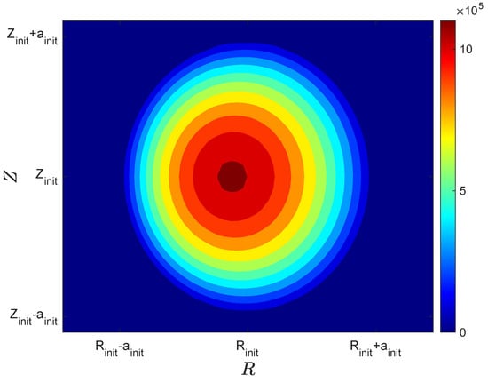
Figure 1. Initial guess of $J_{\varphi j,i}^0$ [$A/m^2$] with $I_p=$ 250 kA.

By utilizing an initial guess of $J_{{\varphi }_{j,i}}^0$, the FBE in Equation (12) can thus be solved by the well-known Picard iteration [20]. The Picard iteration is very effective for numerically solving the PDE, where the provided initial guess is close to the converged solution. The next iteration’s solution is calculated based on the current iteration in a recursive manner, which is described in detail in the following paragraph. The ${\psi }_{j,i}^n$ ($1<i<N_R,1<j<N_Z$) on the given grid, except boundary nodes, based on Equation (12) is expressed as

$$\begin{array}{cc}\hfill {\displaystyle \frac{1}{{\left(\delta Z\right)}^2}}{\psi }_{j-1,i}^n& +\left({\displaystyle \frac{1}{{\left(\delta R\right)}^2}}+{\displaystyle \frac{1}{2R_i\left(\delta R\right)}}\right){\psi }_{j,i-1}^n-2\left({\displaystyle \frac{1}{{\left(\delta R\right)}^2}}+{\displaystyle \frac{1}{{\left(\delta Z\right)}^2}}\right){\psi }_{j,i}^n\hfill \\ \hfill & +\left({\displaystyle \frac{1}{{\left(\delta R\right)}^2}}-{\displaystyle \frac{1}{2R_i\left(\delta R\right)}}\right){\psi }_{j,i+1}^n+{\displaystyle \frac{1}{{\left(\delta Z\right)}^2}}{\psi }_{j+1,i}^n=-{\mu }_0{R}_i{J}_{\varphi j,i}^n\left({\psi }_{j,i}^{n-1}\right),\hfill \end{array}$$

(14)

in which n$(n\ge 1)$ represents the n-$th$ iteration. It can be seen that $J_{{\varphi }_{j,i}}^n$, the toroidal plasma current distribution in the n-$th$ iteration, is determined by ${\psi }_{j,i}^{n-1}$, precisely specifying ${\psi }_{ax}^{n-1}$ and ${\psi }_{bd}^{n-1}$. With the assumed initial $J_{\varphi j,i}^0$, ${\psi }_{j,i}^0$ is obtained by solving Equation (14). In the next iteration, $J_{\varphi j,i}^1$ is updated based on ${\psi }_{j,i}^0$. Following this recursive iteration, the numerical solutions of $J_{\varphi j,i}^n\left({\psi }_{j,i}^{n-1}\right)$ and ${\psi }_{j,i}^n$ are obtained until a given criterion, i.e., $\parallel {\psi }_{j,i}^n-{\psi }_{j,i}^{n-1}\parallel <ϵ$ (typically ${10}^{-4}$), is satisfied. The detailed block diagram for this Picard iteration is depicted in Figure 3.

2.4. Boundary Condition for the Free-Boundary Equilibrium Solver

Equation (14) determines ${\psi }_{j,i}$ in the core region of the grid, where $1<i<N_R$ and $1<j<N_Z$. Dirichlet boundary conditions [21] are applied at the grid boundaries ($i=1,N_R$ and $j=1,N_Z$). Figure 2 illustrates the rectangular grid used to discretize the 2D computational domain $(R_i,Z_j)$ for solving the FBE Equation (1), where the spatial coordinates $R_i$ and $Z_j$ are discretized with uniform step sizes $\delta R$ and $\delta Z$, respectively. The red ’x’s mark the boundary nodes of the mesh, defining the limits of the domain, while the black dots represent the interior nodes. The boundary $\psi (R,Z)$ is computed using the Green’s function formulation [22]:

$$\psi (R,Z)=\int \int G(R,Z;R^{″},Z^{″})J_{\varphi }(R^{″},Z^{″})d{R}^{″}d{Z}^{″}/\left(2\pi \right),$$

(15)

where $G(R,Z;R^{″},Z^{″})$ is the Green’s function for a unit toroidal current source at $(R^{″},Z^{″})$, given by

$$\begin{array}{cc}\hfill G(R,Z;R^{″},Z^{″})& ={\displaystyle \frac{{\mu }_0}{2\pi }}{\displaystyle \frac{\sqrt{R{R}^{″}}}{k}}[(2-k^2)K\left(k\right)-2E\left(k\right)],\hfill \\ \hfill k^2& \equiv {\displaystyle \frac{4R{R}^{″}}{{(R+R^{″})}^2+{(Z-Z")}^2}},\hfill \end{array}$$

(16)

with $K\left(k\right)$ and $E\left(k\right)$ being the elliptic integrals of the first and second kinds, respectively:

$$\begin{array}{c}\hfill K\left(k\right)={\int }_0^{{\displaystyle \frac{\pi }{2}}}{\displaystyle \frac{d\theta }{\sqrt{1-k^{2}si{n}^2\theta }}};E\left(k\right)={\int }_0^{{\displaystyle \frac{\pi }{2}}}\sqrt{1-k^{2}si{n}^2\theta }d\theta .\end{array}$$

(17)

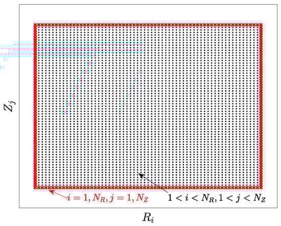
Figure 2. Illustration of a rectangular grid, where the red ‘x’s denote the boundary of the mesh while the black dots represents the core region.

In a tokamak, the boundary $\psi (R_{bd},Z_{bd})$ depends on the induced $\psi$ by the toroidal plasma current and conductor coil currents:

$$\begin{array}{cc}\hfill {\psi }^n(R_{bd},Z_{bd})& =({\int }_{{\mathsf{\Omega }}_{pl}}G(R_{bd},Z_{bd};R^{″},Z^{″})J_{\varphi ,pl}^n(R^{″},Z^{″})d{\mathsf{\Omega }}^{″}\hfill \\ \hfill & +\sum _{c=1}^{N_{coil}}G(R_{bd},Z_{bd};R_c,Z_c)·I_c^n)/\left(2\pi \right).\hfill \end{array}$$

(18)

Here $J_{\varphi ,pl}^n(R^{″},Z^{″})$ changes in each Picard iteration, while $I_c^n(R_c,Z_c)$ may either change or remain constant depending on the computational mode (forward vs. inverse), as discussed in Section 2.6.

2.5. Identification of Plasma Axis and Boundary

The determination of ${\psi }_{ax}$ and ${\psi }_{bd}$ in each Picard iteration is crucial since the nonlinear RHS of $J_{{\varphi }_{j,i}}$ strongly relies on ${\psi }_{ax}$ and ${\psi }_{bd}$. In a tokamak, the plasma boundary is either in contact with the plasma-facing component, e.g., the so-called limited or circular plasma shape, or formed by the saddle point of the poloidal magnetic field as an X-point (diverted plasma shape). Identifying ${\psi }_{ax}$ is relatively straightforward because it has the largest absolute value of $\psi$ inside the plasma area. On the other hand, determining ${\psi }_{bd}$ for a limited shape is also straightforward, as it is recognized by the existence of a closed contour, based on locating the maximum $\psi$ on the first wall coordinates. However, for a diverted plasma shape with an X-point, where a null magnetic field exists, the plasma boundary is identified by computing ${|\nabla \psi |}^2$.

Both the magnetic axis and X-points are characterized by local minima in ${|\nabla \psi |}^2$. Therefore, it is necessary to find the possible X-points and magnetic axis by calculating the following term:

$$S^{\prime }(R,Z)\equiv \left({\displaystyle \frac{{\partial }^2\psi }{\partial R^2}}\right)\left({\displaystyle \frac{{\partial }^2\psi }{\partial Z^2}}\right)-{\left({\displaystyle \frac{{\partial }^2\psi }{\partial R\partial Z}}\right)}^2,$$

(19)

along the magnetic axis, the maximum value of $\psi (R,Z)$ holds the same sign as for $({\partial }^2\psi /\partial R^2)$ and $({\partial }^2\psi /\partial Z^2)$, while they are opposite to each other when it is a saddle point (X-point) [23]. Therefore, the Hessian of $S^{\prime }>0$ indicates a magnetic axis, and $S^{\prime }<0$ indicates an X-point. The precise $(R,Z)$ coordinates for ${\psi }_{ax}$ and the X-points are determined using a new $\psi (R,Z)$ with small values of ($\delta R,\delta Z$). Although there may be multiple X-points, it is essential to identify the one that defines the plasma boundary and is closest to the plasma axis, as distinguished by having the maximum $\left|\psi \right|$.

2.6. Forward and Inverse Free-Boundary Equilibrium Modes

Within COTES, two computational modes are employed, namely, the forward and inverse modes. In the forward mode, the coil currents are known and remain fixed until a converged $\psi (R,Z)$ map is achieved. In contrast, the inverse mode treats the external coil currents as unknowns, which can be determined by additional constraints, e.g., the prescribed plasma boundary and X-points. In this inverse COTES approach, potential coil currents are explored by solving the following optimal problem:

$$\begin{array}{cc}\hfill \underset{\mathsf{\Delta }{I}_{coil}}{min}[& \sum _{e=1}^{N_{bnd}}{\left\{\sum _{c=1}^{N_{coil}}\left(G(R_e^{ref},Z_e^{ref};R_c,Z_c)·\mathsf{\Delta }{I}_{coil,c}\right)-\mathsf{\Delta }\psi (R_e^{ref},Z_e^{ref})\right\}}^2\hfill \\ \hfill +& \sum _{d=1}^{N_{Xpt}}{\left\{\sum _{c=1}^{N_{coil}}\left(G_{B_R}(R_d^{ref},Z_d^{ref};R_c,Z_c)·\mathsf{\Delta }{I}_{coil,c}\right)-B_R(R_d^{ref},Z_d^{ref})\right\}}^2\hfill \\ \hfill +& \sum _{d=1}^{N_{Xpt}}{\left\{\sum _{c=1}^{N_{coil}}\left(G_{B_Z}(R_d^{ref},Z_d^{ref};R_c,Z_c)·\mathsf{\Delta }{I}_{coil,c}\right)-B_Z(R_d^{ref},Z_d^{ref})\right\}}^2+{\gamma }^2\sum _{c=1}^{N_{coil}}{\left(\mathsf{\Delta }{I}_{coil,c}\right)}^2],\hfill \end{array}$$

(20)

where $(R_e^{ref},Z_e^{ref})$ are the specified boundary points; $G(R_e^{ref},Z_e^{ref};R_c,Z_c)$ is the Green’s function of the unit coil current $(R_c,Z_c)$ on the plasma boundary; $\mathsf{\Delta }\psi (R_e^{ref},Z_e^{ref})={\psi }_{bd}-\psi (R_e^{ref},Z_e^{ref})$ is the error of the poloidal flux function on the prescribed plasma boundary points; $B_R(R_d^{ref},Z_d^{ref})$ and $B_Z(R_d^{ref},Z_d^{ref})$ are the radial and vertical poloidal magnetic field on the given X-points $(R_d^{ref},Z_d^{ref})$, respectively; and $\gamma$ is a Tikhonov parameter for the regularization term [24] in an ill-posed problem. If an X-point is specified, then $B_R(R_d^{ref},Z_d^{ref})$ and $B_Z(R_d^{ref},Z_d^{ref})$ at the X-points should be zero. This constraint is added as the second and third summed terms in Equation (20), with

$$\begin{array}{cc}\hfill G_{B_R}& \equiv -{\displaystyle \frac{1}{R}}{\displaystyle \frac{\partial G}{\partial Z}}\hfill \\ \hfill G_{B_Z}& \equiv {\displaystyle \frac{1}{R}}{\displaystyle \frac{\partial G}{\partial R}}.\hfill \end{array}$$

(21)

The external coil currents for the next iteration are updated as

$$I_{coil,c}^{\left(n\right)}=I_{coil,c}^{(n-1)}+\mathsf{\Delta }{I}_{coil,c},$$

(22)

where $I_{coil,c}^{(n-1)}$ is the c-$th$ coil current from the $(n$−$1)th$ Picard iteration. It is important to emphasize that the initial $I_{coil}^0$ must be close to a real solution; otherwise, the Picard iteration will fail due to the absence of a possible plasma boundary and axis.

The solution to Equation (20) involves a least-squares regression with an L2 [25] penalty term, and the optimal coil currents are computed by

$$\begin{array}{cc}\hfill \mathsf{\Delta }{I}_{coil}^{opt}=& (G{(R_e^{ref},Z_e^{ref};R_c,Z_c)}^T·G(R_e^{ref},Z_e^{ref};R_c,Z_c)\hfill \\ \hfill & +G_{B_R}{(R_d^{ref},Z_d^{ref};R_c,Z_c)}^T{G}_{B_R}(R_d^{ref},Z_d^{ref};R_c,Z_c)\hfill \\ \hfill & +G_{B_Z}{(R_d^{ref},Z_d^{ref};R_c,Z_c)}^T{G}_{B_Z}(R_d^{ref},Z_d^{ref};R_c,Z_c)+{\gamma }^2·diag\left(\mathrm{I}\right){)}^{-1}\hfill \\ \hfill & \times (G{(R_e^{ref},Z_e^{ref};R_c,Z_c)}^T·\mathsf{\Delta }\psi (R_e^{ref},Z_e^{ref})\hfill \\ \hfill & +G_{B_R}{(R_d^{ref},Z_d^{ref};R_c,Z_c)}^T·B_R(R_d^{ref},Z_d^{ref})\hfill \\ \hfill & +G_{B_Z}{(R_d^{ref},Z_d^{ref};R_c,Z_c)}^T·B_Z(R_d^{ref},Z_d^{ref})).\hfill \end{array}$$

(23)

In practical exercises, when the value of $\gamma$ is fixed, the Picard iteration often encounters difficulty with convergence. It typically oscillates around a value significantly higher than the stop criterion ${ϵ}_b\sim {10}^{-4}$. To address this issue, it becomes necessary to reduce the regularization term on coil currents in Equation (20) by using a sequence of values for $\gamma$ [12]:

$${\gamma }^{n+1}={\gamma }^n{({ϵ}_b/{ϵ}_n)}^{1/2},$$

(24)

where

$${ϵ}_n\equiv \left|\right|\sum _{c=1}^{N_{coil}}\left(G(R_e^{ref},Z_e^{ref};R_c,Z_c)·\mathsf{\Delta }{I}_{coil,c}-\mathsf{\Delta }\psi (R_e^{ref},Z_e^{ref})\right)\left|\right|/|{\psi }_{bd}-{\psi }_{ax}|.$$

(25)

The iteration is stopped when ${ϵ}_n<={ϵ}_b$, which usually takes less than twenty iterations.

The detailed block diagram for the Picard iteration is illustrated in Figure 3. The dashed box highlights the process of determining the coil currents within the inverse mode. The diagram illustrates the Picard iteration process in the COTES code for solving the free-boundary equilibrium in the axisymmetric tokamak geometry. The process begins with an initial guess of the current density, $J_{\varphi ,j,i}^0$. This initial guess is used to calculate the boundary flux function, ${\psi }^0(R_{bd},Z_{bd})$, and the core flux function, ${\psi }^0(R_{core},Z_{core})$.

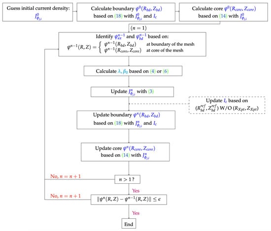
Figure 3. Block diagram of the Picard iteration in the COTES code. The diagram provides a representation of the iterative procedure and the conditions for updating the flux functions and current densities until convergence is achieved.

The iteration process starts with $n=1$. In each iteration, the values of ${\psi }_{ax}^{n-1}$ and ${\psi }_{bd}^{n-1}$ are identified. Then, the parameters $\lambda$ and ${\beta }_0$ are calculated based on the specified equations. The current density $J_{\varphi ,i}^n$ is updated accordingly.

Next, the boundary flux, ${\psi }^n(R_{bd},Z_{bd})$, and the core flux, ${\psi }^n(R_{core},Z_{core})$, are recalculated using the updated current density. If the inverse mode is selected, the coil currents $I_c$ are updated based on additional constraints.

The iteration continues with n being incremented by one each time. The process checks whether $n>1$ and whether the norm of the difference between the current and previous flux functions is within a specified tolerance $ϵ$. If the convergence criteria are met, the iteration ends; otherwise, it repeats.

2.7. Vertical Position Instability in Forward Mode

In the forward mode of COTES, the Picard iteration exhibits vertical instability, especially in cases where the plasma shape is asymmetric, such as the lower or upper single null (LSN or USN) X-point configuration. In previous work [12], a traditional approach to tackle this vertical excursion is to add a pair of fictitious feedback coils with currents:

$$I_{feedback}=-\mathrm{sign}\left(Z_{coil}\right)\left(C_1(Z_{ax}^n-Z_{desired})+C_2(Z_{ax}^n-Z_{ax}^{n-1})\right)·I_p,$$

(26)

where $Z_{coil}$ is the vertical coordinate of the fictitious feedback coil and $Z_{desired}$ is the target vertical position. This method works like a proportional and derivative (PD) controller, in which $C_1$ and $C_2$ are the P and D gains, respectively. However, a notable drawback of this technique is that the introduction of additional feedback coil currents inevitably alters the resulting $\psi (R,Z)$ map. Furthermore, the determination of $C_1$ and $C_2$ typically relies on trial and error.

Another treatment [11] also relies on adjusting the feedback coil currents to control the radial magnetic field $B_R$, which has a significant impact on the vertical instability. The corresponding feedback coil current is defined as follows:

$$I_{feedback}=-g_z{\displaystyle \frac{B_{R,Vac}}{B_{R,FB}^{*}}}{|}_{R_{cur},Z_{cur}},$$

(27)

where $g_z$ is an adjustable variable $\in [2,2.5]$; $B_{R,Vac}$ and $B_{R,FB}^{*}$ are the radial magnetic fields due to only the external coil currents and unit feedback coil current, respectively; and ($R_{cur},Z_{cur}$) is the effective barycenter of the plasma current. By this approach, guessing the vertical desired position is not necessary, but additional coil currents can also change the converged $\psi (R,Z)$ map.

In this work, a sophisticated approach without feedback coil currents was implemented. Instead of adding fictitious feedback coils, the current density $J_{\varphi j,i}$ was adjusted by

$$\begin{array}{cc}\hfill \chi & =K_p(Z_{desired}-Z_{ax}),\hfill \\ \hfill J_{\varphi j,i}^{n,new}& =(1-\chi )J_{\varphi j,i}^{n,old}+\chi \left(J_{\varphi j,i}^{n,old}{\displaystyle \frac{\partial diag{\left(I\right)}_{j,i}}{\partial Z}}\right),\hfill \end{array}$$

(28)

where $J_{\varphi j,i}^{n,old}$ is the plasma current density in the n-$th$ Picard iteration in Figure 3 based on ${\psi }_{j,i}^{n-1}$, $\chi \in [-1,1]$ is a relaxing factor, and $K_p$ is an adjusted control parameter. On the other hand, $J_{\varphi j,i}^{n,new}$ represents the modified current density used for the ${\psi }_{j,i}^n$ calculation. The advantage is that no extra coil currents are needed to modify the final $\psi (R,Z)$ map, although it does necessitate an initial guess for $Z_{desired}$ prior to starting the Picard iteration. Similar methods are widely employed in the equilibrium reconstruction codes EFIT [13], CLISTE [26], and LIUQE [27].

3. Benchmarks and Numerical Verifications

This section discusses a series of benchmarks and verifications for COTES simulations. To ensure mathematical correctness and accuracy, COTES is directly compared against an analytical fixed-boundary equilibrium solution. Furthermore, additional benchmark tests are conducted using another numerical solver with a distinct computational grid and method. Finally, the numerical results obtained from COTES are verified by comparing them with the equilibrium reconstruction code EFIT, which is based on the DIII-D low (L) confinement experimental data.

3.1. Benchmark with Analytic Fixed-Boundary Equilibrium Solver

To assess the mathematical correctness and accuracy of the COTES simulation, a recently developed analytic fixed-boundary equilibrium solver [4] was applied as a benchmark. The pressure and toroidal current density in this analytic solver are defined as follows:

$$\begin{array}{cc}\hfill p\left(\psi \right)& =p_0{\left({\displaystyle \frac{\psi }{{\psi }_0}}\right)}^2,f^2\left(\psi \right)=R_0^2{B}_{{\varphi }_0}^2\left[1+{\displaystyle \frac{2\delta B}{B_{{\varphi }_0}}}{\left({\displaystyle \frac{\psi }{{\psi }_0}}\right)}^2\right],\hfill \end{array}$$

(29a)

$$\begin{array}{cc}\hfill J_{\varphi ,pl}& =R{\displaystyle \frac{dp\left(\psi \right)}{d\psi }}+{\displaystyle \frac{1}{2{\mu }_{0}R}}{\displaystyle \frac{d{f}^2\left(\psi \right)}{d\psi }},\hfill \end{array}$$

(29b)

where ${\psi }_0$ is the poloidal flux function on the magnetic axis, $p_0$ is the kinetic pressure on the axis, and $\delta B/B_{{\varphi }_0}$ is a measure of the toroidal field diamagnetism on the axis. In this approach, all the plasma parameters, such as p, $p^{\prime }$, and f, as well as $\psi$, vanish on the plasma boundary surface, i.e., $\psi \left(\mathrm{surf}\right)=0$.

The prescribed plasma boundary is defined by the Miller profile [28]. The fixed plasma boundary, $(R_S,Z_S)$, is given in terms of an angle-like parameter $\theta$, $\theta \in [0,2\pi ]$, as

$$R_S=R_0+acos(\theta +\widehat{\delta }sin\theta ),Z_S=a\kappa sin\theta ,$$

(30)

in which $\kappa$ is the elongation, $\delta$ is the triangularity, and $\widehat{\delta }=si{n}^{-1}\delta$.

The benchmark was carried out with the assumption that both the inverse mode of COTES and the analytic solver shared an identical plasma boundary, which was defined by $\kappa =1.45$, $\delta =0.2$, $R_0=1.81$m, and $a=0.4$m. The values $I_p=0.68MA$, ${\beta }_p=0.5$, and $B_{{\varphi }_0}=2.0T$ were prescribed. Iso$-{\psi }_N$ contours ranging from 0 to 1 with a step of 0.1 are shown in Figure 4.

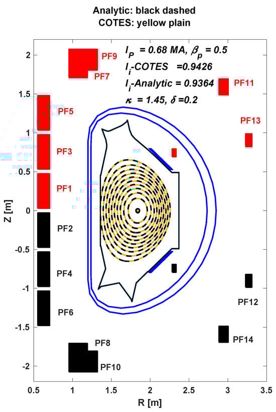
Figure 4. Iso$-{\psi }_N\in$ (0:0.1:1) contour comparisons between the inverse of COTES (yellow plain) and the analytic (black dashed) fixed-boundary equilibrium solver with an EAST geometry.

A remarkable observation was that the iso$-{\psi }_N$ contours aligned perfectly, which extended from the plasma boundary to the axis. This excellent agreement along the plasma axis can be attributed to the combined effects of ${\beta }_p+l_i/2$, referred to as the Shafranov shift. Here, $l_i$ denotes the plasma internal inductance, which characterizes the peaking of the current density distribution. The ${\beta }_p$ in both the analytic and inverse numerical solvers were forced to 0.5, resulting in $l_i$ with 0.9364 and 0.9462, respectively, which, in turn, yielded almost the same ${\beta }_p+l_i/2$. These well-matched iso$-{\psi }_N$ contours between COTES and the analytic fixed-boundary solver underscore the high credibility of both solvers in terms of their mathematical correctness and accuracy.

3.2. Verifications with Numerical Free-Boundary Equilibrium Solver

A comparison analysis was undertaken between the COTES simulation results and those from the numerical FBE solver FEEQS.M to make sure that the COTES simulation was correct and accurate. FEEQS.M employs the finite element method and Newton-type iteration on a triangular-based grid. The simulations herein were carried out using the EAST [29] geometry.

The different computational grids for COTES and FEEQS.M are illustrated in Figure 5. In COTES, the rectangular domain spanned $[R_{min},R_{max}]\in [1.2,2.6]$m and $[Z_{min},Z_{max}]\in [-1.2,1.2]$m, with $N_R=N_Z=65$, while for FEEQS.M, the computational domain was a semi-circular area with radius $r=3.5$m, and the sizes of the triangles in different areas were adjusted to reduce the total number of elements.

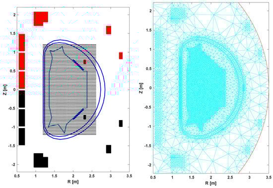
Figure 5. (Left): rectangular grid in COTES. (Right): triangular grid with finite element method in FEEQS.M code.

The verification process aligned with the benchmark described in Section 3.1, i.e., both numerical approaches were executed by inverse modes and shared the same plasma boundaries (limited and X-point diverted configurations). For simplicity, the $J_{\varphi ,pl}$ in both codes applied the same polynomial functions as specified in Equation (3). The $l_i$ was tuned by trial and error with different ${\alpha }_n$ and ${\beta }_n$ in Equation (3b).

The verified results, including the plasma parameters and internal profiles for the limited configuration, are shown in Figure 6. The overlapped iso$-{\psi }_N$ contours signify that the numerical solutions obtained through different methods, encompassing variations in the computational grid, discrete approximations, and iterative processes, were in complete agreement. In addition to the ${\psi }_N$ contours, the plasma internal profiles, particularly q and $J_{\varphi ,pl}$ computed by distinct numerical integrals, also exhibited a perfect overlap. This consistency underscored the correctness and accuracy of both numerical methods.

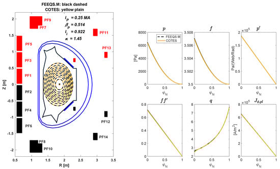
Figure 6. (Left): iso$-{\psi }_N\in$(0:0.1:1) contour plots comparisons between inverse of COTES (yellow plain) and FEEQS.M (black dashed) solutions. (Right): plasma internal profiles of $p,f,p^{\prime },f{f}^{\prime },q$, and $J_{\varphi ,pl}$ in COTES (plain) and FEEQS.M (dashed).

To further verify the agreement between these two numerical FBE solutions, inverse calculations with the LSN configuration were compared, and the results are presented in Figure 7. Once again, the iso$-{\psi }_N$ contour plots displayed a flawless overlap. However, some slight discrepancies were observed in the plasma profiles, particularly for $p,f,p^{\prime }$, and $f{f}^{\prime }$. These minor variations suggest that in the asymmetric plasma configuration, differences between the two numerical methods can arise, though overall agreement is maintained.

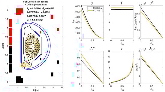
Figure 7. (Left): iso$-{\psi }_N\in$ (0:0.1:1) contour plot comparisons between the inverse of COTES (yellow plain) and FEEQS.M (black dashed) solutions. (Right): plasma internal profiles of $p,f,p^{\prime },f{f}^{\prime },q$, and $j_{\varphi ,pl}$ in COTES (plain) and FEEQS.M (dashed).

3.3. Verification with Equilibrium Reconstruction Data

COTES FBE solutions can be compared with plasma equilibrium reconstructions from experiments based on diagnostic measurements. In the EFIT code [13], coil currents are given, but the toroidal plasma current density is unknown and must be determined. The toroidal current density can be inferred based on constraints from experimental measurements, such as the magnetic field and flux. The optimization objective to minimize is

$${\chi }^2=\sum _{k=1}^{N_{meas}}{\left({\displaystyle \frac{M_k-C_k}{{\sigma }_k}}\right)}^2,$$

(31)

where $M_k,C_k$, and ${\sigma }_k$ are the experimental measurement, calculated value, and associated error for the k-$th$ term, respectively. The pressure and diamagnetic function for the calculation of $J_{\varphi ,pl}$ for the equilibrium construction is defined as

$$p^{\prime }\left({\psi }_N\right)=\sum _{n=0}^{n_p}{a}_n{\left({\psi }_N+{\displaystyle \frac{\partial {\psi }_N}{\partial Z}}\delta Z\right)}^n;f{f}^{\prime }\left({\psi }_N\right)=\sum _{n=0}^{n_f}{b}_n{\left({\psi }_N+{\displaystyle \frac{\partial {\psi }_N}{\partial Z}}\delta Z\right)}^n,$$

(32)

where $a_n$ and $b_n$ are unknown constants, and $\delta Z$ is an approximated rigid vertical shift of the ${\psi }_N$ distribution used to adjust the vertical position.

The DIII-D [30] L mode shot 157952 at 1300 ms was selected as the case for comparison. This particular shot corresponds to an LSN X-point divertor configuration, which naturally experiences vertical instability during the Picard iteration in the forward mode. Consequently, all three approaches described in Section 2.6 were compared against the EFIT result, as it is shown in Figure 8. Generally, all three methods exhibited similar plasma boundaries when compared with the EFIT result. The alignment with the EFIT axis was particularly close for the approaches described in Equations (26) and (28), given that the EFIT axis served as the target in both cases.

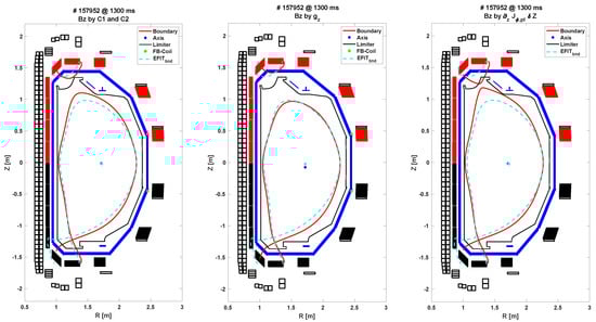
Figure 8. The plasma boundary between EFIT (cyan dashed) and the forward of COTES (red plain) with three vertical instability approaches.

However, there were also some discrepancies observed between the EFIT result and the forward mode of COTES, especially in terms of the X-point position. Several factors could contribute to these differences. First, the induced current on the vacuum vessel is not currently considered in COTES, whereas EFIT includes these currents in its reconstruction. Second, the EFIT result involves determining the constants $a_n$ and $b_n$ in Equation (32) to match the experimental measurements of magnetics, which may have associated error bars. Lastly, the plasma internal profiles (p and f) between EFIT and COTES are different, just as depicted in Figure 9.

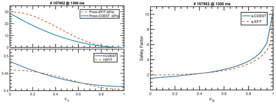
Figure 9. (Left): profiles of p and f between EFIT (dashed) and COTES (plain) simulations. (Right): profile of q between EFIT (dashed) and COTES (plain) simulations.

4. Conclusions and Future Work

In this study, the free-boundary equilibrium problem in axisymmetric tokamak geometry was addressed using the COTES code by employing the finite difference method with Picard iteration. COTES discretizes the 2D partial differential equation over a rectangular domain through finite difference approximations. The nonlinear toroidal plasma current density starts from an initial guess and is then defined as a polynomial function based on the ${\psi }_{ax}$ and ${\psi }_{bd}$ from the previous iteration, as well as plasma quantities, such as $I_p$ and ${\beta }_p$ or $q\left({\psi }_N\right)$. COTES can run either in a forward mode, where the coil currents are fixed, or in an inverse mode, where the coil currents are calculated in every iteration based on a prescribed plasma boundary with an optimal control approach. To address the vertical instability issues that occurred in the forward mode for the asymmetric plasma shape, a vertical shift of $J_{\varphi ,pl}$ instead of adding feedback coils, as used in previous work, was employed.

For benchmarking and verification, COTES simulations were initially compared with an analytic fixed-boundary solver to verify the mathematical correctness and accuracy. The results demonstrate excellent agreement in the internal flux surface profiles. Subsequently, the COTES simulations were cross-checked with another numerical solver, FEEQS.M, which employs different approximations and computational grids. The findings show that COTES yielded consistent solutions in the limiter configuration and similar plasma internal profiles in the X-point plasma boundary when compared with the FEEQS.M simulations. Finally, the COTES simulations were verified against the equilibrium reconstruction code EFIT using experimental data to assess its capability to handle vertical instability through different approaches. The discrepancies between the COTES and EFIT results were also explained through potential interpretations.

Future work on COTES involves coupling it with circuit equations for external coil systems, encompassing a vacuum vessel and passive plates, to tackle the FBE problems in time evolution rather than static modes. Another direction for advancing COTES is exploring surrogate models for the toroidal current density derived from experimental measurements or other transport solvers, instead of using given polynomials.

References

- LoDestro, L.L.; Pearlstein, L.D. On the Grad–Shafranov equation as an eigenvalue problem, with implications for q solvers. Phys. Plasma 1994, 1, 90. [Google Scholar] [CrossRef]
- Zheng, S.B.; Wootton, A.J.; Solano, E.R. Analytical tokamak equilibrium for shaped plasmas. Phys. Plasma 1996, 3, 1176. [Google Scholar] [CrossRef]
- Cerfon, A.J.; Freidberg, J.P. “One size fits all” analytic solutions to the Grad–Shafranov equation. Phys. Plasma 2010, 17, 032502. [Google Scholar] [CrossRef]
- Guazzotto, L.; Freidberg, J.P. Simple, general, realistic, robust, analytic tokamak equilibria. Part 1. Limiter and divertor tokamaks. J. Plasma Phys. 2021, 87, 905870303. [Google Scholar] [CrossRef]
- Heumann, H.; Blum, J.; Boulbe, C.; Faugeras, B.; Selig, G.; Ané, J.-M.; Brémond, S.; Grandgirard, V. Quasi-static free-boundary equilibrium of toroidal plasma with CEDRES++: Computational methods and applications. J. Plasma Phys. 2015, 81, 905810301. [Google Scholar] [CrossRef]
- Blum, J.; Heumann, H.; Nardon, E.; Song, X. Automating the design of tokamak experiment scenarios. J. Comp. Phys. 2019, 394, 594–614. [Google Scholar] [CrossRef]
- Nardon, E.; Heumann, H. Magnetic configuration and plasma start-up in the WEST tokamak. In Proceedings of the 45th EPS Conference on Plasma Physics, Prague, Czech Republic, 26 October 2018. [Google Scholar]
- Song, X.; Nardon, E.; Heumann, H.; Faugeras, B. Automatic identification of the plasma equilibrium operating space in tokamaks. Fusion Eng. Des. 2019, 146, 1242. [Google Scholar] [CrossRef]
- JET Team. Fusion energy production from a deuterium-tritium plasma in the JET tokamak. Nucl. Fusion 1992, 32, 187. [Google Scholar] [CrossRef]
- Jardin, S.C.; Bell, M.G.; Pomphrey, N. TSC simulation of Ohmic discharges in TFTR. Nucl. Fusion 1993, 33, 371. [Google Scholar] [CrossRef]
- Jeon, Y.M. Development of a Free-boundary Tokamak Equilibrium Solver for Advanced Study of Tokamak Equilibria. J. Korean Phys. Soc. 2015, 67, 843–853. [Google Scholar] [CrossRef]
- Johnson, J.L.; Dalhed, H.E.; Greene, J.M.; Grimm, R.C.; Hsieh, Y.Y.; Jardin, S.C.; Manickam, J.; Okabayashi, M.; Storer, R.G.; Todd, A.M.; et al. Numerical Determination of Axisymmetric Toroidal Magnetohydrodynamic Equilibria. J. Comp. Phys. 1979, 32, 212–234. [Google Scholar] [CrossRef]
- Ferron, J.R.; Walker, M.L.; Lao, L.L.; John, H.E.S.; Humphreys, D.A.; Leuer, J.A. Real time equilibrium reconstruction for tokamak discharge control. Nucl. Fusion 1998, 38, 1055. [Google Scholar] [CrossRef]
- Shafanov, V.D. On magnetohydrodynamical equilibrium configurations. Sov. Phys. JETP 1958, 8, 494. [Google Scholar]
- Grad, H.; Rubin, H. Hydromagnetic equilibria and force-free fields. In Proceedings of the 2nd UN Conference on the Peaceful Uses of Atomics Energy, Geneva, Switzerland, 1 September–13 September 1958; Volume 31, p. 190. [Google Scholar]
- Lazarus, E.A.; Lister, J.B.; Neilson, J.H. Control of the vertical instability in tokamaks. Nucl. Fusion 1990, 30, 111. [Google Scholar] [CrossRef]
- Albanese, R.; Villone, F. The linearized CREATE-L plasma response model for the control of current, position and shape in tokamaks. Nucl. Fusion 1998, 38, 012001. [Google Scholar] [CrossRef]
- Blum, J.; Boulbe, C.; Faugeras, B. Reconstruction of the equilibrium of the plasma in a Tokamak and identification of the current density profile in real time. J. Comp. Phys. 2012, 231, 960–980. [Google Scholar] [CrossRef]
- William, H.P. Numerical Recipes; The Art of Scientific Computing, 3rd ed.; Cambridge University Press: New York, NY, USA, 2007. [Google Scholar]
- Kreyszig, E. Advanced Engineering Mathematics, 8th ed.; John Wiley & Sons Press: Hoboken, NJ, USA, 1998. [Google Scholar]
- Jardin, S. Computational Methods in Plasma Physics, 1st ed.; Taylor & Francis CRC Press: New York, NY, USA, 2010. [Google Scholar]
- Miyamoto, K. Plasma Physics for Nuclear Fusion, revised ed.; The MIT Press: Cambridge, MA, USA, 1989. [Google Scholar]
- Quarteroni, A.; Sacco, R.; Fausto, S. Numerical Mathematics; Springer Science & Business Media: New York, NY, USA, 2010; Volume 37. [Google Scholar]
- Tikhonov, A.N.; Arsenin, V.Y. Solutions of Ill-Posed Problems; Winston & Sons: Washington, DC, USA, 1977. [Google Scholar]
- Thrampoulidis, C.; Oymak, S.; Hassibi, B. Regularized linear regression: A precise analysis of the estimation error. In Proceedings of the Machine Learning Theory (PMLR), Lille, France, 3–6 July 2015; pp. 1683–1709. [Google Scholar]
- McCarthy, P.J.; Martin, P.; Schneider, W. The CLISTE Interpretive Equilibrium Code; Tech. Rep. IPP 5/85; Max Planck Institute for Plasma Physics: Greifswald, Germany, 1999. [Google Scholar]
- Moret, J.M.; Duval, B.P.; Le, H.B.; Coda, S.; Felici, F.; Reimerdes, H. Tokamak equilibrium reconstruction code LIUQE and its real time implementation. Fusion Eng. Des. 2015, 91, 1–15. [Google Scholar] [CrossRef]
- Miller, R.L.; Chu, M.S.; Greene, J.M.; Lin-Liu, Y.R. Noncircular, finite aspect ratio, local equilibrium model. Phys. Plasma 1998, 5, 973. [Google Scholar] [CrossRef]
- Wu, S.T.; The EAST Team. An overview of the EAST project. Fusion Eng. Des. 2007, 82, 463–471. [Google Scholar] [CrossRef]
- Luxon, J.L. A design retrospective of the DIII-D tokamak. Nucl. Fusion 2002, 42, 614. [Google Scholar] [CrossRef]
Disclaimer/Publisher’s Note: The statements, opinions and data contained in all publications are solely those of the individual author(s) and contributor(s) and not of MDPI and/or the editor(s). MDPI and/or the editor(s) disclaim responsibility for any injury to people or property resulting from any ideas, methods, instructions or products referred to in the content. |
© 2024 by the authors. Licensee MDPI, Basel, Switzerland. This article is an open access article distributed under the terms and conditions of the Creative Commons Attribution (CC BY) license (https://creativecommons.org/licenses/by/4.0/).