Modeling of Energy Consumption and Print Time for FDM 3D Printing Using Multilayer Perceptron Network

Abstract

Given the recognized advantages of additive manufacturing (AM) printing systems in comparison with conventional subtractive manufacturing systems, AM technology has become increasingly adopted in 3D manufacturing, with usage rates increasing dramatically. This strong growth has had a significant and direct impact not only on energy consumption but also on manufacturing time, which in turn has generated significant costs. As a result, this problem has attracted the attention of industry actors and the research community, and several studies have focused on predicting and reducing energy consumption and additive manufacturing time, which has become one of the main objectives of research in this field. However, there is no effective model yet for predicting and optimizing energy consumption and printing time in a fused deposition modeling (FDM) process while taking into account the correct part orientation that minimizes both of these costs. In this paper, a neural-network-based model has been proposed to solve this problem using experimental data from isovolumetrically shaped mechanical parts. The data will serve as the basis for proposing the appropriate model using a specific methodology based on five performance criteria with the following statistical values: R2-squared > 99%, explained variance > 99%, MAE < 0.99%, MSE < 0.02% and RMSE < 1.36%. These values show just how effective the proposed model will be in estimating energy consumption and FDM printing time, taking into account the best choice of part orientation for the lowest cost. This model provides a global understanding of the primary energy and time requirements for manufacturing while also improving the system’s cost efficiency. The results of this work can be extended and applied to other additive manufacturing processes in future work.

1. Introduction

According to the Wohlers 2023 report, global growth in additive manufacturing products and services is estimated at 18.3%, with double-digit growth recorded over the past 34 years. The statistics from the same report confirm that there is a remarkable growth in materials, software, 3D printing services and hardware, with this growth rate being estimated at 23% in 2022 [1]. However, due to the large number of machines and production efficiency, the AM process has a low energy efficiency. In particular, for a short grinding process with long pauses, the energy consumption is higher, and the running time is more considerable [2]. This is why it has become crucial to design solutions that lead to optimized energy consumption for AM systems. Moreover, AM systems have a negative impact on the environment, and their effects can even have detrimental potential [3,4]. The study of energy consumption is useful for selecting the appropriate strategy and choosing the parameters to be adopted in 3D manufacturing. These parameters may be related to product design or shape accuracy but also to physical, mechanical, electrical, or thermal parameters [5].

In an additive manufacturing process, parts are formed by creating consecutive layers, with each layer representing a cross-section of the part. This process is based on CAD data transmitted to the additive manufacturing printing system [3,6,7,8]. On the other hand, there are seven types of additive manufacturing processes, classified on the basis of machine architecture. In addition, a number of standards are recommended for additive manufacturing, and to this end, an ASTM F42 committee meets twice a year to publish AM standards while also presenting work in progress. These standards help manufacturing specialists and machine manufacturers [9,10]. The seven processes of AM include the following: The vat photopolymerization (VPP) process uses liquid polymers that react to radiation by solidifying and ultraviolet light, which solidifies the liquid into layers. Powder bed fusion (PBF) is considered one of the most versatile manufacturing processes, as it can be applied to metals and polymers to a lesser extent. This process uses a container filled with powder that is selectively treated with an energy source, typically a scanning laser or electron beam. The material jetting process (MJT) generally uses materials in a viscous state. It consists of selectively placing droplets of raw material on a platform, after which UV light is applied to create the first layer. This process continues with the creation of other consecutive layers and stops when the final part is formed. In the binder jetting (BJT) process, a bed with a layer of fine particles in powder form is used by selectively depositing a liquid binder to build up the high-value parts. This process is carried out by creating one layer after another, and at each stage, a cross-section of the part is formed. Sheet lamination is a process that joins sheets of material together to form a part, and the manufacturing process is performed by ultrasonic welding. Directed energy deposition (DED) is a directed process, since the melting of materials is performed by applying thermal energy. This melting is performed once the material is deposited in the system. Material extrusion is a technology that typically uses a polymer as the thermoplastic material and a heated nozzle to build the layers. Material extrusion is a technology that generally uses a polymer as the thermoplastic material and a heated nozzle to build up the layers. In this class of extrusion technology, the most popular process is FDM, in which the polymer is deposited in the system as a filament, and this polymer is liquefied via a reservoir in a heated state. The filament is deposited by pushing it into the reservoir via a “pinch roller”, whose role is to generate the pressure that extrudes the material [10,11,12,13]. Among the seven additive manufacturing processes, FDM is commonly used in 3D printing due to its excellent mechanical properties and a wide choice of materials, including thermoplastic polymers, ceramics and low-melting metals [10,14].

AM technology has a number of advantages in industry, including being a provider of sustainability, offering the possibility of creating customized prototypes, producing less waste and carbon monoxide gas and promoting a circular economy [15]. In comparison with subtractive manufacturing and bulk forming, a number of studies have been carried out in this field. Yoon, Lee et al. [16] examined three types of manufacturing: additive manufacturing, subtractive processes and bulk forming. The comparison showed that additive manufacturing is 100 times more expensive than bulk forming. This study showed that subtractive manufacturing processes have intermediate costs between the other two categories, which vary over a wide range, but the processes also vary in terms of scale. The authors prove that the specific energy consumption of AM has a negative logarithmic correlation with productivity and concluded their study by pointing out that AM processes require more extensive evaluation of the environmental effect. David Rejeski [17] highlighted the potential environmental impacts of additive manufacturing, including waste generation, energy consumption, health risks, and life cycle impacts. In addition, the authors provided evidence that additive manufacturing technologies consume more energy than conventional manufacturing technologies. Other research comparing the energy consumption between AM processes and conventional printing methods has shown that the specific energy consumption (SEC) of AM is one to two times higher than that of conventional methods. Moreover, only part of the environmentally oriented taxonomy has been documented with regard to AM processes, and most work focuses on energy consumption [8]. In this sense, the issue of energy consumption in AM has attracted the attention of many researchers [18,19,20].

The technologies of AM could support intellectualization and industrialization; moreover, AM systems are more complex, with multiple factors (structure, materials with physical and chemical considerations, cost, etc.); therefore, it is essential to study these systems based on artificial intelligence and big-data techniques [21]. In this context, several studies have been carried out to model energy consumption using machine learning [22,23,24]. However, it should be noted that for an FDM manufacturing process, there is not yet a model for predicting energy consumption and printing time that provides good results for optimizing these two costs while taking into account correct part orientation.

In this study, modeling of the experimental results of the energy consumption and printing time of isovolumetric 3D mechanical parts was carried out by an artificial neural network (ANN)-based approach. The developed network estimates the FDM energy consumption and printing time with high accuracy, having an MSE value of 0.018%, an R2 Square value of 99.59%, an MAE value of 0.989%, an explained variance value of 99.60% and an RMSE value of 1.355%. In this context, this paper is organized as follows. It comprises several sections that collectively present a comprehensive study on the prediction of energy consumption and printing time in additive manufacturing. The Section 2 describes 4D FDM printing, and the Section 3 provides an overview of the existing research conducted in this field, offering insights into the work carried out thus far. Following that, the Section 4 delves into the description of the experimental data [25] and materials utilized, elucidating its relevance to the study at hand. Moving on to the Section 5, the paper outlines the methodology employed in this study, accompanied by a brief exposition on the algorithms utilized. In the subsequent Section 6, a comparison of the results of the models used in this study is presented. In the Section 7, the adopted modeling approach is detailed, shedding light on the techniques and strategies employed. The Section 8 engages in a comprehensive discussion of the results obtained from the study, analyzing and interpreting the findings. Finally, the Section 9 encapsulates the main conclusions derived from the research, along with highlighting potential avenues for future exploration.

2. FDM 4D Printing

With the progress recorded in the development of 4D printing, 4D additive manufacturing looks promising for future work [26,27]. This technology can be successfully applied to expand several composite structures with shape memory, as in the case of 4D printing with “bi-stable” structures featuring intelligent responses [28]. Shape-memory polymer materials have additional functional capabilities that enable fourth-dimensional production, since these polymer-based materials are stimuli-responsive and have the advantage of modifying their shapes after printing has been complete [29]. In this context, several studies have investigated the use of these polymers in 4D manufacturing.

Bodaghi et al. [26] used double-layer encapsulated polycaprolactone (PCL) and thermoplastic (TPU) shape-memory composite structures 4D-printed for the first time. SME performance is studied by examining “fixity”, “shape recovery”, “stress recovery” and “stress relaxation” under flexural and compressive loading modes. On the other hand, the melting temperature of the PCL material, PCL and TPU influence the transition temperature, switching and net point, respectively. Taking into account the destruction of PCL, the dripping of this molten material and its contact with water, TPU encapsulates PCL, and this encapsulation offers a solution to the interlayer “bond/interface” while surpassing in the SME performance the bilayer printing of PCL-TPU. Subsequent experiments have shown that composites manufactured in 4D have a maximum stress recovery that does not change over time. The modulus of elasticity of TPU at the melting temperature of PCL is 16.5 times higher than that of PCL, because the latter has not been adapted to resist the release of TPU force, since the material has a behavior that is elastic in loading and recovery. Moreover, in the three bilayer and encapsulated structures, we find that the shape recovery values are 100%. In the compressive stress shape memory test, the highest temperature yielded a maximum stress value that did not decrease with time. Compared with extrusion-based SMP structures, the result of this work solves the problem of poor stress relaxation of previous SMPs. In [30], an adaptive metamaterial design with performance directly integrated into materials was investigated using FDM technology. The idea is to understand the thermomechanics of shape-memory polymers and the advantages offered by FDM for programming metamaterials that are self-folding. In this sense, five parameters that can influence material adaptation have been studied: “material”, “platform surface”, “relay-time” for printing each layer, “temperature”, “printing speed” and “liquefier temperature”. Given that the self-folding characteristic affects the change in shape and programming layer by layer, experiments have been carried out to determine how printing speed and liquefier temperature can affect this characteristic. In addition, a finite element (FE) formulation was used to provide a customized description of the materials in both the manufacturing and deformation phases. In this context, the combination of FE and FDM solutions was used to create straight or curved beams as structural primitives with the characteristics of being self-bending and self-winding. This 4D printing study demonstrated that adaptive metamaterials can be used to create prototypes capable of transformation in 2D or 3D and in several fields. This gives the advantage of designing and developing functional structures that feature “self-folding”, “self-coiling”, “self-conforming” and “self-deploying features in a controllable manner”. In [31], the parameters influencing 4D printing were studied, and these parameters mainly concern the design of the structure, the material, programming during printing and activation. In this context, FDM technology has been used with thermoplastic polymers as shape-memory materials (SMPs). These SMPs are printed in temporary shapes and then transformed into permanent forms under the effect of heat. In addition, material selection depends mainly on the shape-memory behavior of the filaments, while design is complex because of the freedom of design, and print programming depends directly on the printing parameters. For polymer activation, there are various methods, such as Joule or infrared activation, and these depends on the “amplitude”, “duration”, “support of the stimulus” and “stimulus environment”. In addition, it has been shown that activation parameters influence the transformation process, so a longer exposure time generates a greater amount of transformation, which reaches its maximum as the stress relaxes. For the activation temperature, the higher the temperature, the higher the velocity and the greater the transformation. Finally, the authors confirm that planning, comparison and presentation of the structured design of experiments offer the presented 4D FDM model advantages in terms of long-term time savings.

The 4D FDM printing method is a futuristic technology that offers many advantages to the manufacturing industry. This type of manufacturing relies primarily on FDM and the ability of parts to transform their shape using advanced programmable materials. As a result, this technology needs to be studied closely, particularly in terms of resource consumption, which necessarily involves understanding the factors that influence the cost of manufacturing, in particular time and energy. The following section provides an overview of existing research on energy consumption and manufacturing time in the AM field.

3. Related Works

As research and industry focus on sustainable manufacturing increases, energy consumption in additive manufacturing processes is becoming an intriguing topic in the research community. In this sense, several studies have focused on modeling and optimizing the amount of energy consumed in additive manufacturing [18,19,20,32,33,34,35]. In the literature, studies of energy consumption have been carried out either using specific methods or based on machine learning techniques. In the following, several studies will be proposed on this subject.

Harding et al. [35] used six approaches to reduce energy and material consumption in filament fusion manufacturing (FFF). These approaches were studied using commercial printers, and the results show that energy consumption can be significantly reduced by insulating the hot end (33.8% to 30.63% reduction) and the sealed enclosure (18% power reduction). In contrast, 51% of the material was saved by using a type of “lightning infill”. Vidakis et al. [5] examined the parameters that influence three types of energy in 3D ABS-FFF manufacturing: specific printing energy (SPE), the energy printing consumption (EPC), and specific printing power (SPP). The authors studied the effect of six parameters on energy consumption: the infill raster density (ID), raster deposition angle (RDA), nozzle temperature (NT), fused filament printing speed (PS), layer deposition thickness (LT), and bed temperature (BT). As a result, PS and LT significantly influence EPC and SPE energy types. The density (ID), on the other hand, mainly influences SPP energy. In addition, an increase in layer thickness and printing speed can reduce EPC and SPE energies. This study uses quadratic regression models (QRM) and six-parameter ANOVA on the three energy types; however, these models are effective and sufficient for the two energy types SPE and EPC but not for the SPP energy type. Yang et Liu [36] presented an approach for predicting the energy consumption with material usage and print time of 3D-printed parts while relying on the path planning code and intrinsic characteristics of the machine. The authors proposed a method for predicting and reducing energy consumption in the prefabrication phase. The model developed in this study is suitable for several machines and other computer-aided manufacturing processes. Markos Petousis et al. [37] examined the impact of seven parameters (orientation angle, screen deposition angle, fill density, layer thickness, nozzle temperature, printing speed and bed temperature) on compression and energy consumption in a material extrusion process (MEX) using acrylonitrile butadiene styrene (ABS) as the material. In terms of energy consumption, the results of this study show that layer thickness and printing speed have the greatest impact. However, printing time was not included in this study. Helena Monteiro et al. [38] focused their study by undertaking a systematic literature review of metal additive manufacturing (MAM) processes in the aerospace and aeronautics sector. This analysis was based on literature classified according to four life cycle stages to identify efficiency strategies related to MAM resources. These stages concern “product design”, “materials development and sourcing”, “process development, control and optimization” and “end-of-life extension and circular economy”. The authors identify the key factors influencing the energy and material efficiency of this type of manufacturing. Zhiqiang Yan et al. [34] proposed a model to predict power consumption and printing time as a function of process parameters and machine component operating states. This model takes into account “the power of each component” and “the duration of each process”; however, this model has some limitations. The prediction of empty travel time, deceleration and acceleration of the nozzle movement are not supported by the model. Baumers, Tuck et al. [39] proposed a tool capable of predicting the energy flows that will occur in direct laser sintering of metals. This tool also estimates the costs of the process. It has been shown that minimizing costs in additive manufacturing can minimize the energy consumption of the process, thus motivating improvements in sustainability. Meteyer, Xu et al. [40] developed a model to evaluate the energy and material consumption for the binder jetting process. Mathematical studies determined the energy consumption depending on the printing parameters and the geometry of the part. To validate their model, test printing was performed. The resulting energy consumption model provides a tool for optimizing the geometric design of parts. Verma et Rai [41] developed an approach to optimize selective laser sintering (SLS) in stages to minimize energy consumption. In this study, the energy consumption and waste related to the materials used are reduced both in parts and in layers. The models developed in SLS can be applied to other AM processes; however, these models do not consider printing time and part orientation. Ajay et al. [23] proposed a unified FDM approach to optimization of “power between layers”, “instructions”, “hardware”, “compilers” and “firmware”. In addition, using the energy profiler, a solution called 3DGates was proposed to optimize interlayer energy, combining the instruction set, compiler and firmware. This solution was evaluated on 338 benchmarks, resulting in an energy reduction of 25%. Yiran Yang in [42] developed a mathematical model to predict energy consumption in stereolithography processes. The obtained results have been verified experimentally. In addition, an assessment of the impact of different parameters on the total energy consumption was conducted, and a method to reduce energy consumption was suggested based on an optimal combination of parameters. Simon et al. [43] conducted their study on the effect of certain printing parameters on particulate emissions and energy consumption. An energy profile study shows that maintaining temperature and heating the print bed consumes significant energy in FDM manufacturing. Luo et al. [44] proposed a method based on free solid forms (FSS) to evaluate the environmental performance of two manufacturing processes: the first process is rapid prototyping, while the second process is rapid tooling. In this study, each of the two processes is divided into several life phases, and each phase is analyzed and evaluated on the basis of eco-indicators provided by PreConsultants of the Netherlands while using an “environmental assessment index”. The performance of each process is determined by combining the effects of each step. Jackson, Arik Van Asten et al. [45] investigated the benefits of combined additive and subtractive manufacturing processes with respect to the geometric tolerance of small steel-based volumes. The authors compared the relative energy consumption of additive and subtractive manufacturing using two materials: wire and powder. In this context, they proposed a model to study energy consumption and found that processes using either wire or powder as materials have nearly identical energy consumption. However, the energy consumption of the wire-based additive process is 85% higher than that of the powder-based deposition component. In concluding their study, the authors confirm that the combination of additive and subtractive processes has added value in manufacturing.

Machine learning techniques offer an effective means to solve problems encountered in additive manufacturing, such as process optimization, quality control, manufacturing system modeling and energy cost management [46]. These ML techniques use data to reveal information that is not being exploited to provide a means of decision support that is also aimed at improving environmental performance, significant cost savings and operational opportunities [47]. In this context, several research projects have been carried out for energy prediction and optimization based on machine learning algorithms. Fu Hu et al. [48] proposed a CNN-LSTM data fusion method based on the long-term memory model (LSTM) and a convolutional neural network (CNN) with the aim of estimating the energy consumption of the AM process. The results obtained in this study show that the model introduced based on the CNN-LSTM did not provide an accurate estimate of the SLS system (RMSE of 8.143 Watt/g in prediction tested on 3129 samples), which can be explained by a considerable loss of information associated with convolutional feature extraction. Jian Qin et al. [22] developed a hybrid approach based on neural networks and clustering techniques to enable the integration of multi-source data extracted from the Internet of Things (IoT). The aim of this study is to propose a model for predicting and estimating the energy consumed by an SLS process. To this effect, the authors studied the performance of the proposed model on 20 clusters. To validate their work, a comparison was made, and the best performance was found using four clusters with MCC = 0.694 and low RMSE = 32.306 W h/g. Rishi Kumar et al. [47] proposed an algorithm based on long-term memory (LSTM) to characterize and predict energy consumption throughout the various stages of 3D manufacturing (standby, preheating and printing). The study involved three types of material (PLA, PETG and ABS), and each measurement of energy consumption relative to each stage was carried out on the basis of Simpson’s rule. However, the results of this research show that the error in predicting energy consumption is considerable and varies according to the type of material and each of the three manufacturing stages: PLA (standby: 11.31%; preheating: 8.11%; printing: 5.51%), PETG (standby: 7.50%; preheating: 2.31%; printing: 2.31%) and ABS (standby: 13.37%; preheating: 18.88%; printing: 9.37%). Yiran Yang et al. [23] studied the geometric parameters that influence the energy cost at each printing layer in a stereolithography process with mask image projection. To this end, the authors used three machine learning models (progressive regression, shallow neural network (SNN) and stacked autoencoders (SAE)). These models provide an estimate of energy consumption, taking into account the geometries of each printed layer. Based on a comparison of the models’ overall performance, the shallow neural network proved to be the best model, with a root mean square error value of 0.75% for test and training evaluations, while the SAE showed good test accuracy, with a root mean square error value of 0.85%. However, printing time was not studied in this study.

Murphy et al. [49] proposed an approach for designers and AM users to create complex geometries by leveraging voxelized object files. An autoencoder was used to represent parts with low dimensionality and attributes related to design for additive manufacturing (DfAM). The developed model has a limited accuracy, with coefficients of determination of 46.8%, 30.1% and 22.5% for part mass, support material mass and construction time, respectively. El youbi El idrissi et al. [50] proposed a prediction of the energy consumed in the FDM manufacturing process while using twelve machine learning algorithms. This study qualifies the Gaussian Process Regressor (GPR) as the algorithm giving the best result. However, this study did not take into account print time estimation and optimization.

Based on the aforementioned work, it is clear that many studies have been conducted to estimate and optimize the energy consumption of 3D printing processes. However, no research could be found on the prediction of energy consumption and printing time in the FDM process based on part orientation. In this paper, an efficient neural-network-based model has been developed for the prediction and minimization of these two costs while taking into account the correct and optimal orientation of the part.

4. Design of Experiment

The benchmark r3DiM dataset was collected using a setup with four types of hardware: “a Raspberry Pi 4 Model B board with touch screen”, “a Prusa i3 MK3S 3D printer”, “an Arduino wifi MKR 1010” and “four Adafruit INA260 sensors”. This device is used to capture the energy in the electric current per layer during the FDM process while using Adafruit’s four sensors, with which the output electric current is measured at four points, two of which measure consumption in relation to the heating current of the extruder and print bed, while the other two record the total energy consumption in the current. Data from these sensors are collected using the Arduino WiFi and read by the Raspberry Pi running Linux [51]. The material used in the experiment was polyethylene terephthalate glycol (PET-G), which is increasingly used in 3D printing, given its strength and ability to accommodate most layers in addition to its low shrinkage [52]. In experiment [51], the parameters incorporated during the experiment were as follows: 20% fill, layer height 0.15 mm, seven solid layers on top and five solid layers underneath. The temperature of the printing bed was 80 degrees for the first layer and 90 degrees for the other layers, and the filament had a diameter of 1.75 mm ± 0.02 mm. Several studies have examined the effect of nozzle temperature on the PETG-based manufacturing process, with the results revealing that PETG yarn must be printed at a temperature above 230 °C; otherwise, the material will not bond to the platform [53,54]. The nozzle temperature was fixed at 250 °C throughout the printing process.

The data used in this article were obtained from [51], in which the authors printed 68 separate isovolumetric mechanical components from the Mechanical Components Benchmark (MCB) using a Prusa i3 MK3S 3D printer. The MCB classification covered isovolumetric parts of various types, such as articulations, eyelets and other articulated joints, bearing accessories, bushes, cap nuts and castle nuts. The MCB contained almost 58,000 components divided into 68 classes, and 1 component from each class was selected to build the “r3Dim” dataset. This classification took into account the representability of the model in the MCB classification, the diversity of shapes included in the dataset, and the ability to adapt the file representing the 3D part in a readable format by “Solidworks 2020” to have unique volumes of 5 cm³. Each file in the 68-sheet class was scaled to 5 cm³ using a scaling function included in Solidworks, and then, each model was printed by rotating it twice 90 degrees along the Y axis. The authors used several sensors to collect information on energy consumption and printing time. In this study, twelve input parameters were used for modeling FDM printing energy and time using the experiment [51] and dataset [25]. These data are described in the following table, in which several machine learning algorithms were used to model energy consumption and FDM printing time.

In this study, the dataset of experiment [51] includes 184 instances of the isovolumetric parts, of which each piece of recorded data has intrinsic attributes according to each part. The set of features includes 12 entries that are described below with the correlations that exist between them:

• INP1: the view taken into consideration for printing according to the vertical axis.
• INP2: the surface of the object according to the orientation.
• INP3: the calculation of the facets of the object according to the orientation.
• INP4: length of the maximum segment of the object cut along the horizontal axis.
• INP5: length of the maximum segment of the object cut along the vertical axis.
• INP6: length of the maximum segment of the object cut along the Z-axis.
• INP7: The calculated volume of the object that is sliced regardless of the support material.
• INP8: the volume of the sliced object, taking into account the support material.
• INP9: the weight of the filament consumed from the sliced object printing, taking into account the support material.
• INP10: the weight associated with the support filament consumed in printing the cut object.
• INP11: the expected printing time of the STL object.
• INP12: the number referring to the layers of the STL object.

As shown in Figure 1 and Figure 2 of the two correlation matrices, the total energy and print time have a very significant relationship with the “Sliced volume including support”, “Total Filament”, “Support Filament”, “Expected print time” and “Number of layers”. The other parameters have more or less moderate relationships with total energy and print time. In this study, all input parameters were kept, as they may have an impact on the FDM manufacturing process.

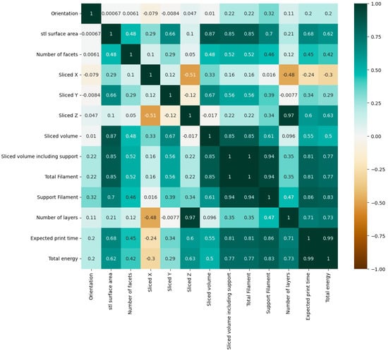
Figure 1. Correlation plot between total energy and other features.

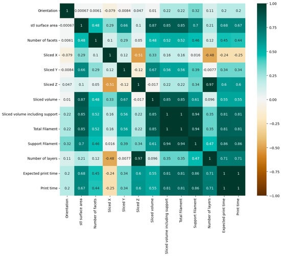
Figure 2. Correlation plot between print time and other features.

In this study, several machine learning algorithms were used to model energy consumption and FDM printing time. These algorithms were chosen not only for their performance and importance in prediction but also for their ability to train data.

5. Methodology

In this section, the algorithms used are briefly introduced, including Multilayer Perceptron (MLP), EXtreme Gradient Boosting (XGBoost), Random Forest (RF) and Support Vector Machines (SVM). These algorithms use data from the experiment cited in article [51] to create each model. Prior to this, several processing operations were carried out on the database to prepare the data for training. This processing mainly concerns the elimination of information that was not relevant to this study (in particular, constant values that had no influence on the modeling result or the appropriateness of values that had to be in a format acceptable to the machine). As a result, 12 inputs in the first column of Table 1 were taken into account in this study. Next, the training to be carried out by each algorithm was based on the distribution applied to the database, with 70% allocated to training data and 30% to test data.

Table 1. The values of the input parameters according to their ranges.

Input Order	Input Parameters FDM	Intervals of Values
INP1	“Orientation” [degree]	0; 90; 180
INP2	“Stl surface area” [mm2]	[1533.85–10,850.92]
INP3	“Number of facets”	[40–9368]
INP4	“Sliced X” [mm]	[3.23–153.87]
INP5	“Sliced Y” [mm]	[8.45–67.27]
INP6	“Sliced Z” [mm]	[3.23–153.87]
INP7	“Sliced volume” [mm3]	[2142.39–5852.08]
INP8	“Sliced volume including support” [mm3]	[2171.28–11,376.59]
INP9	“Total Filament” [g]	[2.76–14.45]
INP10	“Support Filament” [g]	[0–8.13]
INP11	“Expected print time” [h]	[0.4166–4.033]
INP12	“Number of layers” [integer]	[21–1629]

For each algorithm, the best model was chosen by selecting the optimal parameters intrinsic to it (Figure 3). Then, the best approach was chosen by making a statistical comparison of the models selected. These statistical measures concern the MSE, MAE, RMSE, R2 squared and variance explained.

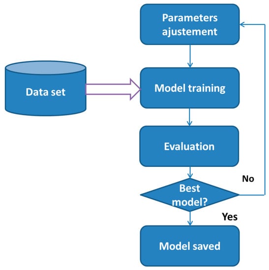
Figure 3. Parameter optimization approach.

5.1. Multilayer Perceptron (MLP)

This type of network belongs to the “feed-forward” class of networks [55,56,57]. The perceptron is increasingly used in many fields of application, such as engineering, medicine, industry and, in particular, additive manufacturing, which has become an increasingly popular technology [23,55,56].

The first mathematical and computer model of the biological neuron was introduced in 1943 by McCulloch and Pitts, who remain the pioneers of modeling and design of neurons [57,58]. Their studies were based on the neuronal properties of the human brain, but they found an analogy between these characteristics and those of computing machines. A multilayer perceptron network is a feed-forward network [59] that consists of three main components: the first element is a layer containing the input features of the network, the second component wraps one or more interconnected hidden layers, and another layer is used for the network output. The constituents of a multilayer perceptron network are the input layer, one or more hidden layers and an output layer with several interconnections that can exist between the neurons of each layer, each interconnection having a synaptic weight carried by a value and the neurons being activated by a differentiable function [60].

The structure of an artificial neuron j is mainly characterized first by a summation function $S_j$ of the signals $X_i\left(i=1,\dots ,m\right)$ of the input layer, weighted by the values of the synaptic weights linked to the connections $w_{ji}\left(i=1,\dots ,m\right)$ according to Equation (1), and second by the activation function $f$, yielding the output value $y_j$.

• The formula for the weighted sum of neuron j is

  $$S_j={\displaystyle \sum _{i=1}^m{w}_{ji}}\times x_i$$

  (1)
• The output $y_j$  is obtained by applying the activation function $f$ according to the following formula:

  $$y_j=f\left({\displaystyle \sum _{i=1}^m(w_{ji}}{x}_i)+b_j\right)$$

  (2)

  $b_j$ refers to the bias of neuron j.

The activation function $f( )$ is a transfer function that can be a “linear function”, “hyperbolic tangent”, “sigmoid”, “radial basis function”, “hyperbolic tangent function” or “ReLU function” [61].

Frequently in a training process, the MLP model uses the backpropagation algorithm to adjust the values of the weights to form the network architecture [60]. The principle of backpropagation is to define an error function and apply gradient descent to calculate the weights that optimize the performance of the model. This training process passes through two essential stages, the forward stage and the backward stage, which are described as follows:

Forward stage: In this stage, the input signal passes through the layers while fixing the values of the synaptic weights until the signal arrives in the output layer [58,62]. The values of the weights are modified by the activation functions and depend closely on the network outputs.

Backward stage: After executing the previous step, an error signal is generated, and then, the required output is compared with the model output. The propagation of this error is directed this time in the opposite direction, and several adjustments are made successively to adapt the values obtained to the weights of the network. This adjustment process is difficult in the hidden layers, but it is simple in the output layer [59,62,63,64].

Backpropagation algorithms are of several types, and the most commonly used are the “Levenberg-Marquardt algorithm”, “gradient descent algorithm”, “scaled conjugate gradient” and “resilient back-propagation one one-step secant algorithm” [58,65,66].

5.2. XGBoost

Chen and Guestrin were the first creators of the XGBoost algorithm [67]. XGBoost is based on tree boosting, an improved machine learning method with a high learning capacity [68]. This algorithm is based on GBDT decision trees with a boosted gradient, and its distinguishing trait is the use of second-order derivatives, unlike conventional decision trees, which only use first-order derivatives. At this stage, XGBoost is more efficient while having a fast calculation, and its formula is expressed by

$$\begin{gathered} {\widehat{y}}_i={\displaystyle \sum _{k=1}^K{f}_k}\left(x_i\right) \\ with: f_k\in F, D={\left\{\left(x_i,y_i\right)\right\}}_{i=1}^n \left(\left|D\right|=n,x_i\in R^m,y_i \in \mathrm{R}\right) \end{gathered}$$

(3)

where ${\widehat{y}}_i$ is the prediction of the sample, $y_i$ is the actual value, $F$ is the whole constituting the K trees, and $f_k\left(x_i\right)$ is the function associated with the k-th tree. The function “objective” of XGBoost is expressed as

$${\mathrm{Obj}}_{}={\displaystyle \sum _{i=1}^{n}l}\left(y_i, {\widehat{y}}_i\right)+{\displaystyle \sum _{i=1}^K\Omega }\left(f_i\right)$$

(4)

where ${\displaystyle \sum _{i=1}^n l}\left(y_i,{\widehat{y}}_i\right)$ is the loss function, allowing us to have the capacity that the prediction model represents. ${\displaystyle \sum _{i=1}^K\Omega }\left(f_i\right)$ is the function with the advantage of regularizing the XGBoost model. The principle of the algorithm is to have a minimized loss function; in other words, the idea of the algorithm is to start from an initial model and to improve it by steps starting from ${\widehat{y}}_i^{ (0)}$ with a null value, which looks like

$$\begin{array}{l}{\widehat{y}}_i^{(1)}=f_1\left(x_i\right)={\widehat{y}}_i^{(0)}+f_1\left(x_i\right)\hfill \\ {\widehat{y}}_i^{(2)}=f_1\left(x_i\right)+f_2\left(x_i\right)={\widehat{y}}_i^{(1)}+f_2\left(x_i\right)\hfill \\ \dots \dots \hfill \\ {\widehat{y}}_i^{(t)}={\displaystyle \sum _{k=1}^t{f}_k}\left(x_i\right)={\widehat{y}}_i^{(t-1)}+f_t\left(x_i\right)\hfill \end{array}$$

(5)

where $f_t(x_i)$ represents the function that gives us the new prediction and ${\widehat{y}}_i^{\left(t-1\right)}$ and ${\widehat{y}}_i^{\left(t\right)}$ represent the respective values of the prediction of the data by the model in iteration (t − 1) and in iteration t. Therefore, the function Obj() can be represented with the following formula:

$$\begin{array}{l}{\mathrm{Obj}}_{}^{\left(t\right)}={\displaystyle \sum _{i=1}^{n}l}\left(y_i,{\widehat{y}}_i^{(t)}\right)+{\displaystyle \sum _{i=1}^t\Omega }\left(f_i\right)=\\ {\displaystyle \sum _{i=1}^{n}l}\left(y_i, {\widehat{y}}_i^{(t-1)}+f_t\left(x_i\right)\right)+{\displaystyle \sum _{i=1}^{t-1^{}}\Omega }\left(f_i\right)+\Omega \left(f_t\right)\end{array}$$

(6)

where $l(y_i,{\widehat{y}}_i^{\left(t-1\right)})$ and ${\widehat{y}}_i^{\left(t-1\right)}$ are two constant values. Then, the Taylor expansion of order 2 is used to obtain an equivalence of the function Obj(). For this, given the two values $h_i={\partial }_{{\widehat{y}}_i^{\left(t-1\right)}}^{2}l(y_i,{\widehat{y}}_i^{\left(t-1\right)})$ and $g_i={\partial }_{{\widehat{y}}_i^{\left(t-1\right)}}l(y_i,{\widehat{y}}_i^{\left(t-1\right)})$, eliminating the contiguous ones, the objective function becomes

$${\mathrm{Obj}}^{\left(t\right)}={\displaystyle \sum }_{i=1}^n\left[(g_i\times f_t\left(x_i\right))+(\frac{1}{2}\times h_i\times f_t^2\left(x_i\right))\right]+ \Omega \left(f_t\right)$$

(7)

With $I_j=\{ i|q(x_i)=j \}$ is the sample on the jth leaf node, and $w_j$ is the weight of the jth node, given that $H_j={\displaystyle \sum _{i\in I_j}}{h}_i$, $G_j={\displaystyle \sum _{i\in I_j}}{g}_i$, and $T$ reflects the number of leaf nodes, the objective function represents:

$${\mathrm{Obj}}^{\left(t\right)}={\displaystyle \sum }_{j=1}^T\left[G_j{w}_j+\frac{1}{2}\left(H_j+\lambda \right)w_j^2\right]+\gamma T$$

(8)

The optimization of the function ${\mathrm{Obj}}^{\left(t\right)}$ gives us

$${\mathrm{Obj}}^{\mathrm{optimal}}=-\frac{1}{2} {\displaystyle \sum }_{j=1}^T \left(\frac{G_j^2}{H_j+\lambda }\right)+\gamma T$$

(9)

The XGBoost algorithm calculates the gain according to the following expression:

$$\mathrm{Gain}=\frac{1}{2}\times \left[(\frac{G_R^2}{H_R+\lambda })+(\frac{G_L^2}{H_L+\lambda })-(\frac{{\left(G_L+G_R\right)}^2}{H_L+H_R+\lambda })\right]-\gamma$$

(10)

where $(\frac{G_R^2}{H_R+\lambda })$, $(\frac{G_L^2}{H_L+\lambda })$ and $(\frac{{\left(G_L+G_R\right)}^2}{H_L+H_R+\lambda })$ correspond to the scores of the right and left subtrees and of the node that is not split, respectively.

5.3. Random Forest Regression

This type of algorithm is a combination of statistical learning theory and decision trees. It was first introduced by Breiman (2001) [69]. The RF algorithm has been widely used in regression because of the precision it brings in terms of performance. Random Forest uses decision trees, and an original bootstrap sample of data is associated with each tree. The vote prediction is calculated based on the calculated predictions of each tree. In other words, the algorithm aims to determine the regression result while combining the decision trees that are weak in a strong tree with more precision. RFR has several advantages compared to other algorithms, including that it is stable and that there is no overfitting problem [70]. In addition, this algorithm does not require several configuration parameters and is easy to use. The formula for the RFR regression predictor is:

$${\widehat{F}}_{rf}^K(x)=\frac{1}{k}\times {\displaystyle \sum _{u=1}^K{T}_u^{}}(x)$$

(11)

where k is the number of decision trees and $T_u^{}$ is the prediction of the u th decision tree.

5.4. Support Vector Machines (SVM)

On a training space $X$ of size N, where $X\in R^n,$ let $\left(x_1,y_1\right),\dots ,\left(x_N,y_N\right)$ be input elements, with $x_i\in X,y_i\in R$. The desired objective is to find an SVM function for the regression of the data, whose mathematical form usually takes the form of the following equation [71,72]:

$$f(x)=(w\times \phi (x))+b$$

(12)

$\varphi :X\to \Omega$ is a function whose output is the feature space, and $b\in R$.

The objective is to find $w$ and $b$ while minimizing the following function:

$$R(f)=C{\displaystyle \sum _{j=1}^N\Gamma }\left(f\left(x_j\right)-y_j\right)+\frac{1}{2}(w\times w)$$

(13)

$$\Gamma (f(x)-y)=\left\{ \begin{array}{cc}0,& \mathrm{if} \mathrm{val}<\epsilon \\ \mathrm{val}-\epsilon ,& \mathrm{otherwise} \end{array}\right.$$

(14)

where $C$ is a predefined value, $\Gamma$ is the cost function measuring the empirical risk, $\epsilon$ is a cost-insensitive function and $\mathrm{val}=|y-f(x\left)\right|$.

6. Model Comparison and Validation

In this study, the MLP, XGBoost, RF Regressor and SVM Regressor algorithms were used to build predictive models of energy consumption and time used in the FDM process, based on the dataset cited in Table 1 and following the methodology described in the Section 5. A statistical comparison of the algorithms used, based on the five performance criteria (MAE, MSE, RMSE, R2 squared and variance explained), clearly shows that the MLP-based model has higher performance measures than the other models. The following table illustrates the statistical values obtained:

Figure 4 and Figure 5 illustrate the relative representations of the energy consumption and printing time of the models used. The neural algorithm developed corresponds well to the experimental values, which is also justified by the statistical performance values.

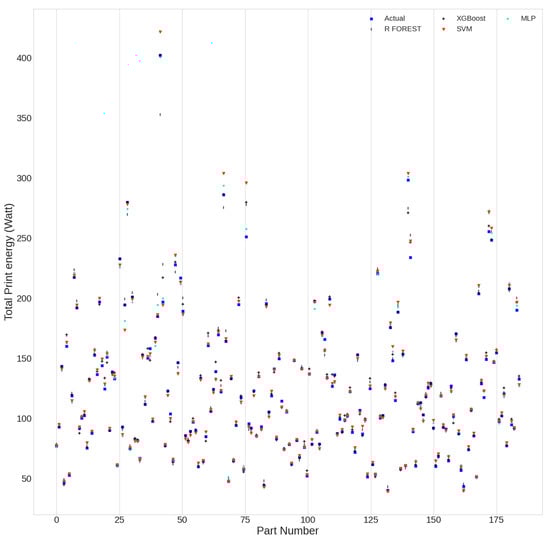
Figure 4. Actual and predicted energy values for each part.

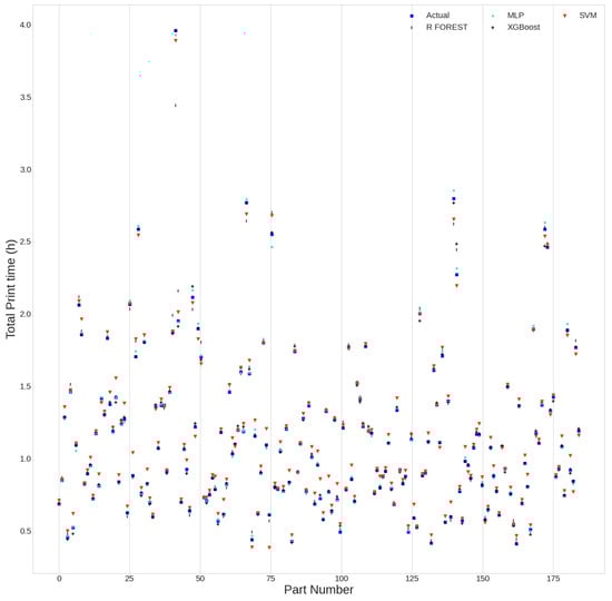
Figure 5. Actual and predicted print time values for each part.

From the statistical measurements recorded in Table 2 and the representations of the two figures of energy consumption and FDM printing time, it is clear that the proposed neural model outperforms the other models. In these figures, it can be seen that the experimental values for 184 parts (x-axis) and the predicted values of the proposed model (y-axis) are closer together than in the other models. In the following section, details of the strategy followed to obtain the adopted model will be presented.

Table 2. Performance of the used models.

Model.	MAE	MSE	RMSE	R-Squared	Explained Variance
XGBoost	2.57167085	31.7460321	5.63436173	98.4415807	98.4661312
Random Forest	2.46675634	35.1311636	5.92715476	97.9773199	97.9841714
Support Vector Regression	1.42252208	7.39417652	2.71922351	99.0687064	99.0862437
Proposed model (MLP)	0.989	0.018	1.355	99.59	99.6

7. Adopted Model

In the case of this study, there are twelve inputs and two outputs, so automatically, the input layer must have twelve neurons, and two neurons must be assigned to the output layer. To prove the structure of the hidden layers, 156 networks were developed with the following architectures using the Keras library:

One hidden layer: 12-i-2, such as 2 ≤ i ≤ 13.

Two hidden layers: 12-i-j-2, such as 2 ≤ i,j ≤ 13.

For each architecture, to find the best model, different activation functions were used, such as exponential, elu, selu, tanh, softsing, softplus, softmax, sigmoid and ReLU.

As a first step, before proceeding with the training of each architecture, the dataset was divided into two parts, 30% for testing and 70% for training, and then normalized using the MinMaxScaler function.

Five performance criteria were calculated for each architecture: R2 Square, Ex-plained-Variance, MAE, MSE and RMSE. According to the results, using the sigmoid activation function to activate the hidden layers and activating the output layer using the ReLU function yielded good performance; however, using the other activation functions yielded less accuracy. Table 3 shows some of the architectures that performed well.

Table 3. Performance of the selected networks.

MLP Network	R2 Square	Explained-Variance	MAE	MSE	RMSE
12-2-2	99.34%	99.56%	1.248%	0.03%	1.72%
12-6-2	97.55%	97.73%	2.004%	0.11%	3.314%
12-8-2	97.81%	97.95%	1.88%	0.098%	3.131%
12-12-2	97.94%	98.11%	1.908%	0.092%	3.036%
12-2-4-2	99.59%	99.6%	0.989%	0.018%	1.355%
12-2-11-2	99.4%	99.44%	1.133%	0.027%	1.638%
12-2-12-2	98.83%	98.84%	1.377%	0.052%	2.289%
12-3-2-2	99.51%	99.51%	0.973%	0.022%	1.479%
12-3-6-2	98.25%	98.25%	1.466%	0.079%	2.802%
12-3-8-2	96.96%	96.99%	1.595%	0.136%	3.691%
12-4-4-2	97.21%	97.41%	1.765%	0.125%	3.535%
12-6-13-2	98.25%	98.38%	1.887%	0.078%	2.801%
12-9-6-2	98.17%	98.3%	1.706%	0.082%	2.864%

According to the results reported in Table 3, the optimal architecture corresponds to two hidden layers. The first two hidden layers are activated by the sigmoid function, and they have four neurons and two neurons. The output layer is activated by the ReLU function, and two neurons are used in this layer (Figure 6). This architecture provides the following performance: R2 = 99.59%, explained variance = 99.60%, MAE = 0.989%, MSE = 0.018% and RMSE = 1.355%.

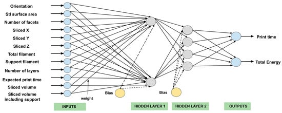
Figure 6. MLP architecture of the selected network.

At epoch 1523, successful training was achieved with an MSE value equal to 0.018% (Figure 7). The weights and biases of the optimized model are shown in Table 4, Table 5 and Table 6.

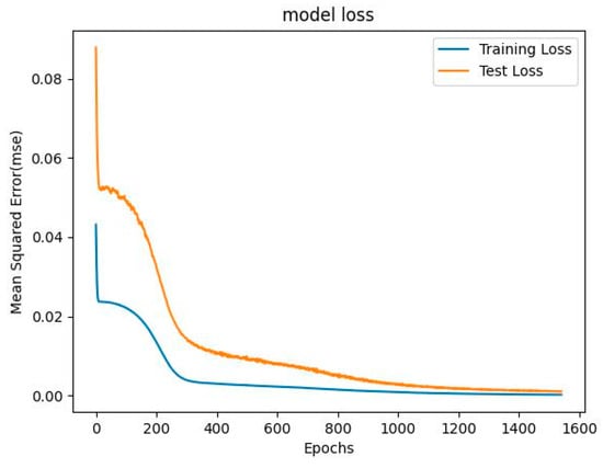
Figure 7. MSE variations vs. epoch during training of the optimal network.

Table 4. Weights and biases for the first hidden layer.

		Neurons of First Hidden Layer
		1	2
Neurons of input layer	1	−0.01860396	0.01651467
	2	−0.39869556	0.02904175
	3	0.06080785	−0.15600291
	4	0.00827086	−0.07250348
	5	−0.08958101	0.08917017
	6	0.24706206	−0.14367856
	7	0.0626247	0.09804111
	8	0.0649894	0.09762235
	9	−0.02316719	0.12844889
	10	−0.12178944	−0.03211394
	11	4.598817	2.9437175
	12	0.01480456	0.01575648
	biases	−0.42479023	−3.8425364

Table 5. Weights and bias of the second hidden layer.

		Neurons of Second Hidden Layer
		1	2	3	4
Neurons of first hidden layer	1	1.7487305	1.1139799	−0.8182974	1.1671507
	2	0.9893758	2.1798441	−2.780944	7.2701535
	biases	−0.72620803	−1.2299542	1.136458	−0.7672453

Table 6. Weights and biases for the output layer.

		Neurons of Output Layer
		1	2
Neurons of second hidden layer	1	0.13126287	1.0074766
	2	0.21024154	0.90955585
	3	−0.7737203	−1.1061413
	4	1.271458	0.0429178
	biases	−0.1821677	−0.05179993

To demonstrate the effectiveness of the model obtained, the predicted values and the experimental values are compared in Figure 8 and Figure 9, thus representing the trend between the actual values and those given by the proposed model according to energy consumption and FDM printing time.

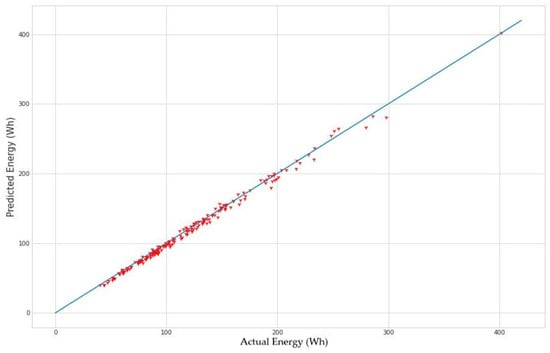
Figure 8. Trend line of actual and predicted values for energy consumption.

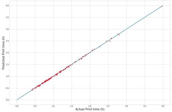
Figure 9. Trend line of actual and predicted values for print time.

8. Discussion

The current investigation aims to simultaneously predict energy consumption and printing time by providing the correct orientation that optimizes both costs. To validate this model, Figure 10 and Figure 11 illustrate the trends in experimental values compared with the predicted values of the proposed model. Thus, the “part number” designating the parts according to their order in the database are shown on the x-axis, while the predicted values (energy in Figure 10 and printing time in Figure 11) are marked on the y-axis.

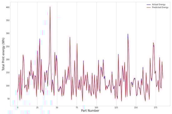
Figure 10. Actual and predicted values of energy for the 184 experiments.

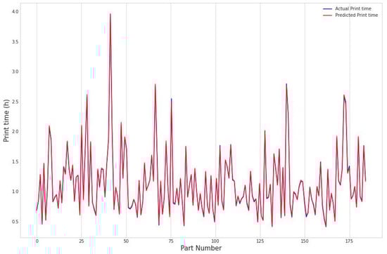
Figure 11. Actual and predicted values of the printing time for 184 experiments.

According to both representations, there is harmony between the experimental and predicted values. Moreover, both curves behave in a similar way to the actual values, which is justified by the quasi-juxtaposition of each curve with the experimental values. The result clearly shows the effectiveness of the proposed model.

From the dataset [25], four parts were randomly selected to evaluate the effectiveness of the proposed approach. Table 7 shows the experimental and predicted values of FDM printing energy and time for each of the four parts.

Table 7. Some use cases, with comparison between the two real and predicted values.

Part	Orientation (Degree)	Predicted Energy (Watt)	Actual Energy (Watt)	Error of Prediction (Energy)	Predicted Print Time (Hour)	Actual Print Time (Hour)	Error of Prediction (Print Time)
	0	150.23254	143.864	0.04426778	1.3921772	1.375	0.01249251
	90	127.927956	124.446	0.02797965	1.187228	1.188	0.00064983
	180	154.8057	150.982	0.02532554	1.441631	1.423	0.01309276
	0	150.10175	152.63	0.01656457	1.3728974	1.36	0.00948338
	90	117.2996	111.817	0.0490319	1.089192	1.071	0.01698599
	180	151.03885	150.167	0.00580587	1.3892009	1.367	0.0162406
	0	124.42141	122.171	0.01842017	1.1680287	1.186	0.01515287
	90	282.67624	285.951	0.01145217	2.7901657	2.767	0.00837214
	180	170.33725	164.24	0.03712403	1.6079372	1.587	0.01319294
	0	95.08733	97.391	0.02365383	0.8763252	0.873	0.00380893
	90	102.01913	102.175	0.00152552	0.9368667	0.93	0.00738355
	180	118.05182	120.406	0.01955202	1.0821551	1.084	0.00170194

This test takes into account the three orientations (0, 90 and 180) and then calculates the prediction error for each orientation (15):

$$\mathrm{Error} \mathrm{of} \mathrm{prediction}=\frac{\mid \mathrm{Predict} \mathrm{value} - \mathrm{Experimental} \mathrm{value} \mid }{ \mathrm{Experimental} \mathrm{value} }$$

(15)

• Part 1 must be printed in direction 90; if printing is done in another direction, a loss of 0 h 20 min in terms of time and 25 Watt in terms of energy will occur.
• Part 2 should be printed in direction 90; if printing is done in another direction, a loss of 0 h 20 min in terms of time and 40 Watt in terms of energy will occur.
• Part 3 should be printed in direction 0; if printing is done in another direction, a loss of 1 h 30 min in terms of time and 250 Watt in terms of energy will occur.
• Part 4 should be printed in direction 0; if printing is done in another direction, a loss of 0 h 15 min in terms of time and 23 Watt in terms of energy will occur.

On the basis of the results presented in Table 7, it is clear that the proposed model can be used effectively to select the correct part orientation, while energy consumption and printing time can be achieved at optimum cost.

9. Conclusions

In this research, a model was proposed to predict energy consumption and FDM printing time based on experience extracted from [25]. In this sense, four machine learning algorithms were used, given their performance in prediction and training. A comparative study was carried out, clearly showing that the proposed neural network model performed significantly better than the other models used. Calculation of the model’s overall performance yielded the following statistical values: 0.018% for the MSE value, 99.60% for the explained variance value, 0.989% for the MAE value, 99.59% for the R-squared value and 1.355% for the RMSE value.

Using this model, the energy consumption and printing time for different part orientations were estimated efficiently. In addition, the proposed approach offers the possibility of choosing the optimal orientation that minimizes both the energy and time costs in FDM printing.

This study remains useful for understanding the energy and time consumption of 3D manufacturing, which could provide a decision support tool for practicians to improve energy and time inefficiency factors. This can be extended to other computer-aided manufacturing processes that could benefit from the applicability of the current research results.

For future work, a study of additive manufacturing is envisaged to predict and optimize other resources related to the manufacture of 3D-printed parts, taking into account the effect of other parameters that influence this process. In addition, this paper could provide a basis for studying the energy consumption and print time of parts manufactured in 4D, while taking advantage of the benefits provided by this technology. Finally, this work will represent a benchmark that could be improved by taking into account the environmental aspect while studying possible disciplines related to additive manufacturing.

References

- Wohlers Report 2023–Wohlers Associates. Available online: https://wohlersassociates.com/product/wr2023/ (accessed on 16 June 2023).
- Han, Q.; Setchi, R.; Evans, S.L. Synthesis and characterisation of advanced ball-milled Al-Al2O3 nanocomposites for selective laser melting. Powder Technol. 2016, 297, 183–192. [Google Scholar] [CrossRef]
- Huang, R.; Riddle, M.; Graziano, D.; Warren, J.; Das, S.; Nimbalkar, S.; Cresko, J.; Masanet, E. Energy and emissions saving potential of additive manufacturing: The case of lightweight aircraft components. J. Clean. Prod. 2016, 135, 1559–1570. [Google Scholar] [CrossRef]
- Arifin, N.A.M.; Saman, M.Z.M.; Sharif, S.; Ngadiman, N.H.A. Sustainability Implications of Additive Manufacturing. In Human-Centered Technology for a Better Tomorrow; Hassan, M.H.A., Ahmad Manap, Z., Baharom, M.Z., Johari, N.H., Jamaludin, U.K., Jalil, M.H., Mat Sahat, I., Omar, M.N., Eds.; Lecture Notes in Mechanical Engineering; Springer: Singapore, 2022; pp. 441–452. ISBN 9789811641145. [Google Scholar]
- Vidakis, N.; Kechagias, J.D.; Petousis, M.; Vakouftsi, F.; Mountakis, N. The effects of FFF 3D printing parameters on energy consumption. Mater. Manuf. Process. 2023, 38, 915–932. [Google Scholar] [CrossRef]
- Chaudhary, R.; Fabbri, P.; Leoni, E.; Mazzanti, F.; Akbari, R.; Antonini, C. Additive manufacturing by digital light processing: A review. Prog. Addit. Manuf. 2023, 8, 331–351. [Google Scholar] [CrossRef]
- F42 Committee. Terminology for Additive Manufacturing Technologies; ASTM International: West Conshohocken, PA, USA, 2013. [Google Scholar]
- Kellens, K.; Baumers, M.; Gutowski, T.G.; Flanagan, W.; Lifset, R.; Duflou, J.R. Environmental Dimensions of Additive Manufacturing: Mapping Application Domains and Their Environmental Implications. J. Ind. Ecol. 2017, 21, S49–S68. [Google Scholar] [CrossRef]
- ISO/ASTM 52900:2021; Additive Manufacturing—General Principles—Fundamentals and Vocabulary. Available online: https://www.iso.org/standard/74514.html (accessed on 1 July 2023).
- Gibson, I.; Rosen, D.; Stucker, B.; Khorasani, M. Additive Manufacturing Technologies; Springer International Publishing: Berlin/Heidelberg, Germany, 2021; ISBN 978-3-030-56126-0. [Google Scholar]
- Godec, D.; Pilipović, A.; Breški, T.; Ureña, J.; Jordá, O.; Martínez, M.; Gonzalez-Gutierrez, J.; Schuschnigg, S.; Blasco, J.R.; Portolés, L. Introduction to Additive Manufacturing. In A Guide to Additive Manufacturing; Godec, D., Gonzalez-Gutierrez, J., Nordin, A., Pei, E., Ureña Alcázar, J., Eds.; Springer Tracts in Additive Manufacturing; Springer International Publishing: Berlin/Heidelberg, Germany, 2022; pp. 1–44. ISBN 978-3-031-05862-2. [Google Scholar]
- Verhoef, L.A.; Budde, B.W.; Chockalingam, C.; García Nodar, B.; Van Wijk, A.J.M. The effect of additive manufacturing on global energy demand: An assessment using a bottom-up approach. Energy Policy 2018, 112, 349–360. [Google Scholar] [CrossRef]
- Song, R.; Telenko, C. Material and energy loss due to human and machine error in commercial FDM printers. J. Clean. Prod. 2017, 148, 895–904. [Google Scholar] [CrossRef]
- Lalegani Dezaki, M.; Mohd Ariffin, M.K.A.; Hatami, S. An overview of fused deposition modelling (FDM): Research, development and process optimisation. Rapid Prototyp. J. 2021, 27, 562–582. [Google Scholar] [CrossRef]
- Hegab, H.; Khanna, N.; Monib, N.; Salem, A. Design for sustainable additive manufacturing: A review. Sustain. Mater. Technol. 2023, 35, e00576. [Google Scholar] [CrossRef]
- Yoon, H.-S.; Lee, J.-Y.; Kim, H.-S.; Kim, M.-S.; Kim, E.-S.; Shin, Y.-J.; Chu, W.-S.; Ahn, S.-H. A comparison of energy consumption in bulk forming, subtractive, and additive processes: Review and case study. Int. J. Precis. Eng. Manuf.-Green Technol. 2014, 1, 261–279. [Google Scholar] [CrossRef]
- Rejeski, D.; Zhao, F.; Huang, Y. Research Needs and Recommendations on Environmental Implications of Additive Manufacturing. Addit. Manuf. 2017, 19, 21–28. [Google Scholar] [CrossRef]
- Hopkins, N.; Jiang, L.; Brooks, H. Energy consumption of common desktop additive manufacturing technologies. Clean. Eng. Technol. 2021, 2, 100068. [Google Scholar] [CrossRef]
- Ajay, J.; Song, C.; Rathore, A.S.; Zhou, C.; Xu, W. 3DGates: An Instruction-Level Energy Analysis and Optimization of 3D Printers. In Proceedings of the Twenty-Second International Conference on Architectural Support for Programming Languages and Operating Systems, Xi’an, China, 4 April 2017; pp. 419–433. [Google Scholar]
- Weissman, A.; Gupta, S.K. Selecting a Design-Stage Energy Estimation Approach for Manufacturing Processes. In Proceedings of the 23rd International Conference on Design Theory and Methodology, Washington, DC, USA, 28–31 August 2011; Volume 9, pp. 1075–1086. [Google Scholar]
- Tian, X.; Wu, L.; Gu, D.; Yuan, S.; Zhao, Y.; Li, X.; Ouyang, L.; Song, B.; Gao, T.; He, J.; et al. Roadmap for Additive Manufacturing: Toward Intellectualization and Industrialization. Chin. J. Mech. Eng. Addit. Manuf. Front. 2022, 1, 100014. [Google Scholar] [CrossRef]
- Qin, J.; Liu, Y.; Grosvenor, R. Multi-source data analytics for AM energy consumption prediction. Adv. Eng. Inform. 2018, 38, 840–850. [Google Scholar] [CrossRef]
- Yang, Y.; He, M.; Li, L. Power consumption estimation for mask image projection stereolithography additive manufacturing using machine learning based approach. J. Clean. Prod. 2020, 251, 119710. [Google Scholar] [CrossRef]
- Jia, S.; Yuan, Q.; Cai, W.; Li, M.; Li, Z. Energy modeling method of machine-operator system for sustainable machining. Energy Convers. Manag. 2018, 172, 265–276. [Google Scholar] [CrossRef]
- r3DiM Benchmark. Available online: https://www.kaggle.com/dataset/c22f9996866156344599fd5baf48aaa8ac8ccce9a849b050ceeea36ba4e9c8f9 (accessed on 25 June 2022).
- Rahmatabadi, D.; Aberoumand, M.; Soltanmohammadi, K.; Soleyman, E.; Ghasemi, I.; Baniassadi, M.; Abrinia, K.; Bodaghi, M.; Baghani, M. 4D Printing-Encapsulated Polycaprolactone–Thermoplastic Polyurethane with High Shape Memory Performances. Adv. Eng. Mater. 2023, 25, 2201309. [Google Scholar] [CrossRef]
- Rahmatabadi, D.; Aberoumand, M.; Soltanmohammadi, K.; Soleyman, E.; Ghasemi, I.; Baniassadi, M.; Abrinia, K.; Zolfagharian, A.; Bodaghi, M.; Baghani, M. A New Strategy for Achieving Shape Memory Effects in 4D Printed Two-Layer Composite Structures. Polymers 2022, 14, 5446. [Google Scholar] [CrossRef]
- Aberoumand, M.; Soltanmohammadi, K.; Soleyman, E.; Rahmatabadi, D.; Ghasemi, I.; Baniassadi, M.; Abrinia, K.; Baghani, M. A comprehensive experimental investigation on 4D printing of PET-G under bending. J. Mater. Res. Technol. 2022, 18, 2552–2569. [Google Scholar] [CrossRef]
- Monzón, M.D.; Paz, R.; Pei, E.; Ortega, F.; Suárez, L.A.; Ortega, Z.; Alemán, M.E.; Plucinski, T.; Clow, N. 4D printing: Processability and measurement of recovery force in shape memory polymers. Int. J. Adv. Manuf. Technol. 2017, 89, 1827–1836. [Google Scholar] [CrossRef]
- Bodaghi, M.; Damanpack, A.R.; Liao, W.H. Adaptive metamaterials by functionally graded 4D printing. Mater. Des. 2017, 135, 26–36. [Google Scholar] [CrossRef]
- Cerbe, F.; Sinapius, M.; Böl, M. Methodology for FDM 4D printing with thermo-responsive SMPs. Mater. Today Proc. 2022, in press. [Google Scholar] [CrossRef]
- Peng, T. Analysis of Energy Utilization in 3D Printing Processes. Procedia CIRP 2016, 40, 62–67. [Google Scholar] [CrossRef]
- Quantifying the Overall Impact of Additive Manufacturing on Energy Demand: The Case of Selective Laser-Sintering Processes for Automotive and Aircraft Components. Available online: https://www.eceee.org/library/conference_proceedings/eceee_Industrial_Summer_Study/2016/2-sustainable-production-design-and-supply-chain-initiatives/quantifying-the-overall-impact-of-additive-manufacturing-on-energy-demand-the-case-of-selective-laser-sintering-processes-for-automotive-and-aircraft-components/ (accessed on 8 August 2022).
- Yan, Z.; Huang, J.; Lv, J.; Hui, J.; Liu, Y.; Zhang, H.; Yin, E.; Liu, Q. A New Method of Predicting the Energy Consumption of Additive Manufacturing considering the Component Working State. Sustainability 2022, 14, 3757. [Google Scholar] [CrossRef]
- Harding, O.J.; Griffiths, C.A.; Rees, A.; Pletsas, D. Methods to Reduce Energy and Polymer Consumption for Fused Filament Fabrication 3D Printing. Polymers 2023, 15, 1874. [Google Scholar] [CrossRef]
- Yang, J.; Liu, Y. Energy, time and material consumption modelling for fused deposition modelling process. Procedia CIRP 2020, 90, 510–515. [Google Scholar] [CrossRef]
- Petousis, M.; Vidakis, N.; Mountakis, N.; Karapidakis, E.; Moutsopoulou, A. Compressive response versus power consumption of acrylonitrile butadiene styrene in material extrusion additive manufacturing: The impact of seven critical control parameters. Int. J. Adv. Manuf. Technol. 2023, 126, 1233–1245. [Google Scholar] [CrossRef]
- Monteiro, H.; Carmona-Aparicio, G.; Lei, I.; Despeisse, M. Energy and material efficiency strategies enabled by metal additive manufacturing–A review for the aeronautic and aerospace sectors. Energy Rep. 2022, 8, 298–305. [Google Scholar] [CrossRef]
- Baumers, M.; Tuck, C.; Wildman, R.; Ashcroft, I.; Rosamond, E.; Hague, R. Transparency Built-in. J. Ind. Ecol. 2013, 17, 418–431. [Google Scholar] [CrossRef]
- Meteyer, S.; Xu, X.; Perry, N.; Zhao, Y.F. Energy and Material Flow Analysis of Binder-jetting Additive Manufacturing Processes. Procedia CIRP 2014, 15, 19–25. [Google Scholar] [CrossRef]
- Verma, A.; Rai, R.; Lab, D. Energy Efficient Modeling and Optimization of Additive Manufacturing Processes. In Proceedings of the 24th International SFF Symposium—An Additive Manufacturing Conference, SFF, Austin, TX, USA, 12–14 August 2013; Available online: https://hdl.handle.net/2152/88493 (accessed on 25 June 2022).
- Yang, Y.; Li, L.; Pan, Y.; Sun, Z. Energy Consumption Modeling of Stereolithography-Based Additive Manufacturing Toward Environmental Sustainability. J. Ind. Ecol. 2017, 21, S168–S178. [Google Scholar] [CrossRef]
- Simon, T.R.; Lee, W.J.; Spurgeon, B.E.; Boor, B.E.; Zhao, F. An Experimental Study on the Energy Consumption and Emission Profile of Fused Deposition Modeling Process. Procedia Manuf. 2018, 26, 920–928. [Google Scholar] [CrossRef]
- Luo, Y.; Leu, M.C.; Ji, Z. Assessment of Environmental Performance of Rapid Prototyping and Rapid Tooling Processes. In Proceedings of the 10th Annual Solid Freeform Fabrication Symposium, Austin, TX, USA, 9–11 August 1999; pp. 783–791. [Google Scholar]
- Jackson, M.; Asten, A.; Morrow, J.; Min, S.; Pfefferkorn, F. Comparison of Energy Consumption in Wire-based and Powder-based Additive-subtractive Manufacturing. Procedia Manuf. 2016, 5, 989–1005. [Google Scholar] [CrossRef]
- Qin, J.; Hu, F.; Liu, Y.; Witherell, P.; Wang, C.C.L.; Rosen, D.W.; Simpson, T.W.; Lu, Y.; Tang, Q. Research and application of machine learning for additive manufacturing. Addit. Manuf. 2022, 52, 102691. [Google Scholar] [CrossRef]
- Kumar, R.; Ghosh, R.; Malik, R.; Sangwan, K.S.; Herrmann, C. Development of Machine Learning Algorithm for Characterization and Estimation of Energy Consumption of Various Stages during 3D Printing. Procedia CIRP 2022, 107, 65–70. [Google Scholar] [CrossRef]
- Hu, F.; Qin, J.; Li, Y.; Liu, Y.; Sun, X. Deep Fusion for Energy Consumption Prediction in Additive Manufacturing. Procedia CIRP 2021, 104, 1878–1883. [Google Scholar] [CrossRef]
- McComb, C.; Meisel, N.; Simpson, T.W.; Murphy, C. Predicting Part Mass, Required Support Material, and Build Time via Autoencoded Voxel Patterns; Pennsylvania State University: State College, PA, USA, 2018; Available online: https://engrxiv.org/preprint/view/247 (accessed on 25 June 2022). [CrossRef]
- El youbi El idrissi, M.A.; Laaouina, L.; Jeghal, A.; Tairi, H.; Zaki, M. Energy Consumption Prediction for Fused Deposition Modelling 3D Printing Using Machine Learning. Appl. Syst. Innov. 2022, 5, 86. [Google Scholar] [CrossRef]
- Szemeti, G.; Ramanujan, D. An Empirical Benchmark for Resource Use in Fused Deposition Modelling 3D Printing of Isovolumetric Mechanical Components. Procedia CIRP 2022, 105, 183–191. [Google Scholar] [CrossRef]
- Durgashyam, K.; Indra Reddy, M.; Balakrishna, A.; Satyanarayana, K. Experimental investigation on mechanical properties of PETG material processed by fused deposition modeling method. Mater. Today Proc. 2019, 18, 2052–2059. [Google Scholar] [CrossRef]
- Guessasma, S.; Belhabib, S.; Nouri, H. Printability and Tensile Performance of 3D Printed Polyethylene Terephthalate Glycol Using Fused Deposition Modelling. Polymers 2019, 11, 1220. [Google Scholar] [CrossRef]
- Pernica, J.; Sustr, M.; Dostal, P.; Brabec, M.; Dobrocky, D. Tensile Testing of 3D Printed Materials Made by Different Temperature. Manuf. Technol. 2021, 21, 398–404. [Google Scholar] [CrossRef]
- Qi, X.; Chen, G.; Li, Y.; Cheng, X.; Li, C. Applying Neural-Network-Based Machine Learning to Additive Manufacturing: Current Applications, Challenges, and Future Perspectives. Engineering 2019, 5, 721–729. [Google Scholar] [CrossRef]
- Kwon, O.; Kim, H.G.; Ham, M.J.; Kim, W.; Kim, G.-H.; Cho, J.-H.; Kim, N.I.; Kim, K. A deep neural network for classification of melt-pool images in metal additive manufacturing. J. Intell. Manuf. 2020, 31, 375–386. [Google Scholar] [CrossRef]
- Dreyfus, G.; Martinez, J.-M.; Samuelides, M.; Gordon, M.B.; Badran, F.; Thiria, S.; Hérault, L. Réseaux de Neurones. Librairie Eyrolles. Available online: https://www.eyrolles.com/Informatique/Livre/reseaux-de-neurones-9782212110197 (accessed on 25 June 2022).
- McCulloch, W.S.; Pitts, W. A logical calculus of the ideas immanent in nervous activity. Bull. Math. Biophys. 1943, 5, 115–133. [Google Scholar] [CrossRef]
- Huang, Y. Advances in Artificial Neural Networks–Methodological Development and Application. Algorithms 2009, 2, 973–1007. [Google Scholar] [CrossRef]
- Haykin, S.S. Neural Networks and Learning Machines; Pearson International Edition; Pearson: London, UK, 2009; Available online: https://books.google.co.ma/books?id=KCwWOAAACAAJ (accessed on 25 June 2022).
- Ramachandran, P.; Zoph, B.; Le, Q.V. Searching for Activation Functions. arXiv 2017, arXiv:1710.05941. [Google Scholar]
- Rosenblatt, F. Perceptron Simulation Experiments. Proc. IRE 1960, 48, 301–309. [Google Scholar] [CrossRef]
- Chauvin, Y.; Rumelhart, D.E. (Eds.) Backpropagation: Theory, Architectures, and Applications; Lawrence Erlbaum Associates, Inc.: Hillsdale, NJ, USA, 1995; p. 561. ISBN 978-0-8058-1258-9. [Google Scholar]
- Hopfield, J.J. Neural networks and physical systems with emergent collective computational abilities. Proc. Natl. Acad. Sci. USA 1982, 79, 2554–2558. [Google Scholar] [CrossRef]
- Haykin, S.S.; Haykin, S.S. Neural Networks and Learning Machines, 3rd ed.; Prentice Hall: New York, NY, USA, 2009; ISBN 978-0-13-147139-9. [Google Scholar]
- Corriou, J.-P.; Société de Chimie Industrielle; Société Française de Génie des Procédés. Journée D’étude Modélisation, Conduite et Diagnostic de Procédés Industriels à l’aide de Réseaux de Neurones; Organisée Conjointement par le GFGP et la Société de Chimie Industrielle, 29 Mars 1995; Coordonnateur Jean Pierre Corriou; Lavoisier Technique et Documentation: Paris, France, 1995; ISBN 2-910239-11-X. [Google Scholar]
- Chen, T.; Guestrin, C. XGBoost: A Scalable Tree Boosting System. In Proceedings of the 22nd ACM SIGKDD International Conference on Knowledge Discovery and Data Mining, San Francisco, CA, USA, 13 August 2016; pp. 785–794. [Google Scholar] [CrossRef]
- Zhang, Z.; Zhang, Y.; Wen, Y.; Ren, Y. Data-driven XGBoost model for maximum stress prediction of additive manufactured lattice structures. Complex Intell. Syst. 2023, 1–12. [Google Scholar] [CrossRef]
- Breiman, L. Random Forests. Mach. Learn. 2001, 45, 5–32. [Google Scholar] [CrossRef]
- Liu, D.; Fan, Z.; Fu, Q.; Li, M.; Faiz, M.A.; Ali, S.; Li, T.; Zhang, L.; Khan, M.I. Random forest regression evaluation model of regional flood disaster resilience based on the whale optimization algorithm. J. Clean. Prod. 2020, 250, 119468. [Google Scholar] [CrossRef]
- Smola, A.J.; Schölkopf, B. A tutorial on support vector regression. Stat. Comput. 2004, 14, 199–222. [Google Scholar] [CrossRef]
- Vapnik, V.N. The Nature of Statistical Learning Theory; Springer: New York, NY, USA, 1995; ISBN 978-1-4757-2440-0. [Google Scholar]
Disclaimer/Publisher’s Note: The statements, opinions and data contained in all publications are solely those of the individual author(s) and contributor(s) and not of MDPI and/or the editor(s). MDPI and/or the editor(s) disclaim responsibility for any injury to people or property resulting from any ideas, methods, instructions or products referred to in the content. |
© 2023 by the authors. Licensee MDPI, Basel, Switzerland. This article is an open access article distributed under the terms and conditions of the Creative Commons Attribution (CC BY) license (https://creativecommons.org/licenses/by/4.0/).