Integration of Deep Sequence Learning-Based Virtual GPS Model and EKF for AUV Navigation

Abstract

To address the issue of increasing navigation errors in low-cost autonomous underwater vehicles (AUVs) operating without assisted positioning underwater, this paper proposes a Virtual GPS Model (VGPSM) based on deep sequence learning. This model is integrated with an Extended Kalman Filter (EKF) to provide a high-precision navigation solution for AUVs. The VGPSM leverages the time-series characteristics of data from sensors such as the Attitude and Heading Reference System (AHRS) and the Doppler Velocity Log (DVL) while the AUV is on the surface. It learns the relationship between these sensor data and GPS data by utilizing a hybrid model of Long Short-Term Memory (LSTM) and Bidirectional Long Short-Term Memory (Bi-LSTM), which are well-suited for processing and predicting time-series data. This approach constructs a virtual GPS model that generates virtual GPS displacements updated at the same frequency as the real GPS data. When the AUV navigates underwater, the virtual GPS displacements generated using the VGPSM in real-time are used as measurements to assist the EKF in state estimation, thereby enhancing the accuracy and robustness of underwater navigation. The effectiveness of the proposed method is validated through a series of experiments under various conditions. The experimental results demonstrate that the proposed method significantly reduces cumulative errors, with navigation accuracy improvements ranging from 29.2% to 69.56% compared to the standard EKF, indicating strong adaptability and robustness.

1. Introduction

With the rapid development of marine science and technology, the demand for autonomous underwater vehicles (AUVs) in civil, military, and scientific research fields is increasing [1]. As the core component of AUV autonomy and intelligence, the positioning accuracy of the navigation system directly affects the success and efficiency of AUV underwater missions [2,3]. However, the special characteristics of the underwater environment bring great challenges to the navigation and positioning of AUVs [4,5]. Therefore, it is of great research significance to improve the navigation accuracy of underwater vehicles.

Currently, AUV underwater navigation sensors mainly include the inertial navigation system (INS) [6], Doppler Velocimetry (DVL) [7], a Depth System (PS) [8], and a Global Positioning System (GPS) [9]. In general, INS can provide AUVs with acceleration, angular velocity, angle, velocity, and position information. However, since the calculation of velocity and position relies on the integral accumulation of acceleration and angular velocity, it requires the high accuracy of gyroscopes and accelerometers. Conventional AUVs generally use an INS that cannot provide velocity and position information, such as inertial measurement units (IMUs) and attitude and heading reference systems (AHRSs). DVL provides velocity relative to the bottom through acoustic Doppler frequency shift, which assists inertial navigation in generating position information. PS provides the AUV with depth information between the current position and the water surface. GPS can provide accurate position information on the water surface, but the signal cannot be transmitted in underwater environments [10]. An ultra-short baseline (USBL) [11] can provide underwater positioning; however, it is expensive and relies on external equipment. Therefore, the integrated navigation technology of INS/DVL/PS/GPS has become a research hotspot for low-cost AUV underwater navigation [2,3], which achieves a higher accuracy of navigation through fusing data from multiple sensors. However, it is still a challenge to optimize the sensor data fusion algorithm in the underwater complex environment.

In practical applications, commonly used navigation algorithms include dead reckoning (DR) [12] and the extended Kalman filter (EKF) [13]. DR estimates the position of the AUV by continuously calculating its motion state, but is easily affected by cumulative errors. EKF effectively reduces the cumulative error and provides more accurate navigation information through multiple filtering and the fusion of sensor data. However, the performance of EKF depends on accurate sensor models and environmental models, and the accuracy is still limited without the assistance of external position information [14]. In recent years, machine learning [15,16], deep learning [17,18], and other neural network-based methods in AUV navigation [19] have gained widespread attention.

More and more scholars are exploring the impact of machine learning and deep learning methods on improving the accuracy of AUV navigation systems [20,21,22,23]. He et al. summarized how deep neural networks (DNN) can suppress the drift error of navigation systems by calibrating inertial sensor noise and fusing navigation sensor information [24]. Xie et al. proposed a neural network-based approach to explore the time-varying relationship between the acceleration and attitude angle, using acoustic localization and a neural network to estimate the pitch angle and reduce the impact of waves on inertial sensors [25]. Huang et al. proposed a multi-error model-assisted extended Kalman filter method for attitude estimation, which improves the performance of MEMS sensors and enhances the accuracy of underwater glider navigation systems [26]. Li et al. constructed a nonlinear regressive neural network model for the supervised learning of the velocity increments of DVL and INS, assisting the navigation when the DVL fails [27]. Sabet et al. proposed a dynamic surge identification model based on low-cost MEMS to assist the dead reckoning, which improves the navigation accuracy by reducing the effects of external acceleration and electromagnetic interference on attitude [28]. Topini et al. used four deep learning models, including MLP [29], LSTM [30], CNN [31], and CNN-LSTM [32], to estimate DVL velocity and combined dead reckoning for navigation [33]. The above methods are mainly based on supervised learning models outputting information such as attitude and velocity to assist in improving navigation and positioning accuracy.

Since GPS can provide the navigation system with position data without cumulative errors when the AUV is sailing on the surface, the divergence of the navigation system error is suppressed. However, the GPS information is not available due to the attenuation of radio signals underwater, and the USBL data update rate is low, which makes it impossible to control the error dispersion of the navigation system. Scholars have begun to study the direct relationship between the inertial navigation system, the Doppler velocity log, the depth sensor, and GPS positioning data. The most common method is to achieve end-to-end position output through a neural network [34]. Lv et al. proposed an adaptive GPS filtering method to address the GPS drift caused by the GPS antenna being easily covered when the AUV is sailing near the surface. By comparing the length of time without GPS data and the distance difference between GPS position and navigation position with the threshold value, the GPS drift data are filtered out and the confidence of GPS position is improved [35]. Then, an AUV navigation dataset with GPS correction is constructed, a hybrid recurrent neural network is selected to learn the AUV navigation data, and a position correction model is constructed for the position output of the navigation system [36]. Guo et al. estimated the AUV position based on an online process model by reconstructing state information between valid data from an ultrashort baseline positioning system [37]. Mu et al. trained GPS and other navigation data directly through LSTM and bidirectional long- and short-term memory, and obtained the AUV position data [38] through an end-to-end approach [39].

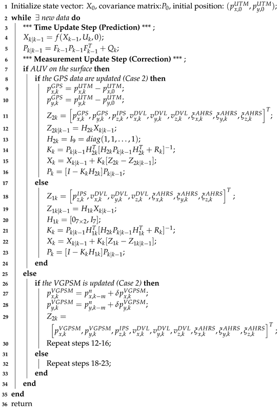
Although the above navigation technologies have suppressed the divergence rate of navigation system errors to a certain extent, they still have certain limitations [40]. For example, deep learning methods rely on a large amount of high-quality data and computing resources. To overcome the above problems, this paper proposes a navigation method that combines the traditional EKF and the virtual GPS model (VGPSM) based on deep sequence learning to provide high-precision and high-update rate navigation information for an autonomous underwater vehicle. The main contributions of this paper are summarized as follows:

• According to the high-quality navigation sensor data, when GPS data are available on the surface, based on the time-series characteristics of the navigation system data, a deep sequence learning model integrating LSTM and Bi-LSTM is constructed to learn the relationship between the GPS data and the DVL and AHRS data in the surface environment, and forms a virtual GPS model, which solves the problem of no GPS signal underwater.
• Observation vectors are constructed for two cases, depending on whether the AUVs have positional aids when performing the mission. The virtual GPS model is updated at the same frequency as the real GPS data. When there is an update in the surface GPS or the underwater VGPSM, the corresponding position is added to the observation vector. Otherwise, the observation vector does not contain position information, which effectively solves the limitations of traditional navigation methods when there is no external position assistance.
• Through experiments on real navigation data, the performance and practical application effects of the proposed method in different situations are verified, which provides new ideas and references for the development of underwater vehicle navigation technology.

The structure of this paper is organized as follows: Section 2 introduces the basic knowledge of navigation system. Section 3 describes the specific implementation process of a virtual GPS model based on deep sequence learning and the proposed methodology. Section 4 conducts experimental design and results, followed by Section 5, which offers an in-depth analysis and discussion of the experimental findings. Finally, Section 6 summarizes the key conclusions and contributions of this study. Through these contents, this study hopes to provide new theoretical and technical support for the development of AUV navigation systems.

2. Navigation System

The AUV navigation system contains functions such as sensor data acquisition and navigation positioning. The data collected using each sensor will be sent to the data center (MOOSDB). The navigation algorithm module, after acquiring the sensor data at the current moment from the MOOSDB, calculates a stable and reliable position, velocity, attitude, and other information in real time, and then sends it to the MOOSDB for the other systems of the AUV to acquire in order to perform the task more accurately. This section focuses on the two coordinate systems and the main onboard sensors of the AUV navigation system in this paper.

2.1. Coordinate System for AUV Navigation

The navigation system in this paper uses both the navigation coordinate system and the body coordinate system, as shown in Figure 1. In general, the position, velocity, attitude, acceleration, and angular velocity of the AUV come from the navigation coordinate system by default, but the velocity and acceleration of the AUV during the control system’s manipulation of the AUV’s movement come from the AUV coordinate system.

Figure 1. The coordinate system and onboard sensors for the AUV navigation system.

The letter n is generally used to denote the navigation coordinate system, whose origin $O^n$ is a point fixed to the Earth, generally starting from a stable position obtained after the navigation system is switched on. The $O^n{X}^n$ axis points geographical north along the tangent direction of the reference ellipsoid meridian, the $O^n{Y}^n$ axis points geographical east along the normal direction of the reference ellipsoid, and the $O^n{Z}^n$ axis forms a right-handed coordinate system with the $O^n{X}^n$ axis and the $O^n{Y}^n$ axis in the local horizontal plane, which is also known as the North-East-Down (NED) coordinate system due to its orientation.

The letter b is generally used to denote the carrier coordinate system, whose origin $O^b$ is fixed at the center of mass and moves with the movement of the AUV. The $O^b{X}^b$ axis is in the same direction as the roll axis of the AUV’s angular motion and points to the front of the AUV. The $O^b{Y}^b$ axis is in the same direction as the pitch axis of the AUV’s angular motion and points to the right of the AUV. The $O^b{Z}^b$ axis is in the same direction as the heading axis of the AUV’s angular motion, and forms a right-handed coordinate system with the $O^b{X}^b$ axis and the $O^b{Y}^b$ axis, also known as the Forward-Right-Down (FRD) coordinate system.

2.2. Onboard Sensors for AUV Navigation

This section focuses on the onboard sensors of the navigation system as shown in Figure 1, as well as their performance parameters and output data types, which are shown in Table 1.

Table 1. Performance parameters and output data types of onboard sensors.

Sensors	Data Type	Parameter	Value
AHRS (Ellipse-A)	$w_x^b$, $w_y^b$, $w_z^b$, $a_x^b$, $a_y^b$, $a_z^b$, ${\xi }_x^b$, ${\xi }_y^b$, ${\xi }_z^b$	Heading	1° RMS
		Pitch	0.2° RMS
		Roll	0.2° RMS
		Update Rate	10 Hz (up to 200 Hz)
DVL (NavQuest 600)	$v_x^b$, $v_y^b$, $v_z^b$, $a{l}_z^b$	Velocity Accuracy	1 m/s
		Altitude Range	0.3–110 m
		Maximum Velocity	20 knot
		Update Rate	1 Hz
GPS (LEA-M8T)	$lat$, $lon$	Position Accuracy	2.5 m CEP
		Acquisition	GPS & BeiDou
		Update Rate	1 Hz
		Cold Starts	25 s
IPS (Valeport)	$p_z^n$	Accuracy	0.01 % Range
		Update Rate	1 Hz

The attitude and heading reference system (AHRS), model Ellipse-A AHRS, provides heading (${\xi }_z^b$), pitch (${\xi }_y^b$), roll (${\xi }_x^b$), three-axis acceleration ($a_x^b$, $a_y^b$, $a_z^b$,), and three-axis angular velocity ($w_x^b$, $w_y^b$, $w_z^b$) for the navigation system. The data of AHRS are mainly obtained based on three-axis gyroscopes, three-axis accelerometers, and three-axis magnetometers. Due to the use of the magnetometer, the AHRS needs to be calibrated for the local magnetic field every time the AUV is tested in a new environment.

The Doppler velocity log (DVL) sensor, model NavQuest 600 micro DVL, is used to provide three-dimensional velocity ($v_x^b$, $v_y^b$, $v_z^b$) and bottom height ($a{l}_z^b$) for the navigation system. The transducer array of DVL adopts a four-beam JANUS configuration, which is able to reduce the adverse effects of AUV motion on DVL measurement, and has a high accuracy in the velocity measurement. The bottom height can assist in determining the validity of DVL data.

The global positioning system (GPS), model LEA-M8T GPS, provides latitude and longitude with no accumulated errors for the navigation system. This sensor can provide high-precision data near the water surface where its antenna is not covered, but it is unable to provide a position underwater due to the rapid decay of radio signals, and this paper focuses on improving this.

The intelligent pressure system (IPS), model miniIPS, provides depth ($p_z^n$) for navigation system. The sensor obtains the current depth with high accuracy based on the effect of water pressure on the resistance value, and can provide it to the AUV continuously.

3. Proposed Method for AUV Navigation

As a commonly used method for AUV navigation, EKF can efficiently handle nonlinear systems with good real-time performance and robustness, but it still inevitably suffers from accumulated errors. Sensor noise and model uncertainty lead to gradual deviations in state estimation over time, resulting in cumulative errors. Therefore, these errors need to be corrected by periodic correction to ensure the long-term accuracy and reliability of the navigation system. The navigation system can use GPS position data for error correction while sailing on the surface, but it cannot be performed underwater. We propose a virtual GPS model based on deep sequence learning to address this issue, which outputs the virtual GPS position during AUV underwater navigation for error correction. This section will describe the proposed method in detail, focusing on the proposed virtual/real GPS-assisted EKF and the virtual GPS model.

3.1. Proposed Navigation Method Based on Virtual/Real GPS

The flowchart of the proposed navigation method based on virtual/real GPS is shown in Figure 2. First, a virtual GPS model is constructed and trained based on sensor data, which is consistent with the update frequency of the GPS data. Then, when the AUV navigates near the water surface, its position is assigned to the measurement vector $Z_{2}k\in {\mathbb{R}}^9$ if there is a GPS data update, corresponding to “Case2” in Figure 2; otherwise, the measurement vector $Z_{1}k\in {\mathbb{R}}^7$ has no two-dimensional (2D) position, corresponding to “Case1”. When the AUV has no GPS data underwater, the VGPSM position is assigned to the measurement vector $Z_{2}k\in {\mathbb{R}}^9$ if there is an update of the virtual GPS model; otherwise, there is no 2D position in the measurement vector $Z_{1}k\in {\mathbb{R}}^7$. Finally, the AUV performs navigation positioning based on the prediction and update steps of the EKF.

Figure 2. The framework of the proposed navigation method for AUVs.

The motion model and measurement model of AUV are shown in Equation (1) and Equation (2), respectively.

$$\begin{array}{c}\hfill X_k=f(X_{k-1},U_k,W_k)\end{array}$$

(1)

$$\begin{array}{c}\hfill Z_k=h(X_k,V_k)\end{array}$$

(2)

$$\begin{array}{c}\hfill W_k\sim N(0,Q_k)\end{array}$$

(3)

$$\begin{array}{c}\hfill V_k\sim N(0,R_k)\end{array}$$

(4)

where $f(·)$ and $h(·)$ represent the motion function and measurement function, respectively, $X_k\in {\mathbb{R}}^9$ is the state vector at time k as shown in Equation (5), $W_k\in {\mathbb{R}}^9$ is Gaussian noise at time k with a mean zero and covariance matrix $Q_k$ as shown in Equation (3), $U_k\in {\mathbb{R}}^6$ is the control vector at time k as shown in Equation (6), $V_k$ is Gaussian noise at time k with a mean zero and covariance matrix $R_k$ as shown in Equation (4), and $Z_k$ is the measurement vector at time k. When there is no update from GPS or VGPSM, $Z_k$ is expressed as $Z_{1k}$ as shown in Equation (7); otherwise, $Z_k$ is expressed as $Z_{2k}$, as shown in Equation (8).

$$\begin{array}{c}\hfill X_k={\left[p_{x,k}^n,p_{y,k}^n,p_{z,k}^n,v_{x,k}^b,v_{y,k}^b,v_{z,k}^b,{\xi }_{x,k},{\xi }_{y,k},{\xi }_{z,k}\right]}^T\end{array}$$

(5)

$$\begin{array}{c}\hfill U_k={\left[a_{x,k}^b,a_{y,k}^b,a_{z,k}^b,w_{x,k},w_{y,k},w_{z,k}\right]}^T\end{array}$$

(6)

$$\begin{array}{c}\hfill Z_{1k}={\left[p_{z,k}^{IPS},v_{x,k}^{DVL},v_{y,k}^{DVL},v_{z,k}^{DVL},{\xi }_{x,k}^{AHRS},{\xi }_{y,k}^{AHRS},{\xi }_{z,k}^{AHRS}\right]}^T\end{array}$$

(7)

$$\begin{array}{c}\hfill Z_{2k}={\left[p_{x,k}^{GPS/VGPSM},p_{y,k}^{GPS/VGPSM},p_{z,k}^{IPS},v_{x,k}^{DVL},v_{y,k}^{DVL},v_{z,k}^{DVL},{\xi }_{x,k}^{AHRS},{\xi }_{y,k}^{AHRS},{\xi }_{z,k}^{AHRS}\right]}^T\end{array}$$

(8)

where

• $p_{x,k}^n$, $p_{y,k}^n$, $p_{z,k}^n$: the position of the x, y, and z axes in the navigation coordinate system.
• $v_{x,k}^b$, $v_{y,k}^b$, $v_{z,k}^b$: the velocity of the x, y, and z axes in the body coordinate system.
• ${\xi }_{x,k}$, ${\xi }_{y,k}$, ${\xi }_{z,k}$: the three-dimensional (3D) attitude of the AUV for roll, pitch, and heading.
• $a_{x,k}^b$, $a_{y,k}^b$$,a_{z,k}^b$: the 3D acceleration of the AUV in the body coordinate system.
• $w_{x,k}$, $w_{y,k}$, $w_{z,k}$: the 3D angular velocities of the AUV.
• $p_{x,k}^{GPS/VGPSM}$, $p_{y,k}^{GPS/VGPSM}$: the position of the x and y axes in the navigation coordinate system from GPS or VGPSM.
• $p_{z,k}^{IPS}$: the position of the z axes in the navigation coordinate system from IPS.
• $v_{x,k}^{DVL}$, $v_{y,k}^{DVL}$, $v_{z,k}^{DVL}$: the 3D velocity in the body coordinate system from DVL.
• ${\xi }_{x,k}^{AHRS}$, ${y,k}^{AHRS}$, ${\xi }_{z,k}^{AHRS}$: the 3D attitude of the AUV for roll, pitch, and heading from AHRS.

The pseudo-code of the proposed method is shown in Algorithm 1. When the navigation system is initialized, the state vector $X_0$ and covariance matrix $P_0$ are set up at the initial moment. At this stage, the current GPS position $(lat,lon)$ is recorded and converted into Universal Transverse Mercator (UTM) coordinates $(p_{x,0}^{UTM},p_{y,0}^{UTM})$. During the AUV navigation process, the system primarily relies on two stages: the time update (prediction) and the measurement update (correction) stages. The correction stage is divided into two scenarios: one where the measurement vector $Z_{1}k\in {\mathbb{R}}^7$ does not include the two-dimensional position, corresponding to Case 1, and another where the measurement vector $Z_{2}k\in {\mathbb{R}}^9$ includes the two-dimensional position, corresponding to Case 2. The detailed procedures for these two scenarios are described in Section 3.1.1 and Section 3.1.2, respectively.

Algorithm 1: The pseudo-code of proposed method

3.1.1. The Prediction Stage of Proposed Navigation Method

The prediction and update of the state vector $X_{k|k-1}$ and the covariance matrix $P_{k|k-1}$ are performed at each time step k according to the update frequency of the navigation system. The prediction steps are consistent with Figure 2, as shown in Equations (9) and (10).

$$\begin{array}{c}\hfill X_{k|k-1}=f(X_{k-1},U_k,0)=\left[\begin{array}{c}{p}_{x,k-1}^n+C_{11}\delta p_{x,k}^b+C_{12}\delta p_{y,k}^b+C_{13}\delta p_{z,k}^b\\ p_{y,k-1}^n+C_{21}\delta p_{x,k}^b+C_{22}\delta p_{y,k}^b+C_{23}\delta p_{z,k}^b\\ p_{z,k-1}^n+C_{31}\delta p_{x,k}^b+C_{32}\delta p_{y,k}^b+C_{33}\delta p_{z,k}^b\\ v_{x,k-1}^b+a_{x,k}^b\delta t\\ v_{y,k-1}^b+a_{y,k}^b\delta t\\ v_{z,k-1}^b+a_{z,k}^b\delta t\\ {\xi }_{x,k-1}+w_{x,k}\delta t\\ {\xi }_{y,k-1}+w_{y,k}\delta t\\ {\xi }_{z,k-1}+w_{z,k}\delta t\end{array}\right]\end{array}$$

(9)

$$\begin{array}{c}\hfill P_{k|k-1}=F_{k-1}{P}_{k-1}{F}_{k-1}^T+Q_k\end{array}$$

(10)

where $\delta p_{x,k}^b$, $\delta p_{y,k}^b$, $\delta p_{z,k}^b$ denote the displacement of the x, y, and z axes in the body coordinate system between time steps $k-1$ and k as shown in Equation (11), $\delta t$ denotes the time between time step $k-1$ and k, $F_{k-1}$ is the Jacobi matrix of the motion function $f(·)$ on the state vector $X_{k-1}$ as shown in Equation (12), and $C_{ij}(1\le i\le 3,1\le j\le 3)$ denotes the data in the i-th row and j-th column of the rotation matrix $C_b^n$ that transform from the body coordinate system to the navigation coordinate system, as shown in Equation (13).

$$\begin{array}{c}\hfill {\Delta P}_k^b=\left[\begin{array}{c}\delta p_{x,k}^b\\ \delta p_{y,k}^b\\ \delta p_{z,k}^b\end{array}\right]=\left[\begin{array}{c}{v}_{x,k-1}^b+{\displaystyle \frac{1}{2}}{a}_{x,k}^b\delta t^2\\ v_{y,k-1}^b+{\displaystyle \frac{1}{2}}{a}_{y,k}^b\delta t^2\\ v_{z,k-1}^b+{\displaystyle \frac{1}{2}}{a}_{z,k}^b\delta t^2\end{array}\right]\end{array}$$

(11)

$$\begin{array}{c}\hfill F_{k-1}={\displaystyle \frac{\partial f(X_{k-1},U_k,0)}{\partial X_{k-1}}}\end{array}$$

(12)

$$\begin{array}{c}\hfill C_b^n=\left[\begin{array}{ccc}cos{\xi }_{y}cos{\xi }_z& -cos{\xi }_{y}sin{\xi }_z& sin{\xi }_y\\ cos{\xi }_{x}sin{\xi }_{y}cos{\xi }_z+cos{\xi }_{x}sin{\xi }_z& -sin{\xi }_{x}sin{\xi }_{y}sin{\xi }_z+cos{\xi }_{x}cos{\xi }_z& -sin{\xi }_{y}cos{\xi }_y\\ -cos{\xi }_{x}sin{\xi }_{y}cos{\xi }_z+sin{\xi }_{x}sin{\xi }_z& cos{\xi }_{x}sin{\xi }_{y}sin{\xi }_z+sin{\xi }_{x}cos{\xi }_z& cos{\xi }_{x}cos{\xi }_y\end{array}\right]\end{array}$$

(13)

3.1.2. The Correction Stage of Proposed Navigation Method

After the prediction stage, the measurement update stage follows. When the AUV is sailing on the surface, if the GPS data are updated at this time, the current GPS position $(la{t}_k^{GPS},lo{n}_k^{GPS})$ is converted to the UTM coordinate position $(p_{x,k}^{UTM},p_{y,k}^{UTM})$; then, the measured position $(p_{x,k}^{GPS},p_{y,k}^{GPS})$, as shown in Equation (14), is obtained and assigned to $Z_{2k}$, and the measured values of IPS, DVL, and AHRS are also assigned to $Z_{2k}$, as shown in Equation (15).

$$\begin{array}{c}\hfill \left[\begin{array}{c}{p}_{x,k}^{GPS}\\ p_{y,k}^{GPS}\end{array}\right]=\left[\begin{array}{c}{p}_{x,k}^{UTM}-p_{x,0}^{UTM}\\ p_{y,k}^{UTM}-p_{y,0}^{UTM}\end{array}\right]\end{array}$$

(14)

$$\begin{array}{c}\hfill Z_{2k}={\left[p_{x,k}^{GPS},p_{y,k}^{GPS},p_{z,k}^{IPS},v_{x,k}^{DVL},v_{y,k}^{DVL},v_{z,k}^{DVL},{\xi }_{x,k}^{AHRS},{\xi }_{y,k}^{AHRS},{\xi }_{z,k}^{AHRS}\right]}^T\end{array}$$

(15)

The measurement value $Z_{2k|k-1}$, as shown in Equation (16), is predicted based on the measurement function $h_2(·)$, where $H_{2k}$ is a nine dimensional identity matrix as shown in Equation (17).

$$\begin{array}{c}\hfill Z_{2k|k-1}=h_2(X_{k|k-1},0)=H_{2k}{X}_{k|k-1}\end{array}$$

(16)

$$\begin{array}{c}\hfill H_{2k}={\displaystyle \frac{\partial h_2(X_{k|k-1},0)}{\partial X_{k|k-1}}}\end{array}$$

(17)

The Kalman gain $K_k$ at time step k can be calculated using Equation (18). Then the state vector $X_k$ and its covariance Matrix $P_k$ are corrected as shown in Equations (19) and (20).

$$\begin{array}{c}\hfill K_k=P_{k|k-1}{H}_{2k}^T{[H_{2k}{P}_{k|k-1}{H}_{2k}^T+R_k]}^{-1}\end{array}$$

(18)

$$\begin{array}{c}\hfill X_k=X_{k|k-1}+K_k[Z_{2k}-Z_{2k|k-1}]\end{array}$$

(19)

$$\begin{array}{c}\hfill P_k=[I-K_k{H}_{2k}]P_{k|k-1}\end{array}$$

(20)

If the virtual GPS model is updated when the AUV is sailing underwater, the measurement position $(p_{x,k}^{VGPSM},p_{y,k}^{VGPSM})$, as shown in Equation (21), is obtained based on the displacement output by VGPSM $(\delta p_{x,k}^{VGPSM},\delta p_{y,k}^{VGPSM})$ and the AUV position $(p_{x,k-m}^n,p_{y,k-m}^n)$ at time step $k-m$, which is assigned to $Z_{2k}$ together with the measurement data of IPS, DVL, and AHRS, as shown in Equation (22).

$$\begin{array}{c}\hfill \left[\begin{array}{c}{p}_{x,k}^{VGPSM}\\ p_{y,k}^{VGPSM}\end{array}\right]=\left[\begin{array}{c}{p}_{x,k-m}^n+\delta p_{x,k}^{VGPSM}\\ p_{y,k-m}^n+\delta p_{y,k}^{VGPSM}\end{array}\right]\end{array}$$

(21)

$$\begin{array}{c}\hfill Z_{2k}={\left[p_{x,k}^{VGPSM},p_{y,k}^{VGPSM},p_{z,k}^{IPS},v_{x,k}^{DVL},v_{y,k}^{DVL},v_{z,k}^{DVL},{\xi }_{x,k}^{AHRS},{\xi }_{y,k}^{AHRS},{\xi }_{z,k}^{AHRS}\right]}^T\end{array}$$

(22)

where m is the number of time steps within one GPS update cycle. Then the updated state vector $X_k$ and its covariance matrix $P_k$ can be obtained based on Equations (18)–(20).

The measurement vector $Z_{1k}$, as shown in Equation (7), does not contain a 2D position if there is no GPS data on the surface and no VGPSM data underwater, which is consistent with the situation of “Case 1” in Figure 2. The measurement value $Z_{1k|k-1}$, as shown in Equation (23), is predicted based on the measurement function $h_1(·)$, where the $7\times 9$ matrix $H_{1k}$, as shown in Equation (24), is the Jacobian matrix of the measurement function $h_1(·)$ with respect to the predicted state vector $X_{k|k-1}$.

$$\begin{array}{c}\hfill Z_{1k|k-1}=h_1(X_{k|k-1},0)=H_{1k}{X}_{k|k-1}\end{array}$$

(23)

$$\begin{array}{c}\hfill H_{1k}={\displaystyle \frac{\partial h_1(X_{k|k-1},0)}{\partial X_{k|k-1}}}\end{array}$$

(24)

The Kalman gain $K_k$ at time step k can be calculated using Equation (25). Then the state vector $X_k$ and its covariance Matrix $P_k$ are corrected, as shown in Equations (26) and (27).

$$\begin{array}{c}\hfill K_k=P_{k|k-1}{H}_{1k}^T{[H_{2k}{P}_{k|k-1}{H}_{1k}^T+R_k]}^{-1}\end{array}$$

(25)

$$\begin{array}{c}\hfill X_k=X_{k|k-1}+K_k[Z_{1k}-Z_{1k|k-1}]\end{array}$$

(26)

$$\begin{array}{c}\hfill P_k=[I-K_k{H}_{1k}]P_{k|k-1}\end{array}$$

(27)

3.2. Virtual GPS Model

Aiming at the problem of an increasing cumulative error in the navigation system without underwater positioning assistance, we propose to use a virtual GPS model, as shown in Figure 3, for the underwater position assistance of the AUV navigation system, in order to slow down the increase in cumulative error.

Figure 3. The flowchart of virtual GPS model based on deep sequence learning.

3.2.1. The Construction of Virtual GPS Model

VGPSM is trained and generated based on deep sequence learning, which comprehensively utilizes long short-term memory and bidirectional long short-term memory to effectively capture long-term dependencies in time-series navigation data, and, when combined with a two-layer neural network to learn the nonlinear relationship between navigation sensor data and GPS data, generates virtual GPS displacement.

The construction process of the virtual GPS model is as follows:

• First, the construction of high-quality datasets. Deep sequence learning models can efficiently handle the effects of nonlinearity and noise, but their training process relies on a large amount of high-quality data. Therefore, based on the data from AHRS, DVL, and GPS, we combine improved incremental smoothing and mapping (iSAM) and an adaptive GPS filter to generate position data that are consistent with the update frequency of the navigation system, and then construct them into a high-quality navigation dataset.
• Then, the structural design of a deep sequence model. Based on the time-series characteristics of navigation data, LSTM, which can capture long-term dependencies, and Bi-LSTM, which considers both forward and backward sequence data, are selected to process navigation sequence data. After that, data integration prediction is carried out by combining a 2-layer fully-connected layer, a Dropout layer, which prevents overfitting, and a Regression layer. Finally, the predicted virtual GPS position can be obtained using the output layer.
• Finally, the training and prediction process of the virtual GPS model. In total, 80% of the navigation dataset constructed above is used for training and 20% is used for testing. The input and output of the dataset are normalized before the training begins. The training process uses the mean square error (MSE) as the loss function, the optimizer is selected as Adam, and the initial learning rate is set to 0.001. After the DVL and AHRS data are processed with the same normalization parameters, they are input into the trained virtual GPSM model to generate the virtual GPS displacement.

Before constructing the navigation dataset, it is necessary to collect and save the data of the same AUV under various trajectories when there is an update of GPS on the surface, including the 3D attitude of DVL, the 2D position of GPS, the 3D acceleration, the 3D angular velocity, and the 3D attitude of AHRS. The update frequency of the navigation system is 10 Hz, and the update frequency of the GPS is 1 Hz. Since the GPS antenna may be covered by waves on the water surface causing drift errors, the above data are put through improved iSAM and the adaptive GPS filter for the navigation computation, and the navigation data with the update frequency of 10 Hz are generated uniformly.

Based on the described procedures, we can construct a dataset ‘NavD’ specifically for AUV navigation. Considering the navigation update frequency, the dataset is sampled at 0.1 s intervals. Taking the j-th row as an example, the input vector $I_j^n$ shown in Equation (28) consists of sensor data including DVL, AHRS, IPS, and GPS with a feature set of 15 in every time step j.

$$\begin{array}{c}\hfill I_j^n=\left[v_{x,j}^{DVL},v_{y,j}^{DVL},v_{z,j}^{DVL},{\xi }_{x,j}^{AHRS},{\xi }_{y,j}^{AHRS},{\xi }_{z,j}^{AHRS},a_{x,j}^{AHRS},a_{y,j}^{AHRS},a_{z,j}^{AHRS},w_{x,j}^{AHRS},w_{y,j}^{AHRS},w_{z,j}^{AHRS},p_{z,j}^{IPS},la{t}_j^{GPS},lo{n}_j^{GPS}\right]\end{array}$$

(28)

The output vector $O_j^n$ of ‘NavD’ shown in Equation (29) includes the northward and eastward positions $(p_{x,j}^n,p_{y,j}^n)$, as well as the northward and eastward displacements $(p_{x,j}^n-p_{x,j-1}^n,p_{y,j}^n-p_{y,j-1}^n)$ at time step j.

$$\begin{array}{c}\hfill O_j^n=\left[p_{x,j}^n,p_{y,j}^n,p_{x,j}^n-p_{x,j-1}^n,p_{y,j}^n-p_{y,j-1}^n\right]\end{array}$$

(29)

Based on the existing dataset ‘NavD’, the relevant portions are selected to construct a specialized dataset “VGD” for the training and testing of the virtual GPS model. As shown in Figure 3, the input sequence $x^{\left(i\right)}$ at time step i is shown in Equation (30).

$$\begin{array}{c}\hfill x^{\left(i\right)}=\left[I_{m\times (i-1)+1}^n(1:12),I_{m\times (i-1)+2}^n(1:12),I_{m\times (i-1)+3}^n(1:12),\dots ,I_{m\times i}^n(1:12)\right]\end{array}$$

(30)

where $I_{i\times m}^n(1:12)$ is the DVL and AHRS data at time step $i\times m$, and m is the number of time steps within one GPS update cycle.

The output vector $y^{\left(i\right)}$ of ‘VGD’ shown in Equation (31) is the northward and eastward displacements of m time steps in the navigation coordinate system, and its output frequency is consistent with GPS.

$$\begin{array}{c}\hfill y^{\left(i\right)}=\left[O_{m\times i}^n(1:2)-O_{m\times (i-1)}^n(1:2)\right]\end{array}$$

(31)

The training of the virtual GPS model is based on the input $x^{\left(i\right)}$ and output $y^{\left(i\right)}$ from the dataset ‘VGD’. The model starts with an input layer, where each sequence contains 10 time steps, with 12 features per time step. The hidden layer is a hybrid gated recurrent neural network (HGRNN) composed of an LSTM and a bidirectional LSTM (Bi-LSTM). The Bi-LSTM layer has 128 units, followed by a unidirectional LSTM layer with 64 units. The output is then passed through a fully connected layer (FC1) with 64 units, followed by a Dropout layer with a dropout rate of 0.5 to prevent overfitting. Afterward, the data go through another fully connected layer (FC2) with 32 units, and finally, the regression layer outputs two features. The model is trained with a batch size of 64, a learning rate of 0.001, and for 100 epochs. The loss function used is Mean Squared Error (MSE), optimized using the Adam optimizer.

The virtual GPS model is imported into the AUV navigation system for the virtual GPS displacement output $y_o^{\left(i\right)}$, as shown in Equation (32), during navigation.

$$\begin{array}{c}\hfill y_o^{\left(i\right)}=\left[\delta p_{x,i}^{VGPSM},\delta p_{y,i}^{VGPSM}\right]\end{array}$$

(32)

where $\delta p_{x,i}^{VGPSM}$ and $\delta p_{y,i}^{VGPSM}$ denote the northward and eastward displacement over m time steps.

3.2.2. Bi-LSTM and LSTM

A hybrid recurrent gated neural network consisting of Bi-LSTM and LSTM is used in the virtual GPS model. The Bi-LSTM, as shown in Figure 4, consisting of forward and backward LSTM, can learn the bidirectional long-term dependencies of sequence navigation data. The structure of the LSTM cell can integrate long-term memory and short-term memory based on gating with different functions.

Figure 4. The structure of Bi-LSTM and LSTM. (a) Bi-LSTM. (b) LSTM.

LSTM is a recurrent neural network (RNN) that can effectively solve the gradient vanishing problem in traditional RNN, and is suitable for time-series-based data prediction. As shown in Figure 4, the LSTM cell consists of an input gate, a forget gate, and an output gate.

As described in the yellow dashed box in Figure 4, the forget gate processes the output $s^{(t-1)}$ of the previous moment and the input $x^{\left(t\right)}$ of the current moment through a sigmoid layer to obtain the activation vector $f^{\left(t\right)}$, shown in Equation (33).

$$\begin{array}{c}\hfill f^{\left(t\right)}=\sigma (W_f{s}^{(t-1)}+U_f{x}^{\left(t\right)}+b_f)\end{array}$$

(33)

As shown in the blue dashed box, the input gate combines $s^{(t-1)}$ and $x^{\left(t\right)}$ through the sigmoid layer to obtain the input gate’s activation vector $i^{\left(t\right)}$, as shown in Equation (34), and through the tanh layer to obtain the cell input activation vector $i_t$, as shown in Equation (35).

$$\begin{array}{c}\hfill i^{\left(t\right)}=\sigma (W_i{s}^{(t-1)}+U_i{x}^{\left(t\right)}+b_i)\end{array}$$

(34)

$$\begin{array}{c}\hfill c_1^{\left(t\right)}=tanh(W_c{s}^{(t-1)}+U_c{x}^{\left(t\right)}+b_c)\end{array}$$

(35)

The light green line represents long-term memory. The forget gate determines the degree to which the long-term memory $c^{(t-1)}$ at $t-1$ moment is forgotten, and the input gate selects the degree to which the short-term memory is increased, which together determine the long-term memory $c^{\left(t\right)}$ of the current moment, as shown in Equation (36).

$$\begin{array}{c}\hfill c^{\left(t\right)}=g_i\ast c_1^{\left(t\right)}+f^{\left(t\right)}\ast c^{(t-1)}\end{array}$$

(36)

As indicated by the pink dashed box, the combination of $s^{(t-1)}$ and $x^{\left(t\right)}$ is passed through the sigmoid layer to obtain the output gate’s activation vector $o^{\left(t\right)}$, as shown in Equation (37). Combined with the tanh layer’s processing of $c^{\left(t\right)}$, the output gate’s activation vector $s^{\left(t\right)}$, as shown in Equation (38), is obtained.

$$\begin{array}{c}\hfill o^{\left(t\right)}=\sigma (W_o{s}^{(t-1)}+U_o{x}^{\left(t\right)}+b_o)\end{array}$$

(37)

$$\begin{array}{c}\hfill s^{\left(t\right)}=o^{\left(t\right)}\ast tanh\left(c^{\left(t\right)}\right)\end{array}$$

(38)

where $W_{\ast }$ and $U_{\ast }$ denote the weight matrices, and $b_{\ast }$ denotes the bias vector parameter.

4. Experimental Results

This section will mainly present the performance of the virtual GPS model and its correction of the navigation system in combination with the real GPS position.

To validate the proposed algorithm, we conducted a series of carefully controlled experiments. The experimental data were collected from the Sailfish AUV, shown in Figure 2, under optimal sea conditions. The datasets used for this validation are ‘NavD’ and ‘VGD,’ as described in Section 3.2.1. The ‘NavD’ dataset, with a time interval of 0.1 s, serves as the foundational dataset from which the ‘VGD’ dataset was derived. ‘VGD’ was constructed by subsampling ‘NavD’ at 1-second intervals to match the GPS update frequency.

The sensor data incorporated in these experiments include 3D attitude, 3D acceleration, and 3D angular velocity from AHRS, 3D velocity from DVL, latitude and longitude from GPS, and depth measurements from IPS. The sensors used in these experiments are detailed in Table 1, which lists their models and key specifications. Furthermore, the primary parameters employed in the experiments are summarized in Table 2.

Table 2. Primary parameters employed in the experiments.

Parameter Name	Symbol	Value	Description
Time Step	$\delta t$	0.1	Time interval for each time step.
Time Interval	m	10	Number of time steps in one GPS update cycle
Initial State Vector	$X_0$	$0_{9\times 1}$	The initial 3D position, velocity, and attitude in navigation coordinate system.
Initial State Covariance	$P_0$	$\left[\begin{array}{c}0.1\ast I_3,0_{3\times 6}\\ 0_{3\times 3},0.01\ast I_3,0_{3\times 3}\\ 0_{3\times 6},0.001\ast I_3\end{array}\right]$	Covariance matrix of initial state error.
Jacobian matrix 1	$H_{1k}$	$\left[0_{7\times 2},I_7\right]$	Jacobian matrix of measurement function $h_1(·)$
Jacobian matrix 2	$H_{2k}$	$I_9$	Jacobian matrix of measurement function $h_2(·)$

4.1. The Results of Virtual GPS Model

The virtual GPS model provides position information for the AUV underwater without GPS assistance to improve the navigation system accuracy. Figure 5 shows the result of the virtual GPS model. The northward and eastward displacement of GPS is taken as the true value, and that of the virtual GPS model is compared in terms of displacement waveform, root mean square error (RMSE), and single-step error.

Figure 5. The result of virtual GPS model (a) Northward Displacement. (b) Eastward Displacement. (c) RMSE of Northward Displacement. (d) RMSE of Northward Displacement. (e,f) Error of Northward and Eastward Displacement.

In Figure 5, the red and blue lines represent the true values of northward and eastward displacement, respectively, and the cyan and magenta lines represent the northward and eastward displacement of the virtual GPS model, respectively. (a) and (b) represent the northward and eastward displacement comparison between the virtual GPS model and the GPS truth. (c) and (d) represent the northward and eastward root mean square error between the virtual GPS model and the ground truth, respectively. (e) and (f) compare the error between the virtual GPS model and the truth in two ways, where (e) shows the error at each step, and (f) shows the statistics of all errors.

In order to analyze the performance of the virtual GPS model specifically, we formed a table, as shown in Table 3, which mainly analyzes the performance of the virtual GPS model in terms of the mean, standard deviation, and median of the errors, as well as the root mean square error.

Table 3. Numerical performance of virtual GPS model.

Type	|Error|-M (m)	|Error|-S (m)	Error-M (m)	Error-S (m)	Error-Med (m)	RMSE (m)
Northward	0.0433	0.032	0.0019	0.0538	0.0021	0.0538
Displacement
Eastward	0.0393	0.0312	−0.0059	0.0498	0.0046	0.0502
Displacement

As shown in Figure 5e, since there are positive and negative errors, we conducted two kinds of analyses on the mean and standard deviation of the errors. One is to take the absolute value of all errors and then solve for the mean (|Error-M|), as shown in Equation (39), and the standard deviation (|Error|-S), as shown in Equation (40). The other is to directly solve for the mean of the errors (Error-M), as shown in Equation (41), and the standard deviation (Error-S), as shown in Equation (42).

$$\begin{array}{c}\hfill {\left|Error\right|}_M={\displaystyle \frac{1}{T}}\sum _{m=1}^T|x_m-{\widehat{x}}_m|\end{array}$$

(39)

$$\begin{array}{c}\hfill {\left|Error\right|}_S=\sqrt{{\displaystyle \frac{1}{T}}\sum _{m=1}^T\left(\right|x_m-{\widehat{x}}_m{|-|Error|}_M{)}^2}\end{array}$$

(40)

$$\begin{array}{c}\hfill Erro{r}_M={\displaystyle \frac{1}{T}}\sum _{m=1}^T(x_m-{\widehat{x}}_m)\end{array}$$

(41)

$$\begin{array}{c}\hfill Erro{r}_S=\sqrt{{\displaystyle \frac{1}{T}}\sum _{m=1}^T{(x_m-{\widehat{x}}_m-Erro{r}_M)}^2}\end{array}$$

(42)

The calculation of RMSE is shown in Equation (43).

$$\begin{array}{c}\hfill RMSE=\sqrt{{\displaystyle \frac{1}{T}}\sum _{m=1}^T{(x_m-{\widehat{x}}_m)}^2}\end{array}$$

(43)

where $x_m$ denotes the true value of northward or eastward displacement at time step m, ${\widehat{x}}_m$ denotes the predicted value of northward or eastward displacement output using the virtual GPS model at time step m, and T denotes the total time steps.

4.2. The Results of Proposed Algorithm

To evaluate the effectiveness of the proposed algorithm, we have meticulously designed three experimental scenarios.

Scenario 1, as depicted in Figure 6, provides continuous GPS assistance throughout the entire operation. In this scenario, both EKF-GPS and the proposed algorithm receive position updates directly from the GPS, while EKF-VGPSM utilizes a virtual velocity model for position correction.

Figure 6. The comparison between proposed method and other algorithms in Scenario 1. (a) AUV trajectory. (b) Position RMSE. (c) Position error. (d) Northward and Eastward error.

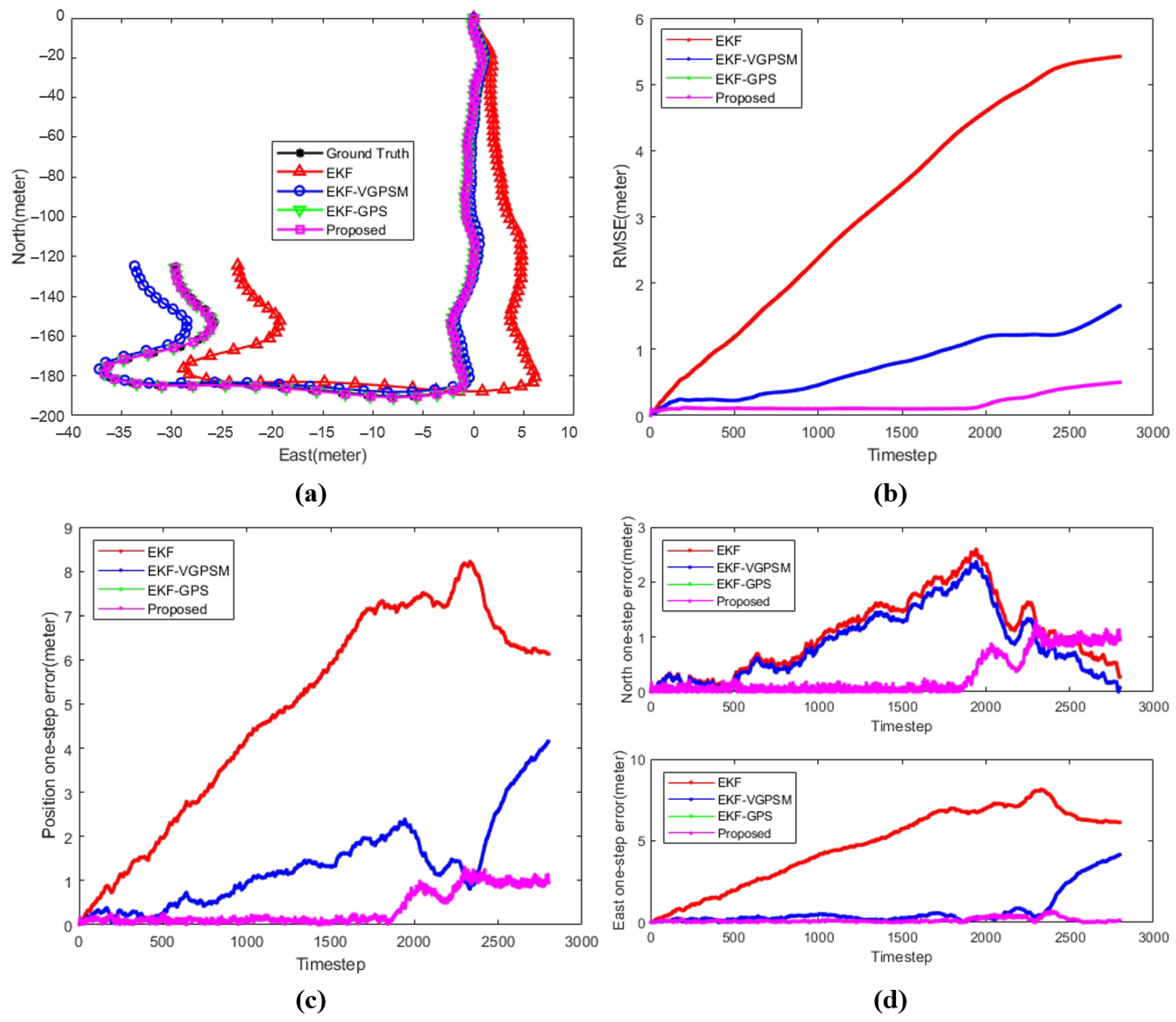
Scenario 2, illustrated in Figure 7, involves GPS assistance only during the first third of the operation, followed by a period without GPS support during the middle third. Specifically, in this scenario, EKF-GPS and the proposed algorithm are aided by GPS during the initial phase. During the subsequent two-thirds of the operation, the proposed algorithm relies on a virtual GPS model for position updates, while EKF-VGPSM depends entirely on the virtual GPS model for the entire duration.

Figure 7. The comparison between proposed method and other algorithms in Scenario 2. (a) AUV trajectory. (b) Position RMSE. (c) Position error. (d) Northward and Eastward error.

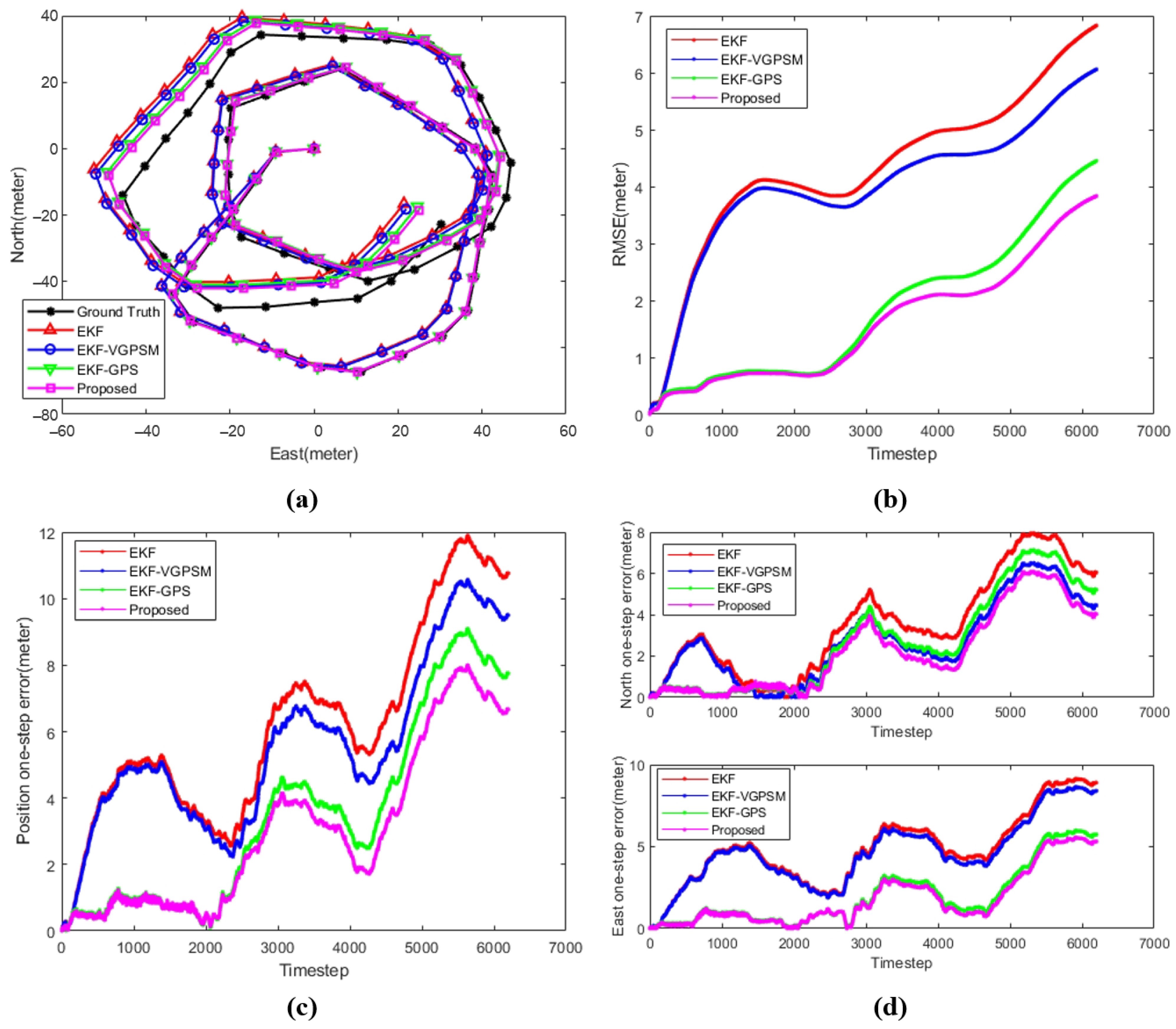
Scenario 3, shown in Figure 8, operates without any GPS assistance for the entire duration. In this case, EKF-GPS behaves identically to a standard EKF without GPS, while the proposed algorithm functions equivalently to EKF-VGPSM, both relying solely on the virtual GPS model for positional updates.

Figure 8. The comparison between proposed method and other algorithms in Scenario 3. (a) AUV trajectory. (b) Position RMSE. (c) Position error. (d) Northward and Eastward error.

These three scenarios are designed to comprehensively assess the performance of the proposed algorithm under varying conditions, particularly focusing on its robustness and accuracy in the absence of real-time GPS data, which is critical for underwater navigation systems.

In Figure 6, Figure 7 and Figure 8, the black line represents the ground truth, the red line denotes the trajectory estimated using the standard extended Kalman filter (EKF), the blue line illustrates the trajectory estimated using the EKF augmented with the virtual GPS model (VGPSM), the green line depicts the trajectory estimated using the EKF with GPS positional assistance (EKF-GPS), and the magenta line represents the trajectory generated using the proposed algorithm. Subfigure (a) shows a trajectory comparison among the aforementioned algorithms against the ground truth. Subfigure (b) compares the root mean square error (RMSE) of the different methods. Subfigure (c) contrasts the single-step error across the algorithms, while Subfigure (d) breaks down the single-step error into the northward and eastward components.

To enhance the clarity of the results presented in Figure 6, Figure 7 and Figure 8, we summarize the key findings in Table 4. This table primarily includes the trajectory length, the root mean square error (RMSE), the endpoint error, the northward error (Error-N), and the eastward error (Error-E) at the endpoint, and the overall navigation accuracy for each scenario. The RMSE represents the root mean square of the displacement errors, calculated as shown in Equation (44). The displacement error at time step i is determined according to Equation (45), and the navigation accuracy is computed using Equation (46). Additionally, the optimal values achieved by each algorithm across the three scenarios are highlighted in bold to facilitate a clearer comparison of the strengths and weaknesses of each method.

$$\begin{array}{c}\hfill RMSE=\sqrt{{\displaystyle \frac{1}{T}}\sum _{i=1}^{T}Erro{r}_i^2}\end{array}$$

(44)

$$\begin{array}{c}\hfill Erro{r}_i=\sqrt{{(x_i-{\widehat{x}}_i)}^2+{(y_i-{\widehat{y}}_i)}^2}\end{array}$$

(45)

$$\begin{array}{c}\hfill Accuracy={\displaystyle \frac{RMSE}{Distance}}\end{array}$$

(46)

where $x_i$ and $y_i$ denote the ground truth of the displacement at time step i in the north and east directions, respectively, ${\widehat{x}}_i$ and ${\widehat{y}}_i$ denote the outputs of the virtual GPS model at time step i in the north and east directions, respectively, T denotes the total number of time steps, and $Distance$ denotes the total distance of this set of data.

Table 4. Numerical performance of different algorithms for AUV navigation.

Data	Distance (m)	Algorithm	RMSE (m)	Error (m)	Error-N (m)	Error-E (m)	Accuracy
Scenario 1	287.33	EKF	5.42	6.14	0.27	6.13	0.01886
		EKF-VGPSM	1.65	4.16	0.07	4.15	0.00574
		EKF-GPS	0.5	0.95	0.94	0.13	0.00174
		Proposed	0.5	0.95	0.94	0.13	0.00174
Scenario 2	641.48	EKF	6.83	10.75	6.04	8.9	0.01065
		EKF-VGPSM	6.06	9.5	4.45	8.39	0.00945
		EKF-GPS	4.45	7.76	5.22	5.74	0.00694
		Proposed	3.8	6.67	4.03	5.31	0.00592
Scenario 3	457	EKF	6.37	7.35	5.06	5.33	0.01394
		EKF-VGPSM	4.51	4.94	3.31	3.67	0.00987
		EKF-GPS	6.37	7.35	5.06	5.33	0.01394
		Proposed	4.51	4.94	3.31	3.67	0.00987

5. Experimental Analysis

5.1. The Performance Analysis of Virtual GPS Model

In order to verify the effectiveness of the virtual GPS model, we first carried out the comparison between the virtual GPS model and the true GPS data in the northward and eastward displacements, the results of which are shown in Figure 5 and Table 3.

From the displacement comparison in (a) and (b), it can be seen that the northward and eastward displacements output by the virtual GPS model are very close to the true displacement values of GPS. From the comparison of the root mean square error in the subfigures (c) and (d), it can be seen that the RMSE of northward and eastward displacements is basically stable at around 0.05 m. Combined with Table 3, the root mean square errors of the virtual GPS model in the north and east directions throughout the entire process are 0.0538 m and 0.0502 m, respectively. From the error comparisons in (e) and (f), it can be seen that the single-step error fluctuates around $-0.1$ m to 0.1 m, and the median error is close to 0 m. Combined with Table 3, it can be seen that the mean and covariance of the errors between the northward displacement and the true value of the virtual GPS model are 0.0019 m and 0.0538 m, respectively, and the mean and covariance of the errors between the virtual GPS model and the true value in northward displacement are 0.0019 m and 0.0538 m, respectively, and those in eastward displacement are −0.0059 m and 0.0498 m, respectively. To show the distribution of the data, the mean of the absolute value of the error is higher than that of the error, and the mean squared error of the absolute value of the error is lower than that of the error.

5.2. The Performance Analysis of Proposed Method

To evaluate the effectiveness of the proposed algorithm, we conducted three experimental scenarios under different conditions. In the first scenario, depicted in Figure 6, both the EKF-GPS and the proposed algorithm operated with continuous GPS assistance throughout the entire process. In this setup, EKF-VGPSM relied on the position data provided by the output of the virtual GPS model. The results clearly show that the navigation accuracy of EKF-VGPSM was significantly better than that of the standard EKF. Moreover, the trajectories produced by both EKF-GPS and the proposed algorithm coincided and were noticeably more accurate than those of EKF-VGPS alone. As summarized in Table 4, the proposed algorithm and EKF-GPS exhibited the smallest root mean square error (RMSE), endpoint error, and eastward error at the endpoint. The proposed algorithm improved navigation accuracy by 90.77 % compared to EKF, primarily due to the continuous GPS support. Additionally, EKF-VGPSM, leveraging the virtual GPS model, achieved a 69.56 % improvement in accuracy over EKF, further validating the effectiveness of the proposed method.

In the second scenario, illustrated in Figure 7, both EKF-GPS and the proposed algorithm were initially assisted by GPS for the first one-third of the experiment. However, during the remaining two-thirds of the time, the EKF-GPS lost its positional assistance, while the proposed algorithm continued to benefit from the virtual GPS model’s output. In the first phase, the errors of both EKF-GPS and the proposed algorithm were minimal due to GPS assistance. However, in the second phase, the error of EKF-GPS began to increase as it lost GPS support. In contrast, the proposed algorithm, aided by the virtual GPS model, maintained significantly lower errors and outperformed all other algorithms. According to Table 4, the proposed algorithm demonstrated the smallest RMSE, endpoint error, and errors in both the northward and eastward directions. The navigation accuracy of the proposed algorithm was improved by 37.77 % compared to EKF, showcasing its robustness even with partial GPS assistance.

In the third scenario, shown in Figure 8, no GPS assistance was available. Under these conditions, EKF-GPS lost its available GPS position data, and its navigation results aligned with those of the standard EKF, as indicated by the overlapping red and green trajectories in the figure. Both EKF-VGPSM and the proposed algorithm relied entirely on the virtual GPS model for positional data, resulting in consistent navigation outcomes, as reflected by the overlapping magenta and blue lines. This scenario effectively compares the navigation performance of EKF and EKF-VGPSM. The results clearly indicate that EKF-VGPSM and the proposed algorithm, both supported by the virtual GPS model, achieved significantly better navigation accuracy than the standard EKF and EKF-GPS. Table 4 confirms that the proposed algorithm reduced the root mean square error to 4.51 m compared to 6.37 m for EKF, resulting in a 29.2% improvement in navigation accuracy.

The effectiveness of the proposed method has been validated through a series of experiments under varying conditions. The results demonstrate that the proposed approach effectively reduces cumulative errors, with navigation accuracy improvements ranging from 29.2% to 69.56% compared to the conventional EKF. Additionally, the virtual GPS model’s output accurately predicts real GPS displacement changes, with root mean square errors of 0.0538 m northward and 0.0502 m eastward, respectively. These experimental results robustly demonstrate the proposed method’s effectiveness in improving navigation accuracy.

5.3. Error Analysis

The primary sources of error stem from sensor inaccuracies and model limitations. AHRS, while essential for orientation data, can introduce drift over time due to inherent biases and noise in gyroscope and accelerometer readings. DVL, used to measure velocity, can suffer from inaccuracies in low-quality bottom lock or turbulent conditions, leading to velocity estimation errors. GPS, although accurate, can introduce errors due to multipath effects or signal loss, especially in challenging underwater environments.

In the virtual GPS model, errors may arise from the integration of these noisy sensor data, where slight inaccuracies in velocity or orientation measurements can accumulate over time, leading to larger discrepancies. The proposed algorithm mitigates some of these errors through its innovative use of deep neural networks, which likely improves the sensor fusion process. However, the residual errors observed, such as the fluctuations in single-step errors and the slight biases in displacement predictions, indicate that the model could still be susceptible to overfitting or insufficient generalization in diverse conditions.

Overall, while the virtual GPS model and the proposed method significantly enhance navigation accuracy, particularly when GPS data are sparse or unavailable, the errors observed underscore the need for continued refinement in sensor fusion algorithms and model robustness to achieve even higher precision in underwater navigation.

5.4. Computational Complexity Analysis

The computational complexity of the extended Kalman filter primarily hinges on the matrix operations performed during the prediction and correction steps. Let n denote the dimension of the state vector, and o the dimension of the observation vector. The prediction step involves matrix multiplication and addition, leading to a complexity of $O\left(n^2\right)$. The correction step requires matrix inversion and multiplication, with a complexity of $O\left(n^3\right)$. Therefore, the overall complexity for one EKF iteration is $O\left(n^3\right)$.

The virtual GPS model, which integrates Bi-LSTM and LSTM networks, has its computational complexity determined by the number of LSTM units, the sequence length, and the structure of the fully connected layers. Let d represent the input feature dimension, T the sequence length, u the number of LSTM units, and p and q the number of units in the fully connected layers. Given the bidirectional nature of Bi-LSTM, the complexity for this layer is $O\left(2md{u}^2\right)$. For the LSTM layer, processing the sequence unidirectionally yields a complexity of $O\left(md{u}^2\right)$. The fully connected layer computes the output from the LSTM units to the final regression layer, with a complexity of $O(up+pq+2q)$. Thus, the total complexity for processing a sequence through VGPSM is $O\left(md{u}^2\right)$, assuming the fully connected layers and dropout do not significantly affect the complexity.

In practical AUV navigation applications, real-time performance is of paramount importance. The computational complexity of the EKF under standard conditions is $O\left(n^3\right)$. When invoking the VGPSM every m time step, the complexity increases by $O\left(md{u}^2\right)$. While the introduction of VGPSM enhances navigational accuracy, it simultaneously imposes additional demands on computational resources. However, with the support of modern hardware, this level of computational complexity remains within an acceptable range. Specifically, by employing extended time steps m and leveraging efficient parallel computing frameworks, the method can meet the demands of most real-time AUV navigation tasks. Consequently, this approach successfully maintains high accuracy while still offering a significant real-time advantage.

6. Conclusions

To address the issue of increasing navigation errors in low-cost AUV without assisted positioning underwater, this paper introduces a virtual GPS model (VGPSM) based on deep sequence learning. By integrating VGPSM with the extended Kalman filter (EKF), the proposed approach provides a high-precision navigation solution for AUVs. The model leverages time-series data from sensors such as AHRS and DVL during surface navigation. It learns the relationship between these sensor inputs and GPS data using a hybrid architecture of LSTM and Bi-LSTM networks, which are particularly suited for processing and predicting time-series data. The VGPSM generates virtual GPS displacements updated at the same frequency as real GPS data. During underwater navigation, these virtual GPS displacements are utilized as measurements to assist the EKF in state estimation, significantly improving the accuracy and robustness of the navigation system.

However, this study presents certain limitations that warrant consideration. Firstly, the navigation datasets used for training and validation were obtained from a single AUV operating under favorable sea conditions. As a result, the generalizability of the model across different AUV platforms and in more challenging or variable marine environments remains uncertain. Additionally, the model’s computational efficiency requires further optimization to ensure its viability for deployment in real-world scenarios, where computational resources may be limited, and real-time processing demands are more stringent.

Future work will focus on addressing these limitations to enhance the robustness and applicability of the proposed method. Specifically, we aim to diversify the training datasets by incorporating data from multiple AUVs operating under varied environmental conditions, thereby improving the model’s adaptability and performance across diverse scenarios. Furthermore, we will explore advanced optimization techniques to reduce computational overhead, enabling the system to operate more efficiently across a broader range of hardware platforms.