Intelligent Queue Scheduling Method for SPMA-Based UAV Networks

Abstract

Static Priority-based Multiple Access (SPMA) is an emerging and promising wireless MAC protocol which is widely used in Unmanned Aerial Vehicle (UAV) networks. UAV (Unmanned Aerial Vehicle) networks, also known as drone networks, refer to a system of interconnected UAVs that communicate and collaborate to perform tasks autonomously or semi-autonomously. These networks leverage wireless communication technologies to share data, coordinate movements, and optimize mission execution. In SPMA, traffic arriving at the UAV network node can be divided into multiple priorities according to the information timeliness, and the packets of each priority are stored in the corresponding queues with different thresholds to transmit packet, thus guaranteeing the high success rate and low latency for the highest-priority traffic. Unfortunately, the multi-priority queue scheduling of SPMA deprives the packet transmitting opportunity of low-priority traffic, which results in unfair conditions among different-priority traffic. To address this problem, in this paper we propose the method of Adaptive Credit-Based Shaper with Reinforcement Learning (abbreviated as ACBS-RL) to balance the performance of all-priority traffic. In ACBS-RL, the Credit-Based Shaper (CBS) is introduced to SPMA to provide relatively fair packet transmission opportunity among multiple traffic queues by limiting the transmission rate. Due to the dynamic situations of the wireless environment, the Q-learning-based reinforcement learning method is leveraged to adaptively adjust the parameters of CBS (i.e., idleslope and sendslope) to achieve better performance among all priority queues. The extensive simulation results show that compared with traditional SPMA protocol, the proposed ACBS-RL can increase UAV network throughput while guaranteeing Quality of Service (QoS) requirements of all priority traffic.

1. Introduction

Unmanned Aerial Vehicle (UAV) networks, as a type of distributed and self-organizing wireless system, interconnect mobile aerial nodes through advanced networking architectures, such as hierarchical ad hoc structures and clustered topologies [1,2]. UAV networks, also known as drone networks, refer to a system of interconnected UAVs that communicate and collaborate to perform tasks autonomously or semi-autonomously. These networks leverage wireless communication technologies to share data, coordinate movements, and optimize mission execution. These networks synergize real-time situational awareness, rapid deployment, and coordinated operations to achieve mission-critical performance. This technological evolution positions UAV networks as critical infrastructure for smart cities, planetary-scale IoT, and next-generation battle networks.

As a pivotal technology in UAV networks, the Medium Access Control (MAC) protocol plays a critical role in efficiently allocating limited channel resources between network nodes [3,4]. In UAV networks, where nodes share an equal transmission channel, MAC protocols must ensure Quality of Service (QoS), fairness, and compliance with latency and reliability requirements for various services. However, conventional MAC protocols such as Time Division Multiple Access (TDMA) [5] and Carrier Sense Multiple Access with Collision Avoidance (CSMA/CA) [6] face inherent challenges in dynamic UAV environments. TDMA relies on rigid time slot allocations with guard intervals to avoid interference, which introduces synchronization overload and inefficient resource utilization, particularly in scenarios with rapidly changing network topologies or fluctuating traffic loads. CSMA/CA, while collision-averse through carrier sensing and backoff mechanisms, suffers from hidden terminal issues, unbounded latency under high contention, and scalability limitations in dense UAV deployments. These shortcomings degrade network adaptability, spectral efficiency, and real-time performance, hindering their applicability to mission-critical UAV operations. To address these limitations, Statistic Priority-based Multiple Access (SPMA) has emerged as a promising alternative, leveraging dynamic priority scheduling and statistical multiplexing to enhance channel utilization while guaranteeing deterministic latency and reliability for heterogeneous services in UAV networks [7,8]. Compared to the traditional MAC protocols, SPMA, which has the capability of multi-priority QoS, can achieve relatively lower transmission delay and guarantee a 99% one hop first-time success rate with the highest priority traffic [9].

In the context of SPMA, the Channel Occupancy Statistic (COS) metric is utilized to regulate the access modes, enabling the concurrent existence of multiple packets on a shared channel. The main section of the SPMA protocol in UAV networks is shown in Figure 1. In UAV networks, as the number of nodes (drones) increases, network traffic and data prioritization become critical to maintaining efficiency, reliability, and Quality of Service (QoS). Since UAV networks handle diverse data types (e.g., real-time video, telemetry, emergency alerts), priority-based scheduling ensures that critical data is transmitted first. In UAV networks, the high priority traffic includes emergency signals and control commands, which are used for collision avoidance. The medium priority traffic includes real-time video and sensor data, which are used for surveillance. The low priority traffic includes non-critical telemetry and logs, which are used for routine status updates. The performance of multi-priority traffic in UAV networks is impacted by scalability problem, such as increased network congestion, higher routing overhead, and uneven traffic distribution. In the SPMA protocol, service types are set, packetization rules are formulated, services are divided, and priorities are assigned. Subsequently, the service-type information is added to the packet header field for parsing, thereby marking the priority of data packets. As in Figure 1, each UAV node receives the data packets (these packets are generated in the UAV node or transmitted from the neighbourhood UAV node), and allocates them into the corresponding traffic queues. The SPMA protocol sets different traffic queues with designated thresholds. When a highest-layer packet like Priority 0 packet enters the data link layer, it is queued in the corresponding priority queue. Then, if the COS falls below the threshold, the packet can be immediately transmitted. In contrast, the node enters the random backoff state, during which it reevaluates the COS upon completion. Throughout this backoff period, any lower priority packets like Priority 1 and Priority 2 packets that are queued are held until the Priority 0 packets are either transmitted or reach their expiration. If the COS is lower than the threshold, the backoff is canceled. Through strategic control of transmission intervals for each packet, the SPMA protocol adapts to channel load, consequently improving overall success rates. However, during instances of significant network congestion, higher-priority packets will take precedence in transmitting over lower-priority packets. A large number of lower-priority packets wait for a timeout and then are discarded.

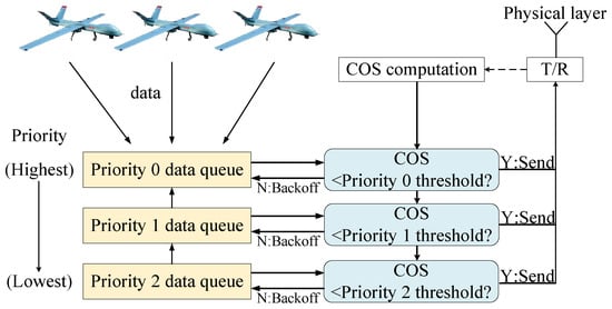
Figure 1. Illustration of SPMA protocol of UAV networks.

As far as we know, there has been some research on SPMA, mainly on mechanism design and performance analysis. These works make efforts to enhance the efficiency of SPMA and offer valuable insights for system design by leveraging assessments of network performance. In [10], a novel improved algorithm called traffic statistic (TSMP-MAC) is proposed, which does not need take the COS metric into account. In [11], a analytical model combining temporal and spatial dimension is designed to obtain better performance. However, all of the above studies ignore the opportunity of lower-priority packet transmission. In UAV networks, lower-priority services are equally crucial and need to satisfy the QoS requirements. The existing fully preemptive mechanism in SPMA only pays attention to the higher-priority packet transmission, but entirely ignores lower-priority services. The transmission delay of lower-priority data packets greatly increases beyond the limit, and the packets may even be dropped. As a result, the hunger phenomenon of lower-priority packets is intensified. Thus, the previous SPMA schemes are not flexible to guarantee QoS requirements for all priority traffic, and it is hard to configure the parameters of SPMA to achieve this objective. In addition, current queue scheduling strategies, while effective in traditional wired or static wireless networks, exhibit critical shortcomings when applied to SPMA-based UAV networks. The static threshold-based prioritization lacks adaptability to dynamic channel conditions and the centralized scheduling paradigms are impractical in distributed UAV networks.

To address this issue, in this paper we propose an intelligent queue scheduling method of Adaptive Credit-Based Shaper with Reinforcement Learning (ACBS-RL) to tackle the unfair transmission of all priority packets in SPMA. The objective of ACBS-RL is to enhance the performance of lower-priority traffic and alleviate the hunger phenomenon of lower-priority packets. In ACBS-RL, the Credit-Based Shaper (CBS) is leveraged instead of a strict priority mechanism in SPMA to guarantee the opportunity of lower-priority packet transmission among multiple traffic queues. CBS is a traffic control mechanism that manages data traffic by allocating credit values. It employs the value of credit adjusted by $idleslope$ and $sendslope$ rate to control the transmission of packets in queues. Due to the dynamic situations of wireless environment, the Q-learning method is utilized to adaptively adjust the parameters of CBS to improve the QoS of low priority queues while ensuring throughput.

The main technique contributions of our work can be summarized as follows:

• We propose a method named ACBS-RL to address the unfair transmission problem of SPMA in UAV networks. We leverage CBS to determine the transmission sequence of queues by the value of credit instead of priority.
• We employ the Q-learning method to dynamically adjust the parameter of the CBS in ACBS-RL to achieve better performance.
• We conduct extensive simulations to evaluate the performance of proposed ACBS-RL. The simulation results confirm the performance of ACBS-RL.

The rest of this paper is organized as follows. In Section 2, we briefly review the literature related to our work. In Section 3, we give the motivation and formulate our problem. The details of ACBS-RL are shown in Section 4. In Section 5, extensive experiment results are given to show the good performance of ACBS-RL. Lastly, we conclude and summarize the paper in Section 6.

2. Related Work

Recently there has been plenty of research on SPMA; most of these studies can be categorized as mechanism design and performance analysis. The goal of the former is to improve the efficiency of SPMA, while the latter is centered around offering design recommendations by evaluating crucial system metrics related to network performance. Additionally, recent research has predominantly focused on queue scheduling strategies involving cross-layer integration and intelligent decision-making. There are also many works about traditional MAC protocols for UAV networks. In this section, we provide an extensive review of the existing research, mainly from the following four aspects.

Mechanism Design of SPMA: In the field of mechanism design, the key parameters of SPMA like COS, backoff schemes, and Statistical Sliding Window (SSW) length are usually considered for optimization [12,13]. In [12], Gao et al. designed a queuing model to analyze protocol performance and proposed a parameter optimization method based on reinforcement learning. A nonpreemptive M/M/1/K queuing model is proposed. And the formulas to analyze the loss rate and delay of different priority traffic in SPMA are derived. By setting percentile scoring criteria to evaluate the performance of SPMA protocol, the system state, action, reward function, and Q-value function in the Q-learning algorithm are designed and implemented. The methods above have many hyperparameters, so it is difficult to design an algorithm under various traffic volumes. In [13], Liu et al. presented a random backoff algorithm. Compared with the Binary Exponential Backoff (BER) algorithm, the backoff time needs to be recomputed at each time and cannot rise due to packet collision, which is suitable for the scenarios of SPMA multi-channel state; furthermore, the channel occupancy factor is not considered. However, these works do not consider the parameters directly related to lower-priority queues, which in turn are related to the hunger phenomenon.

Performance Analysis of SPMA: There have been many studies focusing on performance analysis in SPMA protocol, in which both the temporal arrival of different priorities services and the spatial randomness of node locations are important. The available analytical frameworks were suggested with an emphasis on either the temporal aspect [12] or the spatial aspect [14]. In [8], Liu et al. proposed a straightforward but precise analytical model for calculating the Slot Transmission Probability (STP) under the assumption of saturated input. By utilizing the STP, the key system properties such as mean delay, packet loss rate, throughput, and other relevant metrics are derived. In [14], Zhang et al. quantified the superiority of directional antennas in SPMA networks. In [15], Zhang et al. proposed an analytical framework for examining the performance of SPMA from a spatial standpoint with tools derived from stochastic geometry. The closed-form expressions of some key performance metrics, including MAP and packet success probabilities of different priority services, are derived in a randomly deployed SPMA network by the framework. However, all of the above studies only evaluate the performance of SPMA but never take the QoS of lower-priority queues into consideration.

Queue Scheduling Strategies: The queue scheduling strategies play a pivotal role in managing resource allocation and ensuring QoS across heterogeneous networks. In [16], He et al. proposed a cross-layer optimization framework that jointly addresses user scheduling and beamforming design in multi-cell joint transmission networks, ensuring strict QoS guarantees. In [17], Wang et al. introduced a deep reinforcement learning (DRL) framework for autonomous dynamic multi-channel access in wireless networks, enabling devices to learn optimal channel selection strategies without prior knowledge of traffic patterns or explicit coordination. By training an end-to-end DRL agent to maximize long-term network utility under dynamic interference and contention, the proposed approach significantly improves throughput and reduces latency compared to rule-based and static channel allocation methods in multi-user scenarios.

MAC Protocol for UAV Networks: Since the topology of UAV networks is highly dynamic, the traditional MAC protocol needs to demonstrate flexibility and adaptability to the mobility of UAV nodes. In [18], Chen et al. proposed a novel propagation delay-aware access scheme named LDMAC. The proposed algorithm is suitable for long-distance UAV networks. The LDMAC is a joint optimization of random access and collision-free time slot allocation. In [19], Feng et al. proposed a multi-channel cognitive MAC protocol, named CogMOR-MAC. The proposed algorithm is based on Multi-channel Opportunistic Reservation (MOR) mechanism. The MOR mechanism is focused on dealing with the rendezvous problem and improving resource efficiency with only one radio. In [20], Li et al. proposed a new analysis model to solve the communication heterogeneous problem in UAV networks. A modified three-dimensional Markov chain model adopting the quitting probability and cluster division is presented for the performance analysis. In addition, an improved CSMA/CA protocol is proposed which fully considers the various access time of UAV nodes and adjusts the timeslot resources among UAV nodes in different clusters. However, these traditional MAC protocols, while addressing specific challenges in UAV networks, lack explicit mechanisms for fine-grained priority differentiation of diverse traffic types, and their adaptability to rapid changes in node mobility and traffic load in highly dynamic UAV network topologies remains limited.

Different from the previous works, our work in this paper is aimed at solving the unfair effects caused by the priority transmission evaluation mechanism in SPMA protocol. We attempt to dynamically adjust the parameter of our algorithm by implementing CBS. Additionally, the CBS parameter is dynamically adjusted by Q-learning method. As far as we know, this is the first study to achieve a good tradeoff among all priority packets in SPMA. Therefore, the network throughput of SPMA can be improved while guaranteeing QoS requirements of all priority traffic.

3. Motivation and Problem Formulation

In this section, we describe the motivation for our work based on some examples in Section 3.1, and then formulate the problem to be solved in Section 3.2. For clear presentation, all the notations used in this paper are summarized in Table 1.

Table 1. Notations used in this paper.

Notation	Description
N	The number of UAV nodes
$islp$	The increase rate of credit value for a queue when it is idle
$sslp$	The decrease rate of credit value for a queue when it sends packets
$isl{p}^{\prime }$	The value of $islp$ updated by action a
$ssl{p}^{\prime }$	The value of $sslp$ updated by action a
${\tau }_i$	The head waiting delay requirement for Queue i
$t_i$	The actual head waiting delay for Queue i
L	The packet size for simulation
$T_{sim}$	The simulation duration
$COS$	Channel Occupancy Statistics
$Th$	The threshold at which each priority queue can send packets
$S_i$	The throughput of node i
C	The set of credit value for all priority queues
$C^{\prime }$	The set of credit value for all priority queues in the descending order
T	The transmission time of a packet
$c_{max}$	The maximum credit of value
$Mq$	The ID of queue which has the maximum credit value $c_{max}$
$Tq$	The ID of queue which is ready to transmit
$Q(s,a)$	The Q-value table of Q-Learning algorithm
a	The action adjusting the value of $islp$, $sslp$
Q	The list of all priority queues
$r_t$	The reward for parameter adjusting of time t
$\alpha$	The learning rate
$\gamma$	The discounted factor
R	The total rewards in Q-learning
$Dela{y}_i$	The queuing delay of Queue i
$Los{s}_i$	The packet loss rate of Queue i
$su{m}_i$	The total number of priority i packets transmitted
$t_{leave}$	The time when the packet is dequeued
$t_{arrive}$	The time when the packet is enqueued
$losssnu{m}_i$	The number of lost packet for priority i
$sendnu{m}_i$	The number of successfully transmitted packets for priority i
$scor{e}_{delay}$	The score for the queuing delay of packets
$scor{e}_{loss}$	The score for the packet loss rate
$T_{max}$	The maximum waiting time of packets
$\delta$	The parameter adjusting importance factor for delay
$\beta$	The parameter adjusting importance factor for packet loss
$w_i$	The weight of $scor{e}_i$

3.1. Motivation Example

We give an example in Figure 2 to illustrate our motivation. In the task queue of Figure 2a, there is a node in SPMA with three queues prioritized as 0–2 from top to bottom. Suppose that currently there are a total of 12 data packets in the queues, with 4 packets in Queue 0, 4 packets in Queue 1, and 4 packets in Queue 2. Each packet is given a packet ID. The size of each packet is the same and the transmission time for a packet after dequeuing is 1 ms. In this example, we pay attention to the transmission scenario of lower-priority packets when higher-priority packets come into the queue. Meantime, to assess the QoS of each queue in the network, queuing delay is introduced as a metric for quantifying QoS. The queuing delay is the total waiting time for packets to be dequeued for transmission after being queued. It is required that the queuing delay for packets in Queue 0 be 5 ms, Queue 1 be 6 ms, and Queue 2 be 8 ms.

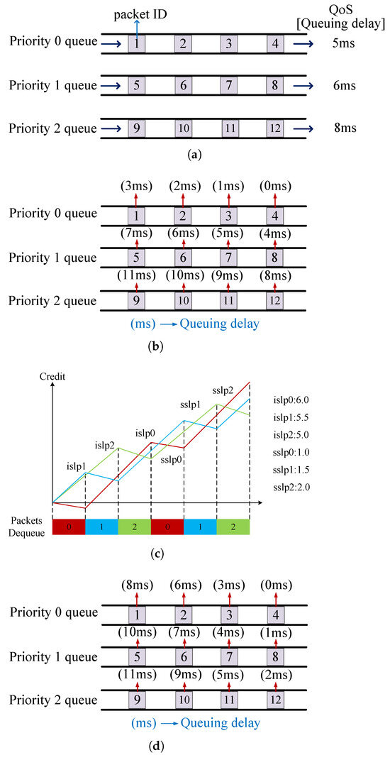
Figure 2. Motivation examples. (a) Task queue. (b) The traditional SPMA algorithm. (c) The CBS mechanism. (d) The ACBS-RL algorithm.

Figure 2b shows the traditional SPMA algorithm in Figure 2a. The order of dequeuing for every packet is 4 → 3 → 2 → 1 → 8 → 7 → 6 → 5 → 12 → 11 → 10 → 9. In the traditional SPMA algorithm, the highest priority packets are transmitted firstly and the average queuing delay of highest priority queue is 1.5 ms. Clearly, the highest priority packets meet the corresponding queuing delay requirement. Other priority packets wait until all highest priority packets are transmitted completely. Then, packets from Queue 1 start to transmit and the average queuing delay of Queue 1 is 5.5 ms. After Queue 1 is empty, packets from Queue 2 are transmitted last and the average queuing delay of Queue 2 is 9.5 ms. The packets from Queue 1 meet the QoS requirement but the packets from Queue 2 wait too long in the queue. Upon analysis, it is observed that packets of Queue 2 fail to meet the queuing delay requirement.

The model of CBS is shown in Figure 2c. In CBS, which is part of the IEEE 802.1Qav standard for Time-Sensitive Networking (TSN), the terms $idleslope$ and $sendslope$ are critical parameters that control the transmission behavior of traffic queues. $idleslope$ (also called increasing slope) represents the rate at which credit increases when the queue is not transmitting (idle), which determines how quickly the CBS replenishes credit for a given traffic queue when no packets are being sent. $sendslope$ (also called decreasing slope) represents the rate at which credit decreases when the queue is transmitting. CBS sets the value of credit to control the sending rate of each priority queue. The value of credit is updated according to the transmission of the packets. Specifically, each priority queue is given the values of credit, $idleslope$ and $sendslope$. The values of credit are utilized to determine which priority packets to be sent. The $idleslope$ and $sendslope$ are used to adjust the values of credit. When a packet is ready to be sent, the credit of the corresponding queue decreases with the rate of $sendslope$. At the same time, the credit of other queues increases with the rate of their own $idleslope$. After the packet is transmitted completely, the credits of all queues are compared to select the maximum. The maximum is used to determine the next queue to transmit a packet. Consequently, the CBS mechanism efficiently arranges task scheduling and resource allocation.

Figure 2d shows the ACBS-RL algorithm. The order of dequeuing for every packet is 4 → 8 → 12 → 3 → 7 → 11 → 2 → 6 → 1 → 10 → 5 → 9. In the ACBS-RL algorithm, the initial values of credit for all queues are set to 0. As shown in Figure 2c, Queue 0 has an $islp$ of 6 and an $sslp$ of 1. Queue 1 has an $islp$ of 5.5 and an $sslp$ of 1.5. Queue 2 has an $islp$ of 5 and an $sslp$ of 2. The following is the specific step-by-step illustration:

• When transmission begins, due to the same credit of each queue, the packet from the highest priority Queue 0 is the first to be transmitted.
• During this period, the credit of Queue 0 decreased to −1 based on $sslp0$, while the credit of Queues 1 and 2, respectively, increased to 5.5 and 5 based on $islp1$ and $islp2$.
• After the transmission is finished, the credit of Queue 1 is at its maximum and the Priority 1 packet start to dequeue.
• During this time, the credit of Queue 1 decreases to 4, while the credits of Queue 0 and 2 become 5 and 10, respectively.
• Then Queue 2 becomes the next transmission queue and all queues follow this mechanism until all packets are sent.

The average queuing delay of Queue 0 is 4.25 ms, which is longer than SPMA. However, the packets from Queue 0 meet the QoS requirement. The average queuing delay of Queue 1 is 5.5 ms, the same as SPMA, and the average queuing delay of Queue 2 is 6.75 ms, which improves the transmission quality and guarantees the QoS requirement.

3.2. Problem Formulation

In a SPMA-based UAV network, each UAV node utilizes the priority packet queue mechanism to store and transmit data packets. In this study, our objective is to maximize throughput of the whole UAV network while guaranteeing the QoS requirement of all traffic queues.

We define the queuing delay model as follows. The actual queuing delay $t_i$ for queue i is defined as the average time a packet waits in the queue:

$$t_i={\displaystyle \frac{{\sum }_{r=1}^{su{m}_i}(t_{leave}-t_{arrive})}{su{m}_i}}$$

(1)

We define the queuing delay requirement ${\tau }_i$ and the QoS requirement constraint that should be satisfied:

$$t_i\le {\tau }_i$$

(2)

Meanwhile, we define the throughput model as follows. The throughput of node i is determined by the number of successfully transmitted packets, and the total network throughput is the sum of the throughputs across all nodes:

$$S_i={\displaystyle \frac{sendnu{m}_i\times L}{T_{sim}}}$$

(3)

In addition, we define the packet loss model as follows. To ensure that QoS is comprehensive, we also consider packet loss rate:

$$Los{s}_i={\displaystyle \frac{losssu{m}_i}{sendsu{m}_i+losssu{m}_i}}$$

(4)

The problem is reformulated as a Markov Decision Process (MDP) to enable RL-based optimization, aiming to maximize long-term cumulative rewards while satisfying QoS constraints. We model the state space (S) and the state is defined by the current $islp$ and $sslp$ of all priority queues:

$$s=(isl{p}_1,ssl{p}_1,isl{p}_2,ssl{p}_2,\dots \dots ,isl{p}_n,ssl{p}_n)$$

(5)

We model the action space (A) and the actions involve adjusting $islp$ and $sslp$ to balance credit values across queues:

$$a=({\theta }_{i1},{\theta }_{s1},{\theta }_{i2},{\theta }_{s2},\dots ,{\theta }_{in},{\theta }_{sn})$$

(6)

Finally, we model the reward function ($r_t$), and the reward integrates scores for queuing delay and packet loss to reflect QoS and throughput performance:

$$r_t=\sum _{i=1}^n{w}_i(\delta scor{e}_{delay,i}+\beta scor{e}_{loss,i})$$

(7)

Our goal is to learn an optimal policy $\pi$ that maximizes the discounted cumulative reward:

$$\begin{array}{cc}\hfill & ma{x}_{\pi }{\mathbb{E}}_{\pi }[\sum _{t=0}^{\infty }{\gamma }^t{r}_t]\hfill \\ \hfill & subjectto:\left(2\right)\hfill \end{array}$$

(8)

4. Algorithm Design

In this section, we present an ACBS-RL algorithm based on the CBS mechanism to alleviate the hunger phenomenon in packet transmission for SPMA.

Algorithm 1 shows how packets from different priority queues are sent in ACBS-RL. The inputs are the value of credit C for each queue, the transmission time of packet T, the $idleslpoe$, and the $sendslope$. In line 1, the initialization for algorithm is performed in $Procedure$$Initialization$ (see in Algorithm 2). Then the action a for current state is chosen by $ϵ-greedy$ strategy (line 4). The $ϵ-greedy$ shows that there is a small positive number $ϵ$ as the probability to randomly select an action. And the action with the largest movement has the left probability $1-ϵ$. In line 5–6, the current $islp$, $sslp$ are updated by a. Specifically, the node chooses the largest reward action with probability $ϵ$, but randomly selects an action from the action pool with probability $1-ϵ$. The credit sets C of all queues are sorted in the descending order to get $C^{\prime }$ and the ID of queues with the highest credit is stored in maximum credit queues $Mq$ (line 7–9). If there are multiple queues stored in $Mq$, the queue with the highest priority would be selected as the transmission queue $Tq$ (line 10–14). In line 15–22, the packet is pulled from the queue $Tq$ and sent if its corresponding $COS$ is smaller than $Th$. Otherwise, it waits until $COS$ decreases. In line 23, the C are updated by $CBS$$function$ (see in Algorithm 3) while the packet is transmitted. In line 24, after transmission, the $Q(s,a)$ are updated by $Q-learningfunction$ (see in Algorithm 4). After that, the training time $N_{train}$ of $Q-learning$ is compared with the maximum training time $N_{max}$. If $N_{train}$ does not reach the required training time, the next packet is transmitted with the new parameter (line 25–27). Finally, all queues are empty and the ACBS-RL algorithm ends (line 28).

Algorithm 1 ACBS-RL algorithm.

1: Input: T, $Th$, $islp$, $sslp$.   2: Output: All the packets of in priority queues are sent.   3: Execute Procedure Initialization   4: choose a by $epsilon-greedy$ strategy;   5: $isl{p}^{\prime }$, $ssl{p}^{\prime }\leftarrow$ adjust $islp$, $sslp$ by a   6: $isl{p}^{\prime }=islp+a$, $ssl{p}^{\prime }=sslp-a$   7: $C^{\prime }\leftarrow$ Sort C in the descending order;   8: $c_{max}\leftarrow$ select the maximum value from $C^{\prime }$;   9: $Mq\leftarrow$ store the ID of $c_{max}$ queues; 10: if there are multiple queues in $Mq$ then 11:  $Tq\leftarrow$ Select the queue with the highest priority from $Mq$; 12: else 13:  $Tq\leftarrow$ Select the queue in $Mq$; 14: end if 15: if Queue $Tq$ is not empty then 16:  Pull packet from the queue; 17:  if $COS<Th$ then 18:   Send the packet; 19:  else 20:   The packet waits in the queue; 21:  end if 22: end if 23: $C\leftarrow CBS(C,T,isl{p}^{\prime },ssl{p}^{\prime },Tq)$; 24: $Q(s,a)\leftarrow Q-learning(a,islp,sslp,isl{p}^{\prime },ssl{p}^{\prime })$; 25: if there are packets in the queues then 26:  Go into line 2; 27: end if 28: All queues are empty and the ACBS-RL algorithm ends.

Algorithm 2 Procedure Initialization.

1: for each $c_i\in$C do  2:  Initialize $c_i$ to zero;  3: end for  4: Initialize $Q(s,a)$ table to zero;  5: for each $isl{p}_i$, $ssl{p}_i\in$$islp$, $sslp$ do  6:  Initialize $isl{p}_i$, $ssl{p}_i$;  7: end for  8: Initialize a to no action;

Algorithm 3 CBS function.

1: Input: C, T, $islp$, $sslp$, $Tq$.   2: Output: New C.   3: for$each$$q\in Q$do   4:  if $q\ne Tq$ then   5:   $C_q\leftarrow C_q+isl{p}_q\ast T$;   6:  else   7:   $C_q\leftarrow C_q-ssl{p}_q\ast T$;   8:  end if   9: end for 10: returnC

Algorithm 4 Q-learning function.

1: Input: a, $islp$, $sslp$, $isl{p}^{\prime }$, $ssl{p}^{\prime }$.   2: Output: New $Q(s,a)$.   3: $s\left(t\right)\leftarrow$ Assign $islp$, $sslp$ to the current state;   4: $s(t+1)\leftarrow$ Assign $isl{p}^{\prime }$, $ssl{p}^{\prime }$ to the next state;   5: $s\left(t\right)=(islp,sslp)$, $s(t+1)=(isl{p}^{\prime },ssl{p}^{\prime })$;   6: Calculate the $Dela{y}_i$ and $Los{s}_i$ of each queue;   7: $Delay,Loss\leftarrow$ average all $Dela{y}_i$ and $Los{s}_i$;   8: Use Equations (8) and (9) to derive $scor{e}_{delay}$, $scor{e}_{loss}$;   9: Use Equations (10) and (11) to obtain the reward $r\left(t\right)$; 10: Calculate $Q\left(s\right(t),a)$ by Equation (5); 11: if new Q-value is bigger than previous one then 12:  Update $Q\left(s\right(t),a)$; 13: end if 14: return$Q(s,a)$

4.1. Procedure Initialization

Algorithm 2 shows how all parameters are initialized. For each credit $c_i$ in C, the algorithm initializes $c_i$ to zero (line 1–3). Then the algorithm maintains a $Q(s,a)$ table and specifies the state s as the $islp$, $sslp$ of all queues, and the action a as the adjustment of $islp$, $sslp$:

$$\begin{array}{cc}\hfill s& =(isl{p}_1,ssl{p}_1,isl{p}_2,ssl{p}_2,\dots \dots ,isl{p}_n,ssl{p}_n)\hfill \\ \hfill a& =({\theta }_{i1},{\theta }_{s1},{\theta }_{i2},{\theta }_{s2},\dots ,{\theta }_{in},{\theta }_{sn})\hfill \end{array}$$

(9)

where n represents the number of queues. We set the minimum of all $islp$ to 4.5 and the maximum of all $islp$ to 6.5. And the minimum of all $sslp$ is 0.5 and the maximum of all $sslp$ is 2.5. The $Q(s,a)$ table is initialized to 0 for each state with diverse action. Then we initialize each value of $islp$ and $sslp$ to start training, and the action a is set to zero.

4.2. CBS Function

Algorithm 3 shows how the credits of all queues are adjusted after a packet is transmitted in $CBS$$function$. The inputs are C, T, $islp$, $sslp$, and $Tq$. The output is the updated credit of all queues. In line 1–6, for each queue q in queue array Q, the credit of q is changed, respectively. If the queue is $Tq$, the credit is reduced by a product of $sslp$ and T. If the queue is not $Tq$, the credit is increased by a product of $islp$ and T. Finally, the credits of all queues are updated and the CBS function ends.

4.3. Q-Learning Function

Q-learning is a reinforcement learning algorithm used to make decisions in uncertain environments. It learns which actions to take in a given environment to maximize long-term rewards. The primary goal for Q-learning is to learn a policy which can maximize the discounted sum reward:

$$R=\sum _{i=0}^{\infty }{\gamma }^i{r}_{t+i}$$

(10)

where $\gamma$ is the discounted factor and $r_t$ is the reward obtained at time t. Firstly, actions are chosen randomly to explore a wide range of states. By utilizing the $ϵ-greedy$ strategy, as the number of exploration steps increases, the likelihood of random selection decreases gradually. Eventually, the agent tends to select actions based on the rewards obtained, aiming for optimal outcomes. The optimal Q-value can be found according to the Bellman equation:

$$\begin{array}{cc}\hfill Q({\mathrm{s}}_{\mathrm{t}},a_t)\leftarrow & Q({\mathrm{s}}_{\mathrm{t}},a_t)+\alpha [r_t+\gamma \underset{a_{t+1}}{max}Q(s_{t+1},a_{t+1})-Q({\mathrm{s}}_{\mathrm{t}},a_t)]\hfill \end{array}$$

(11)

where $Q(s_t,a_t)$ represents the Q-value obtained by taking action $a_t$ in state $s_t$, $\alpha$ is the learning rate, $\gamma$ is the discount factor, ${max}_{a_{t+1}}Q(s_{t+1},a_{t+1})$ represents the maximum reward that can be obtained from state $s_{t+1}$ by diverse actions $a_{t+1}$, and $r_t$ is the income from the current action.

In ACBS-RL, the reward function consists of a calculation for $scor{e}_{delay}$ and $scor{e}_{loss}$. The $scor{e}_{delay}$ and $scor{e}_{loss}$ are scores obtained based on the queuing delay and packet loss rate of all queues. The queuing delay is defined as the difference between the time when the packet is dequeued and the time when the packet enqueues:

$$Dela{y}_i={\displaystyle \frac{{\sum }_{r=1}^{su{m}_i}(t_{leave}-t_{arrive})}{su{m}_i}}$$

(12)

where $Dela{y}_i$ is the queuing delay of Queue i; $t_{leave}$ is the time when the packet is dequeued; $t_{arrive}$ is the time when the packet is enqueued. The packet loss rate is measured as a percentage of packets lost with respect to packets sent:

$$Los{s}_i={\displaystyle \frac{losssu{m}_i}{sendsu{m}_i+losssu{m}_i}}$$

(13)

where $Los{s}_i$ is the packet loss rate of Queue i;$losssum$ is the number of packets lost; $sendsum$ is the number of packets sent successfully.

There is the rule designed to score for the queuing delay of packets:

$$scor{e}_{delay}=\left\{\begin{array}{c}100-80\ast {\displaystyle \frac{Dela{y}_i}{T_{max}}},{\displaystyle \frac{Dela{y}_i}{T_{max}}}\le 0.3\hfill \\ 100-100\ast {\displaystyle \frac{Dela{y}_i}{T_{max}}},0.3\le {\displaystyle \frac{Dela{y}_i}{T_{max}}}\le 0.8\hfill \\ 5,0.8\le {\displaystyle \frac{Dela{y}_i}{T_{max}}}\hfill \end{array}\right.$$

(14)

where $T_{max}$ is the maximum waiting time of packets. If the queuing delay is short, we give the high score for the transmission during a training epoch. Otherwise, we give the low score. The score rule for the packet loss rate of packets is as follows:

$$scor{e}_{loss}=\left\{\begin{array}{c}100-100\ast Los{s}_i,Los{s}_i\le 0.1\hfill \\ 100-120\ast Los{s}_i,0.1\le Los{s}_i\le 0.7\hfill \\ 0,0.7\le Los{s}_i\hfill \end{array}\right.$$

(15)

if the packet loss rate is small, we give the high score for the transmission during a training epoch. Otherwise, we give the low score.

According to the obtained $scor{e}_{delay}$ and $scor{e}_{loss}$, the total score for the packets is calculated by the following:

$$score=\delta \ast scor{e}_{delay}+\beta \ast scor{e}_{loss}$$

(16)

where $\delta$ and $\beta$ are the parameters adjusting the importance of delay and packet loss. The node counts the score of all queue packets and calculates the reward $r\left(t\right)$:

$$r\left(t\right)=\sum _{i=1}^n{w}_i\ast scor{e}_i$$

(17)

where $w_i$ represents the weight of $scor{e}_i$.

Figure 3 shows how the Q-learning method is utilized in SPMA to adjust the parameter of $islp$, $sslp$. We note that our proposed algorithm is a distributed manner, and each node in the UAV network performs the same procedure shown in Figure 3. Firstly, the node maintains a Q table to store the Q value for each given state with corresponding action. And the states include the $islp$ and $sslp$ of all queues. Then, the chosen action is used to change the value of the current state $s\left(t\right)$ to get next state $s(t+1)$. The packets follow the SPMA mechanism by the value of $s(t+1)$; the queuing delay and the packet loss rate are calculated during this training epoch. The two values are utilized to obtain the $reward\left(t\right)$ by the scoring rules. Finally, the Q value of state $s\left(t\right)$ with action $a\left(t\right)$ is updated by the $reward\left(t\right)$ and the node chooses the state $s(t+1)$ to continue next training epoch.

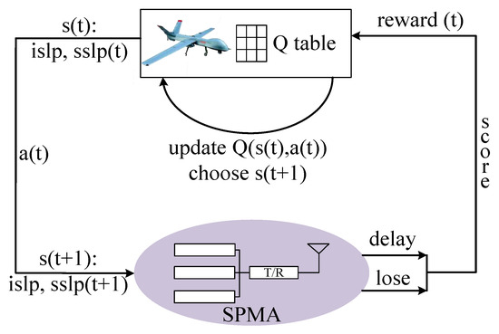
Figure 3. Q-learning for SPMA.

Algorithm 4 shows how Q-learning works in ACBS-RL to adjust the CBS parameters dynamically in the packet transmission. The inputs are the action a, $islp$, $sslp$, $isl{p}^{\prime }$, and $ssl{p}^{\prime }$. The output is the updated Q table. In line 3–5, the current $islp$, $sslp$ are assigned to the current state $s\left(t\right)$ and the updated $isl{p}^{\prime }$, $ssl{p}^{\prime }$ are assigned to the next state $s(t+1)$. The $Dela{y}_i$ and $Los{s}_i$ of each queue are calculated by Equations (6) and (7) during a training epoch (line 6). In line 7, the $Delay$ and $Loss$ of the node are obtained by averaging all $Dela{y}_i$ and $Los{s}_i$. Then, through Equations (8)–(11), we get the final reward $r_t$ of the node (line 8–9). In line 10–13, we choose the maximum Q value that can be get from the state $s(t+1)$ and update value $Q\left(s\right(t),a)$ to realize the maintenance of the Q table. Finally, the adjustment of the CBS parameter is finished and the new $Q(s,a)$ is returned (line 14–15). The Q-learning function ends.

Finally, we analyze the time complexity of our proposed ACBS-RL. Since the ACBS-RL algorithm is based on the classic Q-learning algorithm, the total time complexity of the Q-learning algorithm is O(N), where N is the total iteration times of the algorithm. Generally speaking, the value of N is related to the following factors: the size of state space |S|, the size of action space |A|, and the efficiency of exploration strategy (such as $\epsilon$-greedy). When we apply the Q-learning-based algorithm to the on-board devices for UAV networks, we need to consider the algorithm’s energy efficiency. The energy consumption of Q-learning is mainly determined by computing and memory access. In the Q-learning algorithm, the complexity of the Q-table update is O(1), and the frequent float calculation for Q-table update consumes energy. On the other hand, the Q-learning algorithm needs to read or write the Q-table in memory, which consumes the storage energy. Our proposed ACBS-RL algorithm is based on the Q-learning classic algorithm, and the state space and action space are limited, which are both constrained by the Q-table. Thus, the ACBS-RL is an energy-efficient algorithm and suitable for on-board devices for UAV networks.

5. Simulation

In this section, we evaluate the ACBS-RL algorithm through computer simulations. We present our simulation settings first, then we show the simulation results of the ACBS-RL algorithm compared with traditional SPMA and an adaptation backoff algorithm-based SPMA (A-COP). Our simulation methods can be easily extended to larger-scale or 3D UAV network scenarios [21].

5.1. Simulation Setting

Platform: Our platform for evaluation is a Lenovo workstation carrying one Intel core i7-11800H CPU 2.30 GHz with Ubuntu 20.04 on VMware workstation.

Network Topology: We use a single-hop network to evaluate the performance of our ACBS-RL algorithm. The network topology is illustrated in Figure 4, which contains 13 nodes randomly distributed in the scenario area. The nodes are reachable by a single hop, and the MAC layer of all nodes in the entire network uses the SPMA protocol.

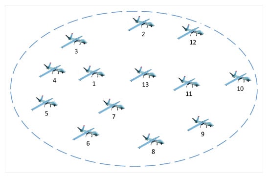
Figure 4. A UAV network topology with 13 nodes.

Parameters Setting: The parameters of SPMA is listed in Table 2. We calculate the highest priority threshold by continuously increasing the offered load until the success rate of packet arrival reaches 99% and the channel occupancy under this condition is selected as the highest priority threshold. The threshold for Priority 0, 1, 2 is set to 0.45, 0.24, 0.16. We set the learning rate $\alpha$ to 0.15 and the discount factor $\gamma$ to 0.1. And the weights $w_1$, $w_2$, and $w_3$ in the total score calculation are set to 0.5, 0.3, and 0.2. The number of training epochs is 200 in order to make the algorithm converge as much as possible. In the training environment, the packet arrival rate randomly switches between a Poisson distribution of rate of 10, 20, or 30 packets per millisecond and the ratio of three priorities varies randomly between 1:1:1 and 1:2:4.

Table 2. The parameters of SPMA.

Parameter Name	Parameter Value
Simulation time	100 s
Channel occupancy calculation window size	1 ms
Priority number of packets	3
Packet size	7200 bits
Transmission rate	40 Mbps
Number of orthogonal channels	5
Number of sub pulses per packet	27
Length of sub pulse	100 bits
Length of backoff window	1000 us
Duty cycle	15 %

The 200 training epochs in our simulation are primarily designed to ensure the convergence of the Q-learning model during offline pre-training, allowing the algorithm to learn robust adjustment strategies for CBS parameters (idleslope and sendslope) under diverse traffic patterns . For online deployment in dynamic UAV networks, we adopt a two-phase approach: offline pre-training with 200 epochs to initialize the Q-table, followed by lightweight online fine-tuning. Moreover, the Q-table update in ACBS-RL has a time complexity of O(1), and the lightweight characteristic of parameter adjustments (focused on idleslope and sendslope) ensures that each online iteration consumes minimal computational resources, aligning with the real-time requirements of UAV networks.

Comparing Benchmarks: We compare the following benchmarks with the proposed ACBS-RL.

• Baseline: The standard SPMA algorithm without any improvement.
• A-COP: The backoff time is adapted based on COS and priority in the method compared with SPMA.

Performance Metrics: We use the following four performance metrics to evaluate the effectiveness of our ACBS-RL algorithm.

• Network throughput: The total amount of data that passes through the UAV network. This is a metric used to measure the ability of processing data in a system.
• Packet loss rate: The ratio of packets lost with respect to packets sent in the system. It reflects the quality of transmission and we utilize this metric to evaluate the condition of a packet’s successful reception.
• Queuing delay: The time that a packet waits to be dequeued. This is a essential metric to qualify the algorithm performance in a given environment.
• Network scalability: We test the network performance under different numbers of network nodes to evaluate its scalability in dynamic UAV networks.

5.2. Results and Analysis

Network throughput: Figure 5a,b show the throughput of the network in two priority ratios (1:1:1 and 1:2:4). From Figure 5, we can see that the throughput of network in the three algorithms increases with the growth of offered load. Compared with SPMA and A-COP, the proposed ACBS-RL increases 14.48% and 11.61% throughput on average, respectively. This is because SPMA pays more attention to the transmission of highest priority packets. The lower priority packets are deprived of the transmission opportunity. In A-COP, the backoff time is dynamically adjusted based on COS and priority. However, the lower priority traffic are still preempted by the highest priority traffic. In ACBS-RL, the credit is always adjusted once the packets are transmitted. The lower priority packets obtain transmission opportunity even when there are some highest priority packets in the queue. It is observed that ACBS-RL efficiently makes full use of channel resources.

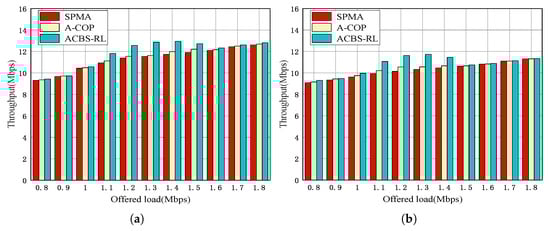
Figure 5. Throughput of the system in different priority ratios. (a) Priority ratio 1:1:1. (b) Priority ratio 1:2:4.

Packet loss rate: Figure 6a–c show the packet loss rate of the three priority packets in priority ratio 1:1:1. From Figure 6, we can see that the packet loss rate of all priority packets increases with the growth of offered load in three algorithms. Compared with SPMA and A-COP, the proposed ACBS-RL decreases the packet loss rate of Priority 2 packets by up to 58.21% and 47.24%, and the packet loss rate of Priority 1 packets by up to 10.11% and 8.57%. In addition, the packet loss rate of Priority 0 packets is still less than 1%. This is because SPMA and A-COP utilize strict priority-based queuing to control packet transmission. Even with the backoff mechanism, lower priority services are discarded because of waiting in the queue for too long under channel congestion. This results in packet loss. In ACBS-RL, the lower priority packets are transmitted when the credit is the highest in any condition. To a certain extent, ACBS-RL reduces the possibility of the lowest packets dropped due to waiting in the queue too long.

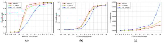
Figure 6. Packet loss rate in priority ratio 1:1:1. (a) Priority 2. (b) Priority 1. (c) Priority 0.

Figure 7a–c show the packet loss rate of the three priority packets in priority ratio 1:2:4. From Figure 7, we can see that the packet loss rate of all priority packets increases with the growth of offered load in three algorithms. Compared with SPMA and A-COP, the proposed ACBS-RL decreases the packet loss rate of Priority 2 packets by up to 28.73% and 18.12%. The packet loss rate of Priority 1 packets in ACBS-RL is not reduced too much. And the packet loss rate of Priority 0 packets is still less than 1%. This is because there are more lower priority packets in priority ratio 1:2:4 and the lowest priority packets obtain more transmission opportunities. In ACBS-RL, the Priority 0 and 1 both make efforts to reduce the packet loss rate of the lowest priority packets compared with SPMA and A-COP.

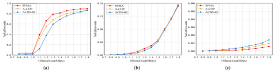
Figure 7. Packet loss rate in priority ratio 1:2:4. (a) Priority 2. (b) Priority 1. (c) Priority 0.

Queuing delay: Figure 8a–c show the queuing delay of the three priority packets in priority ratio 1:1:1. From Figure 8, we can see that the queuing delay of all priority packets increases with the growth of offered load in three algorithms. Compared with SPMA and A-COP, the proposed ACBS-RL decreases the queuing delay of Priority 2 packets by up to 4.62 ms and 2.58 ms. The queuing delay of Priority 1 packets is increased 1.12 ms and 0.57 ms and the queuing delay of Priority 0 packets is increased 400 us and 160 us compared with SPMA and A-COP in priority ratio 1:1:1. This is because in SPMA, the lowest priority packets are dequeued when the COS meet the requirement of the queue. In A-COP, the backoff time of packets is suitable for COS and priority. However, the packets undergo repeated backoffs when there are high channel load conditions. This significantly increases queuing delays due to prolonged contention for channel access. In ACBS-RL, the lowest priority packets are given more opportunities to check the COS requirement for transmission and the highest priority packets mainly give the resource to the lower priority packets.

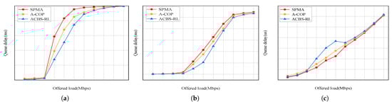
Figure 8. Queue delay in priority ratio 1:1:1. (a) Priority 2. (b) Priority 1. (c) Priority 0.

Figure 9a–c show the queuing delay of the three priority packets in priority ratio 1:2:4. From Figure 9, we can see that the queuing delay of all priority packets increases with the growth of offered load in three algorithms. Compared with SPMA and A-COP, the proposed ACBS-RL decreases the queuing delay of Priority 2 packets by up to 2.51 ms and 1.68 ms. The queuing delay of Priority 1 packets is increased by 100 ms and 60 ms and the queuing delay of Priority 0 packets is increased by 200 us and 120 us compared with SPMA and A-COP in priority ratio 1:2:4. In ACBS-RL, the packets except for the lowest priority both provide the resource to the lowest priority packets in this scenario. The queuing delay of the highest priority packets increases a bit because there are some resources which are not used for transmission. ACBS-RL utilizes the spare resources fully and does not influence the queuing delay of the highest priority packets. From the above simulation results, the performance of high-priority packets is not compromised in our proposed ACBS-RL. However, in the condition of a very high traffic load, the performance of high-priority packets is adversely impacted, especially in the terms of queue delay and packet loss. The reason is that when traffic load is very high, the high-priority queue needs to adaptively transfer more transmission chances to the lower-priority queue according to our proposed ACBS-RL algorithm. On the other hand, for some mission-critical applications in UAV networks, the increase of delay for high-priority packets may violate the QoS requirement. To solve this problem, we can adjust the key parameters in our algorithm (such as idleslope and sendslope in CBS) to guarantee the QoS constraint.

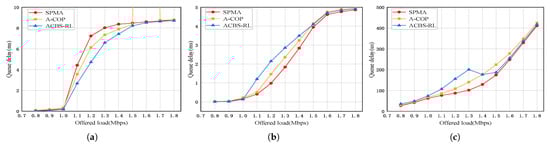
Figure 9. Queue delay in priority ratio 1:2:4. (a) Priority 2. (b) Priority 1. (c) Priority 0.

Network scalability: Figure 10a–c show the network performance of 20 nodes in priority ratio 1:1:1. Figure 11a–c show the network performance of 30 nodes in priority ratio 1:1:1. From Figure 10a and Figure 11a, we can see that the throughput at different numbers of nodes shows specific trends. With 13 nodes, total network throughput ranges from 9.4 Mbps to 12.8 Mbps. With 20 nodes, throughput slightly decreases to 9.2 Mbps to 12.4 Mbps. With 30 nodes, it further drops to 9.0 Mbps to 12.1 Mbps. This trend indicates that increasing node count intensifies channel contention. More nodes competing for limited resources lead to increased collisions and backoff times. ACBS-RL mitigates such issues by dynamically adjusting credits and parameters to better utilize channel resources. However, it cannot fully offset the negative impact of intensified contention, resulting in gradual throughput decrease with more nodes.

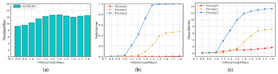
Figure 10. Network performance of 20 nodes in priority ratio 1:1:1. (a) Throughput. (b) Packet loss rate. (c) Queue delay.

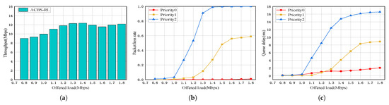
Figure 11. Network performance of 30 nodes in priority ratio 1:1:1. (a) Throughput. (b) Packet loss rate. (c) Queue delay.

Figure 10b and Figure 11b show the packet loss rate at different numbers of nodes. Packet loss rate exhibits a clear upward trend with increasing node counts. With 13 nodes, packet loss rates of Priority 2 packet reach up to 0.95 under high load. With 20 nodes, this increases to near 0.99. And at 30 nodes, it approaches 1.0. This trend stems from intensified channel contention. More nodes generate heavier traffic, elevating collision risks and prolonging queue waiting times. Low-priority packets suffer most, as they are more likely to exceed timeout thresholds during extended waiting. ACBS-RL mitigates this by dynamically adjusting CBS parameters via Q-learning. It allocates transmission opportunities based on credit values, ensuring low-priority queues gain access even under high load. However, its effectiveness is limited. With excessive nodes, channel resources are overcommitted, and credit-based scheduling cannot fully prevent losses caused by timeouts.

Figure 10c and Figure 11c show the queue delay at different numbers of nodes. With escalating node counts, the queue delay of the Priority 0 packet exhibits a consistent upward trajectory: from 64–1235 us at 13 nodes, escalating to 85–1647 us at 20 nodes, and peaking at 107–2059 us at 30 nodes. More nodes intensify channel contention, increasing collisions and backoff times. Though ACBS-RL mitigates queue delay via the dynamic adjustment of CBS parameters, it fails to completely offset contention-driven latency growth.

6. Conclusions and Future Works

In this paper, we propose the method of ACBS-RL with reinforcement learning to balance the performance of all-priority traffic for SPMA in UAV networks. The CBS is utilized to provide relatively fair packet transmission opportunity among multiple traffic queues by limiting the transmission rate. To face the dynamic situations of UAV networks, the Q-learning is leveraged to adaptively adjust the parameters of CBS to achieve better performance among all priority queues. The extensive simulation results show that the ACBS-RL can increase network throughput while guaranteeing QoS requirements of all priority traffic. Our future work will explore the application of machine learning methods (such as deep neural networks) on SPMA protocol design for UAV networks, which can adaptively adjust the key parameters (such as backoff time, COS, SSW, etc.) in dynamic and complicated environments.

References

- Zhang, X.; Zhang, H.; Sun, K.; Long, K.; Li, Y. Human-centric irregular RIS-assisted multi-UAV networks with resource allocation and reflecting design for metaverse. IEEE J. Sel. Areas Commun. 2024, 42, 603–615. [Google Scholar] [CrossRef]
- Liu, Y.; Xie, J.; Xing, C.; Xie, S.; Luo, X. Self-organization of UAV networks for maximizing minimum throughput of ground users. IEEE Trans. Veh. Technol. 2024, 73, 11743–11755. [Google Scholar] [CrossRef]
- Wu, J.; Zhou, J.; Yu, L.; Gao, L. MAC optimization protocol for cooperative UAV based on dual perception of energy consumption and channel gain. IEEE Trans. Mob. Comput. 2024, 23, 9851–9862. [Google Scholar] [CrossRef]
- Mao, K.; Zhu, Q.; Wang, C.; Ye, X.; Gomez-Ponce, J.; Cai, X.; Miao, Y.; Cui, Z.; Wu, Q.; Fan, W. A survey on channel sounding technologies and measurements for UAV-assisted communications. IEEE Trans. Instrum. Meas. 2024, 73, 8004624. [Google Scholar] [CrossRef]
- Touati, H.; Chriki, A.; Snoussi, H.; Kamoun, F. Cognitive radio and dynamic TDMA for efficient UAVs swarm communications. Comput. Netw. 2021, 196, 108264. [Google Scholar] [CrossRef]
- Chen, J.; Wang, J.; Wang, J.; Bai, L. Joint fairness and efficiency optimization for CSMA/CA-based multi-user MIMO UAV ad hoc networks. IEEE J. Sel. Top. Signal Process. 2024, 18, 1311–1323. [Google Scholar] [CrossRef]
- Ripplinger, D.; Narula-Tam, A.; Szeto, K. Scheduling vs. random access in frequency hopped airborne networks. In Proceedings of the IEEE Military Communications Conference (MILCOM), Orlando, FL, USA, 29 October–1 November 2012. [Google Scholar]
- Liu, J.; Peng, T.; Quan, Q.; Cao, L. Performance analysis of the statistical priority-based multiple access. In Proceedings of the IEEE International Conference on Computer and Communications (ICCC), Chengdu, China, 13–16 December 2017. [Google Scholar]
- Zheng, W.; Jin, H. Analysis and research on a new data link MAC protocol. In Proceedings of the IEEE International Conference on Communication Software and Networks (ICCSN), Chengdu, China, 6–9 July 2018. [Google Scholar]
- Wang, L.; Li, H.; Liu, Z. Research and pragmatic-improvement of statistical priority-based multiple access protocol. In Proceedings of the IEEE International Conference on Computer and Communications (ICCC), Chengdu, China, 14–17 October 2016. [Google Scholar]
- Zhang, Y.; Sun, H.; He, Y.; Zhang, Z.; Wang, X.; Quek, T.Q.S. A spatio-temporal analytical model for statistical priority-based multiple access network. IEEE Wirel. Commun. Lett. 2023, 12, 153–157. [Google Scholar] [CrossRef]
- Gao, S.; Yang, M.; Yu, H. Modeling and parameter optimization of statistical priority-based multiple access protocol. China Commun. 2019, 16, 45–61. [Google Scholar] [CrossRef]
- Liu, P.; Wang, C.; Lei, M.; Li, M.; Zhao, M. Adaptive priority-threshold setting strategy for statistical priority-based multiple access network. In Proceedings of the IEEE Vehicular Technology Conference (VTC), Antwerp, Belgium, 25–28 May 2020. [Google Scholar]
- Zhang, Y.; He, Y.; Sun, H.; Wang, X.; Quek, T.Q.S. Performance analysis of statistical priority-based multiple access network with directional antennas. IEEE Wirel. Commun. Lett. 2022, 11, 220–224. [Google Scholar] [CrossRef]
- Zhang, Y.; He, Y.; Wang, X.; Sun, H.; Quek, T.Q.S. Modeling and performance analysis of statistical priority-based multiple access: A stochastic geometry approach. IEEE Internet Things J. 2022, 9, 13942–13954. [Google Scholar] [CrossRef]
- He, S.; An, Z.; Zhu, J.; Zhang, M.; Huang, Y. Cross-layer optimization: Joint user scheduling and beamforming design with QoS support in joint transmission networks. IEEE Trans. Commun. 2023, 71, 792–807. [Google Scholar] [CrossRef]
- Wang, S.; Liu, H.; Gomes, P.H.; Krishnamachari, B. Deep reinforcement learning for dynamic multichannel access in wireless networks. IEEE Trans. Cogn. Commun. Netw. 2018, 4, 257–265. [Google Scholar] [CrossRef]
- Chen, X.; Huang, C.; Fan, X.; Liu, D.; Li, P. LDMAC: A propagation delay-aware MAC scheme for long-distance UAV networks. Comput. Netw. 2018, 144, 40–52. [Google Scholar] [CrossRef]
- Feng, P.; Bai, Y.; Huang, J.; Wang, W.; Gu, Y.; Liu, S. CogMOR-MAC: A cognitive multi-channel opportunistic reservation MAC for multi-UAVs ad hoc networks. Comput. Commun. 2019, 136, 30–42. [Google Scholar] [CrossRef]
- Li, B.; Guo, X.; Zhang, R.; Du, X. Performance analysis and optimization for the MAC protocol in UAV-based IoT network. IEEE Trans. Veh. Technol. 2020, 69, 8925–8937. [Google Scholar] [CrossRef]
- Wang, J.; Zhu, Q.; Lin, Z.; Chen, J.; Ding, G.; Wu, Q.; Gu, G.; Gao, Q. Sparse bayesian learning-based hierarchical construction for 3D radio environment maps incorporating channel shadowing. IEEE Trans. Wirel. Commun. 2024, 23, 14560–14574. [Google Scholar] [CrossRef]
Disclaimer/Publisher’s Note: The statements, opinions and data contained in all publications are solely those of the individual author(s) and contributor(s) and not of MDPI and/or the editor(s). MDPI and/or the editor(s) disclaim responsibility for any injury to people or property resulting from any ideas, methods, instructions or products referred to in the content. |
© 2025 by the authors. Licensee MDPI, Basel, Switzerland. This article is an open access article distributed under the terms and conditions of the Creative Commons Attribution (CC BY) license (https://creativecommons.org/licenses/by/4.0/).