Accurate Tracking of Agile Trajectories for a Tail-Sitter UAV Under Wind Disturbances Environments

Abstract

To achieve more robust and accurate tracking control of high maneuvering trajectories for a tail-sitter fixed-wing unmanned aerial vehicle (UAV) operating within its full envelope in outdoor environments, a novel control approach is proposed. Firstly, the study rigorously demonstrates the differential flatness property of tail-sitter fixed-wing UAV dynamics using a comprehensive aerodynamics model, which incorporates wind effects without simplification. Then, utilizing the derived flatness functions and the treatments for singularity, the study presents a complete process of the differential flatness transform. This transformation maps the desired maneuver trajectory to a state-input trajectory, facilitating control design. Leveraging an existing controller from the reference literature, trajectory tracking is implemented. Subsequently, a low-cost wind estimation method operating during all flight phases is proposed to estimate the wind effects involved in the model. The wind estimation method involves generating a virtual wind measurement utilizing a low-fidelity tail-sitter model. The virtual wind measurement is integrated with real wind data obtained from the pitot tube and processed through fusion using an extended Kalman filter. Finally, the effectiveness of our methods is confirmed through comprehensive real-world experiments conducted in outdoor settings. The results demonstrate superior robustness and accuracy in controlling challenging agile maneuvering trajectories compared to the existing method. Additionally, the test results highlight the effectiveness of our method in wind estimation.

1. Introduction

Accompanied by the great breakthroughs in the fields of perceptual technology, computing, and sensor miniaturization, unmanned aerial vehicles (UAVs) with advanced capabilities are developing fast. The tail-sitter fixed-wing UAV is a remarkable UAV designed for versatile aerial operations. Compared to other vertical takeoff and landing (VTOL) fixed-wing UAVs, such as dual-systems [1,2], tilt-wings [3], and tilt-rotors [4], the tail-sitter fixed-wing UAV boasts a significant advantage due to its lack of dedicated control surfaces, such as ailerons, elevators, and rudders. Instead, it relies on a sophisticated system of actuators that remain active throughout all flight phases. This design feature eliminates the need for heavy and complex mechanisms associated with transitioning between vertical and horizontal flight modes [1], thereby sparking considerable research interest and fostering the development of diverse tail-sitter fixed-wing UAVs [5,6,7]. One such vehicle is the tail-sitter flying-wing UAV, which lacks vertical control surfaces [8]. This design makes it easier to execute aggressive maneuvers. Research on agile maneuverability flight control for the tail-sitter flying-wing UAV is crucial due to its inherent high maneuverability, which holds immense potential for addressing diverse challenging missions. These missions encompass emergency responses and navigating swiftly through obstacle- laden environments.

Currently, the field of agile maneuver flight control under the full envelope of tail-sitter flying-wing UAVs is in its nascent stages, with a noticeable scarcity of related technologies. To date, the team led by Tal et al. stands as the sole contributor to advancements within this specialized area. In 2023, Tal et al. introduced an algorithm for agile trajectory generation tailored to a tail-sitter flying-wing UAV, representing a pioneering effort in this domain [9]. This algorithm leverages the differential flatness of a realistic tail-sitter UAV flight dynamics model to generate agile flight trajectories. Additionally, the computational and experimental results presented in [9] validate the suitability of the derived flatness transform for assessing the dynamic feasibility of candidate trajectories. Shortly thereafter, Tal et al. proposed a novel global controller designed for accurate tracking of these agile trajectories using a tail-sitter flying-wing UAV [8]. Unlike previous approaches reliant on extensive aerodynamic modeling, this global controller utilizes incremental nonlinear dynamic inversion (INDI) to compute control updates, enabling maneuvering across the flight envelope.

While Tal et al. [8,9] have conducted extensive indoor real-flight tests to validate the efficacy of their methods in tracking agile trajectories, a notable challenge persists in outdoor flight conditions. This challenge revolves around the differential flatness analysis of tail-sitter flying-wing UAV dynamics. As outlined in [9], these vehicles represent under-actuated systems with highly nonlinear aerodynamics. Unlike traditional fixed-wing UAVs, which typically operate within a conservative flight regime characterized by linear aerodynamics, tail-sitter UAVs traverse a broad flight envelope with varying angles of attack (AOA), leading to extreme nonlinearities in wing aerodynamics. Consequently, the exploration of the differential flatness of tail-sitter flying-wing UAV dynamics, leveraging comprehensive aerodynamic models, poses significant complexities and remains an open question. In an effort to mitigate this complexity, Tal et al. [9] employed a coarse $\varphi$-theory [10] to construct the aerodynamic model. However, this simplified model disregards wind effects, consequently neglecting crucial aerodynamic angles like the AOA and sideslip angle. Consequently, the derived differential flatness may compromise trajectory quality and resultant control performance. While Tal et al. [9] utilized incremental control to partially counteract the resultant unmodeled forces and moments, integrating wind considerations into the control design could further enhance performance [11].

Therefore, this article is primarily dedicated to tackling the unresolved challenge outlined in references [8,9]. In tackling this challenge, we opt for the utilization of a comprehensive aerodynamic model that incorporates wind effects without any simplifications [12]. Leveraging this accurate model, intricate theoretical analyses are conducted to establish the differential flatness property. Additionally, we derive novel differential flatness transform functions, which are instrumental in converting agile trajectory targets into corresponding state and feedforward control input trajectories. The incorporation of wind effects during trajectory transformation enables preemptive compensation for wind disturbances, thereby mitigating the accumulation of control errors. As the primary emphasis of this paper lies outside the realm of trajectory tracking controller design, we resort to employing existing controllers documented in reference [9] to track the state trajectories generated through the derived differential flatness transform functions.

To address wind effects in the model, conventional instruments such as vane-type flow angle sensors can be employed for wind estimation. However, these instruments are complex and are typically reserved for large vehicles, such as commercial or research planes, owing to their associated payload and cost. In contrast, low-cost UAVs usually lack such instrumentation. Hence, there arises a critical need to devise a viable, cost-effective, and precise method for wind estimation tailored to small UAVs.

The prevailing wind estimation methodologies for small UAVs in the literature primarily pertain to conventional fixed-wing UAVs and can be categorized into two primary categories. The first category involves utilizing the “wind triangle” which denotes the mathematical relationship among the wind speed, ground speed, and airspeed. This method, widely adopted due to its simplicity, does not explicitly consider the UAV’s dynamic model. For instance, Petrich et al. [13] proposed a method to estimate the 3-D wind components by integrating measurements from an airspeed sensor, a compass, an IMU, and a GPS, utilizing a Kalman filter for data fusion. Similarly, Langelaan et al. [14] incorporated the wind gradient and vehicle acceleration into their wind estimation algorithm for miniature UAVs. They also underscored the relationship between wind velocity accuracy and the vehicle’s airspeed and orientation. Additionally, Kim et al. [15] introduced an estimation method working in constant wind conditions, which employs data from a pitot tube and a GPS. The nonlinear observation function in their method is managed using an extended Kalman filter (EKF). However, their approach requires variation in the UAV’s heading to determine the wind direction. Another category estimates wind effects utilizing the vehicle’s dynamics model [15,16,17]. For example, Divitiis et al. [18] deemed it impractical to install wind speed measuring instruments on rotorcraft due to potential biases from rotor flow. Consequently, they devised a wind estimation method grounded in aerodynamic models. The principle underlying this method is that wind alters the UAV’s motion state, encompassing speed and direction. By solving the motion equations and integrating aerodynamic models, the effect of this wind can be inferred. Their experimental findings indicate that the wind estimation method based on aerodynamic models converges faster and provides more accurate estimates compared to the wind triangle method. However, this approach entails using neural networks to estimate the UAV’s aerodynamic coefficients, presenting significant deployment challenges.

Compared to conventional fixed-wing UAVs, designing a reliable and effective approach employed on the tail-sitter flying-wing UAVs for wind estimation poses significant challenges, primarily due to its broad flight envelope. While an airspeed sensor can measure airspeed during cruising, its effectiveness diminishes during hovering phases. In such instances, particularly during takeoff or landing phases, the airspeed sensor may only capture a partial aspect of the incoming flow velocity, or in some cases, no data at all. A notable study addressing wind estimation for tail-sitter flying-wing UAVs is presented in [19]. This research initially established the relationship between ground speed and vehicle attitude through parameter identification. Subsequently, it utilized this attitude-velocity relationship and the “wind triangle” concept to calculate the wind speed. However, it is essential to note that this paper [19] primarily studied the hovering stage where the pitch angle has a fixed range. Consequently, data beyond this range could not be reliably inferred. While the developed method shows promise for the hovering stage, its direct extension to cover the entire flight envelope remains challenging.

Drawing inspiration from the literature above, we propose leveraging the dynamic model of the tail-sitter flying-wing UAV to obtain a virtual wind measurement. This virtual wind information operates independently of the conventional pitot tube. In essence, this approach involves equipping the vehicle with two sensors: one that provides higher accuracy during cruising (the pitot tube), and another that is particularly effective during hovering (the virtual wind measurement). For integrating these measurements, we consider the sensor fusion architecture, EKF. It is worth noting that previous studies [20] have indicated challenges when using Kalman filters to fuse data from low-cost sensors, potentially leading to suboptimal outcomes. Nonetheless, Kalman filters remain widely employed and effective for data fusion tasks, particularly in scenarios involving measurement noise and model uncertainty. The crucial aspect is to carefully select filter configurations and adjust parameters based on specific application contexts and system requirements, ensuring alignment with performance and accuracy criteria.

In short, this study addresses the challenge of achieving robust and accurate agile maneuver tracking control for a tail-sitter flying-wing UAV under full envelope in outdoor wind conditions. It does so by utilizing a comprehensive aerodynamic model that incorporates wind effects without any simplification. The contributions are delineated as follows:

• This study showcases the differential flatness property of a tail-sitter flying-wing UAV through an intricate and thorough theoretical examination. New flatness functions are deduced. In contrast to existing analytical approaches employing a simplified aerodynamics model, our method relies on a comprehensive aerodynamic model that encompasses wind effects without any simplification. By integrating wind effects into the flatness functions, it becomes possible to preemptively compensate for the impact of wind before control errors accumulate.
• Based on the derived flatness functions and the treatments for singularity, this study presents a complete process of the differential flatness transform, which maps the desired maneuver trajectory to a state-input trajectory.
• Concerning the inclusion of wind effects in the model, this study introduces a novel, cost-effective, and precise wind estimation approach. The method involves proposing a virtual wind measurement derived from a low-fidelity tail-sitter UAV model. The virtual wind measurement is integrated with real wind data obtained from the pitot tube and processed through fusion using an EKF. Notably, our approach stands out by its applicability to all flight phases of the tail-sitter flying-wing UAV, distinguishing it from existing methods documented in the literature.
• Our methods’ effectiveness is validated through thorough real-world flight tests in outdoor environments. It is worth noting that previous literature seldom showcases real-world agile flights in windy outdoor conditions. The outcomes illustrate superior robustness and accuracy in controlling demanding agile maneuvering trajectories compared to established methods. Moreover, the test results underscore the efficacy of our wind estimation approach.

This paper’s structure is delineated as follows: Section 2 specifies the system model. The proposed method for wind estimation is elaborated upon in Section 3. Section 4 shows how the differential flatness is derived and presents the complete differential flatness transform. Section 5 outlines the proposed control architecture. Real-world experiments validating our approach are detailed in Section 6. Finally, Section 7 encapsulates this paper’s conclusions.

2. System Modeling

The coordinate frames of a tail-sitter flying-wing UAV are defined following the conventional setup of fixed-wing UAVs (see Figure 1). The earth-fixed frame $\left({\mathit{x}}_I,{\mathit{y}}_I,{\mathit{z}}_I\right)$ adheres to the north–east–down (NED) convention. The body-fixed frame $\left({\mathit{x}}_B,{\mathit{y}}_B,{\mathit{z}}_B\right)$ is oriented as forward–right–down. Notably, the axes of the rotor-fixed frame $\left({\mathit{x}}_P,{\mathit{y}}_P,{\mathit{z}}_P\right)$ align parallel to those of the body-fixed frame.

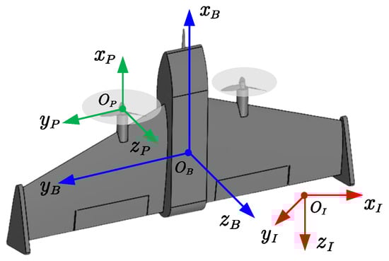
Figure 1. The coordinate frames of a tail-sitter flying-wing UAV.

The translational and rotational dynamics of the tail-sitter flying-wing UAV are described using the Newton–Euler equations:

$$\left\{\begin{array}{c}\dot{\mathit{P}}={\mathit{V}}_g^I\hfill \\ m{\dot{\mathit{V}}}_g^I=m\mathit{g}+m{a}_T{\mathit{R}}_B^I{\mathit{e}}_1+{\mathit{R}}_B^I{\mathit{F}}_a\hfill \\ {\dot{\mathit{R}}}_B^I={\mathit{R}}_B^I⟨\mathit{\omega }⟩\hfill \\ \mathit{J}\dot{\mathit{\omega }}=\mathit{\tau }+{\mathit{M}}_a-\mathit{\omega }\times \mathit{J}\mathit{\omega }\hfill \end{array}\right.,$$

(1)

where ${\mathit{V}}_g^I$ represents the velocity; $\mathit{P}$ denotes the position; ${\mathit{F}}_a$ and ${\mathit{M}}_a$ represent the aerodynamic force and moment, respectively; $\mathit{\omega }$ represents the angular velocity; $\mathit{g}$ stands for gravitational acceleration; m represents vehicle mass; ${\mathit{R}}_B^I$ is the rotation matrix; $\mathit{J}$ is the inertia matrix; $a_T$ indicates the thrust acceleration, and $\mathit{\tau }$ denotes the control moment; $⟨\mathit{a}⟩$ represents a notation which converts a vector into a skew-symmetric matrix; ${\mathit{e}}_1={\left[\begin{array}{ccc}1& 0& 0\end{array}\right]}^{\mathrm{T}}$. The input and state vectors of the system are defined as:

$$\left\{\begin{array}{c}{\mathit{U}}_{full}=\left(a_T,\mathit{\tau }\right)\hfill \\ {\mathit{X}}_{full}=\left(\mathit{P},{\mathit{V}}_g^I,{\mathit{R}}_B^I,\mathit{\omega }\right)\hfill \end{array}\right..$$

(2)

Referring to [21], ${\mathit{F}}_a$ and ${\mathit{M}}_a$ can be modeled as follows:

$$\left\{\begin{array}{c}{\mathit{F}}_a=\left[\begin{array}{c}{F}_{a_x}\\ F_{a_y}\\ F_{a_z}\end{array}\right]=\left[\begin{array}{ccc}-cos\alpha & 0& sin\alpha \\ 0& 1& 0\\ -sin\alpha & 0& -cos\alpha \end{array}\right]\left[\begin{array}{c}D\\ Y\\ \Gamma \end{array}\right]\hfill \\ {\mathit{M}}_a={\left[\begin{array}{ccc}L& M& N\end{array}\right]}^{\mathrm{T}}\hfill \end{array}\right.,$$

(3)

where $\alpha$ is the AOA. $\Gamma$, D, and Y are the lift, drag, and side force, respectively. L, M, and N are the rolling, pitching, and yawing moment, respectively. These force and moment components can be expressed as products involving mean aerodynamic chord $\overline{c}$, wing area S, dynamic pressure, and aerodynamic coefficients:

$$\left[\begin{array}{c}D\\ Y\\ \Gamma \end{array}\right]=\left[\begin{array}{c}{\displaystyle \frac{1}{2}}\rho V^{2}S{C}_D\\ {\displaystyle \frac{1}{2}}\rho V^{2}S{C}_Y\\ {\displaystyle \frac{1}{2}}\rho V^{2}S{C}_{\Gamma }\end{array}\right],\left[\begin{array}{c}L\\ M\\ N\end{array}\right]=\left[\begin{array}{c}{\displaystyle \frac{1}{2}}\rho V^{2}S\overline{c}{C}_L\\ {\displaystyle \frac{1}{2}}\rho V^{2}S\overline{c}{C}_M\\ {\displaystyle \frac{1}{2}}\rho V^{2}S{C}_N\end{array}\right],$$

(4)

where $V=∥{\mathit{V}}_a∥$ represents the magnitude of airspeed; $\rho$ denotes the air density; $C_{\ast }\left(\ast =\Gamma ,D,Y,L,M,N\right)$ are the aerodynamic coefficients which are functions of the AOA $\alpha$, the sideslip angle $\beta$, the Reynolds number $Re$, and the deflection angles of the control surfaces ${\delta }_{cs}$. Our previous work [22] has identified there coefficients through wind tunnel tests.

The airspeed ${\mathit{V}}_a^I$, AOA $\alpha$, and sideslip angle $\beta$ can be obtained using

$$\left\{\begin{array}{c}{\mathit{V}}_a^I={\mathit{V}}_g^I-{\mathit{V}}_w^I\hfill \\ {\mathit{V}}_a^B={\left({\mathit{R}}_B^I\right)}^{\mathrm{T}}{\mathit{V}}_a^I+{\mathit{V}}_{pro}^B=\left[\begin{array}{ccc}{V}_{a_x}^B& V_{a_y}^B& V_{a_z}^B\end{array}\right]\hfill \\ \alpha ={tan}^{-1}\left(V_{a_z}^B/V_{a_x}^B\right)\hfill \\ \beta ={tan}^{-1}\left(V_{a_y}^B/V_{a_x}^B\right)\hfill \end{array}\right.,$$

(5)

where ${\mathit{V}}_g^I$ is the ground velocity; ${\mathit{V}}_W^I$ is the wind speed; ${\mathit{V}}_{pro}^B$ is the propeller slipstream speed [23]; ${\mathit{V}}_a^B$ is the airspeed defined in the body-fixed frame.

Remark 1. 

The UAV model constructed in this paper incorporates wind, a significant deviation from the approach outlined in [8]. Thus, the presented UAV model offers enhanced realism and better alignment with practical scenarios. Section 3 will elaborate on the algorithm for wind estimation.

3. Wind Estimation Method for Tail-Sitter UAV

3.1. Wind Estimation Architecture

To address the constraint on sensor bias and wind states, we propose a cascaded estimation architecture for the tail-sitter flying-wing UAV (see Figure 2). This architecture comprises three sequential steps. Initially, the estimation process focuses on determining the vehicle’s attitude, ground speed, and position through a vehicle estimator, which integrates data from the compass, GPS, barometer, and IMU. Next, the aerodynamic model leverages the outcomes from the initial estimator to simulate a virtual wind measurement. Finally, the wind estimator generates the estimated wind state by fusing this virtual wind measurement with data from the pitot tube. Note that the ground speed and attitude data obtained from the vehicle state estimator contribute to the time-update equations within the wind estimator. The designed architecture can mitigate the potential corruption of state estimation by dynamic model errors by employing distinct estimators to manage the wind estimation problem and the vehicle’s states separately.

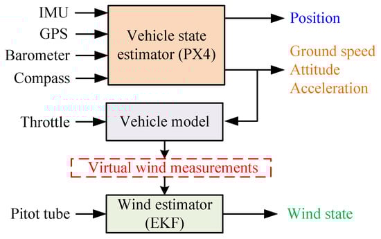
Figure 2. Cascaded wind estimator structure for the tail-sitter flying-wing UAV.

As shown in Figure 2 of the manuscript, the structure of the proposed wind estimation method involves the aircraft model generating a virtual wind estimate, which is then fused with the pitot tube measurement using EKF to yield the final wind estimate. Therefore, the process does not involve switching between different wind estimation methods, but rather continuous data fusion and correction by both methods throughout the entire flight.

The main focus of this paper is the development of a wind estimator tailored specifically for a tail-sitter flying-wing UAV, rather than the vehicle state estimator. Consequently, we adopt the state estimator available in the open-source PX4 firmware. It is worth noting that this study primarily focuses on horizontal wind, which can be characterized as a first-order Markov process [24]. Consequently, the wind speed vector ${\mathit{V}}_W^I$, assuming horizontal motion, is represented as ${\mathit{W}}^I=\left[\begin{array}{ccc}{W}_N& W_E& 0\end{array}\right]$, where $W_N$ and $W_E$ denote the north and east components. Virtual wind measurements of $W_N$ and $W_E$ are denoted as ${\left[\begin{array}{cc}{W}_N^S& W_E^S\end{array}\right]}^{\mathrm{T}}$. We define $v_W$ as the magnitude of ${\mathit{W}}^I$, and define ${\Phi }_W$ as the wind direction (the angle between the wind vector and the north direction), therefore, the wind parameters that need to be estimated include $v_W$ and ${\Phi }_W$.

Remark 2. 

The assumption of uniform wind fields used in this study is primarily due to the specific conditions of the small tail-sitter flying-wing UAV. This UAV operates within a limited flight range (less than 2 km), at relatively low altitudes (below 100 m), and for short durations (less than 15 min). Under these conditions, the wind field is generally simple, dominated by horizontal winds. Therefore, assuming uniform wind fields is reasonable in this context, which is also a common assumption in similar studies. Additionally, adopting this assumption significantly improves the computational efficiency of the wind estimation algorithm, which is crucial for real-time deployment and application in practical flight scenarios.

Here, ${\mathit{x}}_W={\left[\begin{array}{cc}{v}_W& {\Phi }_W\end{array}\right]}^{\mathrm{T}}$ is used to represent the wind state vector. It can be constructed as a random-walk process where the state transition functions are expressed as:

$${\mathit{x}}_W\left(k+1\right)={\mathit{Ax}}_W\left(k\right)+{\mathit{w}}_k.$$

(6)

In Equation (6), $\mathit{A}$ represents a second-order identity matrix; ${\mathit{w}}_k$ is the random noise. We define the measurement as ${\mathit{z}}_W\left(k\right)={\left[\begin{array}{ccc}{Q}_{pit}& W_N^S& W_E^S\end{array}\right]}^{\mathrm{T}}$, where $Q_{pit}$ is the dynamic pressure and can be directly obtained from a pitot tube. Thus, the nonlinear observation system can be constructed as

$${\mathit{z}}_W\left(k\right)={\mathit{Hx}}_W+{\mathit{v}}_k,$$

(7)

where $\mathit{H}$ represents the Jacobian matrix derived from the observation functions $\mathit{h}\left({\mathit{x}}_W\right)$. $\mathit{h}\left({\mathit{x}}_W\right)$ consists of the virtual wind measurement ${\mathit{h}}_s\left({\mathit{x}}_W\right)$ and the observation functions of the pitot tube $h_p\left({\mathit{x}}_W\right)$, that is

$$\mathit{h}\left({\mathit{x}}_W\right)=\left[\begin{array}{c}{h}_p\left({\mathit{x}}_W\right)\\ {\mathit{h}}_s\left({\mathit{x}}_W\right)\end{array}\right].$$

(8)

In Equation (7), ${\mathit{v}}_k$ is the measurement noise.

3.2. Virtual Wind Measurements

Virtual wind measurements are obtained by evaluating two expressions of ${\mathit{F}}_a$, that is ${\mathit{F}}_{a1}$ and ${\mathit{F}}_{a2}$. Specifically, by making ${\mathit{F}}_{a1}$ and ${\mathit{F}}_{a2}$ equal, the virtual wind measurement can be solved.

${\mathit{F}}_{a1}$ can be derived using the aerodynamic model in Section 2. For these aerodynamic coefficients, they can be expressed with:

$$\left\{\begin{array}{c}{C}_{\Gamma }={\mathcal{F}}_{\Gamma }\left(\alpha ,\beta ,Re,{\delta }_{cs}\right)\hfill \\ C_D={\mathcal{F}}_D\left(\alpha ,\beta ,Re,{\delta }_{cs}\right)\hfill \\ C_Y=\gamma \hfill \end{array}\right.,$$

(9)

where ${\mathcal{F}}_{\Gamma }$ and ${\mathcal{F}}_D$ are the nonlinear functions and can be obtained from the wind tunnel experiments. Note that $C_Y$ is treated as a constant since the slip angle $\beta$ is commonly assumed to be small. In this study, we disregard the variations in $C_{\Gamma }$ and $C_D$ due to the control surfaces deflection ${\delta }_{cs}$, as these surfaces primarily alter the moment coefficient. Additionally, the vehicle is designed to operate within a low Reynolds number regime, and its operation is confined to a narrow Reynolds number range. Consequently, the impact of $Re$ on $C_{\Gamma }$ and $C_D$ can be neglected. With these assumptions, Equation (9) can be rewritten as

$$\left\{\begin{array}{c}{C}_{\Gamma }={\mathcal{F}}_{\Gamma }\left(\alpha ,\beta \right)\hfill \\ C_D={\mathcal{F}}_D\left(\alpha ,\beta \right)\hfill \\ C_Y=\gamma \hfill \end{array}\right..$$

(10)

The rotation matrix

$${\mathit{R}}_I^B=\left[\begin{array}{ccc}{R}_{11}& R_{12}& R_{13}\\ R_{21}& R_{22}& R_{23}\\ R_{31}& R_{32}& R_{33}\end{array}\right]$$

can be updated using the vehicle state estimator in the wind estimation architecture. The ground speed in the body-fixed frame ${\mathit{V}}_g^B$ is denoted by ${\mathit{V}}_g^B={\left[\begin{array}{ccc}{V}_{g,x}^B& V_{g,y}^B& V_{g,z}^B\end{array}\right]}^{\mathrm{T}}$. For the sake of streamlining the estimation problem, we assume that the variance in rotation speed between the two propellers can be negligible. Consequently, ${\mathit{V}}_a^B$ can be rewritten as

$${\mathit{V}}_a^B={\mathit{V}}_g^B+{\mathit{V}}_{pro}^B-\left[\begin{array}{c}{R}_{11}{W}_N+R_{12}{W}_E\\ R_{21}{W}_N+R_{22}{W}_E\\ R_{31}{W}_N+R_{32}{W}_E\end{array}\right],$$

(11)

and the total airspeed ($∥{\mathit{V}}_a^B∥$), AOA ($\alpha$), and sideslip angle ($\beta$) have the following relationships:

$$\begin{array}{cc}\hfill {∥{\mathit{V}}_a^B∥}^2=& {\left(V_{g,x}^B+∥{\mathit{V}}_{pro}^B∥-R_{11}{W}_N-R_{12}{W}_E\right)}^2\hfill \\ \hfill & +{\left(V_{g,y}^B-R_{21}{W}_N-R_{22}{W}_E\right)}^2\hfill \\ \hfill & +{\left(V_{g,z}^B-R_{31}{W}_N-R_{32}{W}_E\right)}^2,\hfill \end{array}$$

(12)

$$\alpha ={tan}^{-1}{\displaystyle \frac{V_{g,z}^B-R_{31}{W}_N-R_{32}{W}_E}{V_{g,x}^B+∥{\mathit{V}}_{pro}^B∥-R_{11}{W}_N-R_{12}{W}_E}},$$

(13)

$$\beta ={tan}^{-1}{\displaystyle \frac{V_{g,y}^B-R_{21}{W}_N-R_{22}{W}_E}{V_{g,x}^B+∥{\mathit{V}}_{pro}^B∥-R_{11}{W}_N-R_{12}{W}_E}}.$$

(14)

Therefore, using Equations (12)–(14), the first estimated expression ${\mathit{F}}_{a1}$ can be expressed as follows:

$${\mathit{F}}_{a1}=\left[\begin{array}{c}QS{\mathcal{F}}_{\Gamma }sin\alpha -QS{\mathcal{F}}_{D}cos\alpha \\ QS\gamma cos\alpha \\ -QS{\mathcal{F}}_{\Gamma }cos\alpha -QS{\mathcal{F}}_{D}sin\alpha \end{array}\right],$$

(15)

where $Q={\displaystyle \frac{1}{2}}\rho {∥{\mathit{V}}_a^B∥}^2$ is the calculated dynamic pressure.

${\mathit{F}}_{a2}$ is directly obtained using the body-axis acceleration:

$${\mathit{F}}_{a2}=m\mathit{a},$$

(16)

where $\mathit{a}$ is the measured acceleration vector. By making Equations (15) and (16) equal, one can obtain

$$\mathit{f}\left({\mathit{W}}^I\right)={\mathit{F}}_{a1}-{\mathit{F}}_{a2}=0.$$

(17)

In conventional fixed-wing UAV wind estimation, a typical approach involves rearranging Equation (17) to derive the state transition function of $\left(∥{\mathit{V}}_a^B∥,\alpha ,\beta \right)$ and subsequently determining the wind state. Nevertheless, in this study, the difficulty arises from the impracticality of introducing $C_{\Gamma }$ in regions of large AOA where ${\mathcal{F}}_{\Gamma }$ exhibits high nonlinearity. This nonlinearity may complicate the solution of Equation (17). Here, the values of $\left(W_N,W_E\right)$ satisfying Equation (17) at each time step are obtained through an iterative process. The iterative algorithm utilizes a Newton–Raphson method represented by:

$${\mathit{W}}^I\Leftarrow {\mathit{W}}^I-\mathit{\delta }{\mathit{W}}^I$$

(18)

with

$$\mathit{\delta }{\mathit{W}}^I={\mathit{J}}_{\mathit{f}\left({\mathit{W}}^I\right)}^{-1}\mathit{f}\left({\mathit{W}}^I\right).$$

(19)

Here, ${\mathit{J}}_{\mathit{f}\left({\mathit{W}}^I\right)}$ denotes the Jacobian of $\mathit{f}\left({\mathit{W}}^I\right)$. The solution for $\left(W_N,W_E\right)$ begins with the value from the previous time step. After each iteration, the wind estimation result is updated by $\mathit{\delta }{\mathit{W}}^I$. Consequently, the virtual wind measurements $\left(W_N^S,W_E^S\right)$ are obtained. Subsequently, ${\mathit{h}}_s\left({\mathit{x}}_W\right)$ is given by

$${\mathit{h}}_s\left({\mathit{x}}_W\right)=\left[\begin{array}{c}{W}_N^S\\ W_E^S\end{array}\right]=\left[\begin{array}{c}{v}_{W}cos{\Phi }_W\\ v_{W}sin{\Phi }_W\end{array}\right].$$

(20)

To effectively integrate the virtual wind measurement with the pitot tube, it is essential to determine the covariance and noise characteristics of the virtual wind measurement. Equation (11), which relates to ${\mathit{V}}_g^B$ and ${\mathit{R}}_I^B$, serves as a fundamental component in virtual wind estimation. The covariance and noise of the virtual wind measurement can be iteratively updated at each time step using Equation (11). We define $z_s$ encompassing ${\mathit{V}}_g^B$ and the attitude $[\varphi ,\theta ,\psi ]$. It is important to note that $z_s$ incorporates time-correlated errors. To address these correlated errors adequately, $z_s$ is expanded with terms that capture this correlation. Utilizing a first-order Gauss–Markov model [25], the correlated errors in measurement are effectively characterized. Consequently, $z_s$ is expanded as follows:

$${\left[\begin{array}{c}{V}_{g,x}^B\\ V_{g,y}^B\\ V_{g,z}^B\\ \varphi \\ \theta \\ \psi \end{array}\right]}_{\mathrm{est}1}=\left[\begin{array}{cc}{\mathit{R}}_I^B& {\mathbf{0}}_{3\times 3}\\ {\mathbf{0}}_{3\times 3}& {\mathit{I}}_{3\times 3}\end{array}\right]\left[\begin{array}{c}{W}_N\\ W_E\\ 0\\ \varphi \\ \theta \\ \psi \end{array}\right]+\left[\begin{array}{c}{V}_{a_x}^B\\ V_{a_y}^B\\ V_{a_z}^B\\ b_{\varphi }\\ b_{\theta }\\ b_{\psi }\end{array}\right]+{\mathit{n}}_s,$$

(21)

where ${\mathit{n}}_s$ denotes the uncertainties; subscript ${\left[·\right]}_{\mathrm{est}1}$ denotes the first vehicle state estimator; ${\left[\begin{array}{ccc}\begin{array}{ccc}{V}_{a_x}^B& V_{a_y}^B& V_{a_z}^B\end{array}& b_{\varphi }& \begin{array}{cc}{b}_{\theta }& b_{\psi }\end{array}\end{array}\right]}^{\mathrm{T}}$ are used to address the time-correlated errors. Note that $V_{a_x}^B$, $V_{a_y}^B$, and $V_{a_z}^B$ not only encompass the estimation of the airspeed ${\widehat{\mathit{V}}}_a^B$ but also encapsulate the time-correlation errors within the measurements. The assumption made here is that ${\mathit{n}}_s$ is uncorrelated in time, as the time-correlated errors have been isolated from the total uncertainty of the measurements. The correlation among these errors is derived from the state covariance within the first vehicle state estimator. Recalling that the states estimated in the first vehicle state estimator include acceleration, attitude, ground speed, and position, it is pertinent to extract the measurement noise covariance matrix ${\mathit{Q}}_{mc}$ from the state covariance matrix ${\mathit{Q}}_{sc}$. This extraction is conducted as ${\mathit{Q}}_{mc}={\left({\mathit{Q}}_{sc}\left[4:9,4:9\right]\right)}_{\mathrm{est}1}.$

Next, we linearize the measurement vector ${\left[\begin{array}{cc}{\mathit{z}}_{{\mathit{V}}_g^B}& {\mathit{z}}_{\mathit{\Psi }}\end{array}\right]}^{\mathrm{T}}$ with

$$\left\{\begin{array}{c}\delta {\mathit{z}}_{{\mathit{V}}_g^B}={\left({\mathit{V}}_g^I\right)}_{\mathrm{est}1}-{\widehat{\mathit{V}}}_a^B-{\widehat{\mathit{R}}}_I^B{\widehat{\mathit{W}}}^I\hfill \\ \delta {\mathit{z}}_{\mathit{\Psi }}=\left[\begin{array}{c}\delta \varphi \\ \delta \theta \\ \delta \psi \end{array}\right]=\left[\begin{array}{c}\delta \check{\mathit{R}}\left(2,3\right)\\ \delta \check{\mathit{R}}\left(1,3\right)\\ \delta \check{\mathit{R}}\left(1,2\right)\end{array}\right]\hfill \end{array}\right.$$

(22)

where $\delta \check{\mathit{R}}={\left({\mathit{R}}_B^I\right)}_{\mathrm{est}1}{\widehat{\mathit{R}}}_B^I-{\mathit{I}}_{3\times 3};$ $\delta \mathit{z}={\left[\begin{array}{cc}\delta {\mathit{z}}_{{\mathit{V}}_g^B}& \delta {\mathit{z}}_{\mathit{\Psi }}\end{array}\right]}^{\mathrm{T}}$ is the linearized measurement vector. Then the measurement equation is defined as

$$\delta \mathit{z}=\mathit{H}\delta \mathit{x}+{\mathit{n}}_s,$$

(23)

where

$$\left\{\begin{array}{c}\mathit{x}={\left[\begin{array}{ccc}\begin{array}{ccc}\begin{array}{cc}{V}_{g,x}^B& V_{g,y}^B\end{array}& V_{g,z}^B& \varphi \end{array}& \theta & \psi \end{array}\right]}^{\mathrm{T}}\hfill \\ \mathit{H}={\left[\begin{array}{c}\begin{array}{cc}{\mathit{R}}_B^I& {\mathbf{0}}_{3\times 3}\end{array}\\ \begin{array}{cc}{\widehat{\mathit{R}}}_B^I& {\mathit{I}}_{3\times 3}\end{array}\\ \begin{array}{cc}{\mathit{I}}_{3\times 3}& {\mathbf{0}}_{3\times 3}\end{array}\\ \begin{array}{cc}{\mathbf{0}}_{3\times 3}& {\mathit{I}}_{3\times 3}\end{array}\end{array}\right]}^{\mathrm{T}}\hfill \end{array}\right.$$

(24)

The update of ${\mathit{Q}}_{sc}$ at time step k is

$$\left\{\begin{array}{c}{\mathit{K}}_k={\left({\mathit{Q}}_{sc}\right)}_k^{-}{\mathit{H}}_k^T{\left({\mathit{H}}_k{\left({\mathit{Q}}_{sc}\right)}_k^{-}{\mathit{H}}_k^T+{\left({\mathit{Q}}_{mc}\right)}_k\right)}^{-1}\hfill \\ {\left({\mathit{Q}}_{sc}\right)}_k^{+}=\left(\mathit{I}-{\mathit{K}}_k{\mathit{H}}_k\right){\left({\mathit{Q}}_{sc}\right)}_k^{-}\hfill \end{array}\right.,$$

(25)

and the covariance of the virtual wind measurement is

$${\mathit{Q}}_s=\left[\begin{array}{cc}{\left({\mathit{Q}}_{sc}\right)}_k^{+}\left(7,7\right)& {\left({\mathit{Q}}_{sc}\right)}_k^{+}\left(7,8\right)\\ {\left({\mathit{Q}}_{sc}\right)}_k^{+}\left(8,7\right)& {\left({\mathit{Q}}_{sc}\right)}_k^{+}\left(8,8\right)\end{array}\right].$$

(26)

3.3. Measurements from the Pitot Tube

The measured speed $V_{\mathrm{pit}}$ from the pitot tube can be calculated using

$$\left\{\begin{array}{c}{Q}_{\mathrm{total}}=Q_{\mathrm{pit}}+Q_{\mathrm{static}}\hfill \\ Q_{\mathrm{pit}}={\displaystyle \frac{1}{2}}\rho V_{\mathrm{pit}}^2\hfill \end{array}\right.,$$

(27)

where $Q_{\mathrm{total}}$ is the total pressure and $Q_{\mathrm{static}}$ is the static pressure. Since the pitot tube in this study is mounted along the $x_B$ axis, thus $V_{\mathrm{pit}}$ satisfies $V_{\mathrm{pit}}=∥{\mathit{V}}_a^B∥cos\alpha cos\beta$. Based on the Equation (5) and the law of cosines, one can obtain:

$${∥{\mathit{V}}_a^I∥}^2={∥{\mathit{V}}_g^I∥}^2+{∥{\mathit{W}}^I∥}^2-2∥{\mathit{V}}_g^I∥∥{\mathit{W}}^I∥cos\left({\Phi }_W-{\Phi }_g\right),$$

(28)

where ${\Phi }_g$ represents the angle between the ground speed and the north direction. Combining Equations (13), (14), (27) and (28), one can obtain:

$$h_p\left({\mathit{x}}_W\right)={\displaystyle \frac{\rho }{2}}\left[{∥{\mathit{V}}_g^I∥}^2+{∥{\mathit{W}}^I∥}^2-2∥{\mathit{V}}_g^I∥∥{\mathit{W}}^I∥cos\left({\Phi }_W-{\Phi }_g\right)\right]·{cos}^2\alpha {cos}^2\beta .$$

(29)

Remark 3. 

In this method, we omit introducing the bias of the dynamic pressure since it can typically be measured and recorded prior to takeoff. Instead, we focus on estimating the wind conditions. By excluding the bias of dynamic pressure, we streamline the estimation process, prioritizing the accurate determination of wind conditions, which are pivotal for reliable performance during flight.

So far, $h_p\left({\mathit{x}}_W\right)$ and ${\mathit{h}}_s\left({\mathit{x}}_W\right)$ in Equation (7) have already been derived. Then, using Equations (6) and (7), the wind estimator shown in Figure 2 can be constructed with the EKF method. Further details of the EKF algorithm are omitted here.

4. Differential Flatness Analysis of Tail-Sitter UAV

In this section, we illustrate the differential flatness property inherent in the dynamic system described in Section 2. This property is crucial in the development of trajectory tracking methods because it directly relates control inputs to system states through the solution of differential flatness transform equations. This enables a more straightforward controller design, eliminating the need to solve high-order differential equations or inverse dynamics problems. In practical trajectory tracking applications, this characteristic empowers controllers to generate precise feedforward control inputs directly from the desired trajectory, ensuring optimal tracking performance. The analysis process is performed under coordinated flight conditions. Compared to uncoordinated flight, coordinated flight optimally achieves maximum aerodynamic efficiency while minimizing undesirable aerodynamic moments that could induce spins [26].

4.1. Derivation of Differential Flatness

The flat output selected for this study is the UAV’s position, denoted as $\mathit{P}$. To show differential flatness of the dynamics system described in Section 2, we derive expressions of the states ${\mathit{X}}_{full}=\left(\mathit{P},{\mathit{V}}_g^I,{\mathit{R}}_B^I,\mathit{\omega }\right)$ and inputs ${\mathit{U}}_{full}=\left(a_T,\mathit{\tau }\right)$ as a function of $\mathit{P}$.

4.1.1. Position and Velocity States

The expressions for position and velocity states are straightforwardly derived from $\mathit{P}$ and its first-order derivatives.

4.1.2. Attitude State

Since the attitude state ${\mathit{R}}_B^I=\left[\begin{array}{ccc}{\mathit{x}}_B& {\mathit{y}}_B& {\mathit{z}}_B\end{array}\right]$, thus we only need to solve ${\mathit{x}}_B$, ${\mathit{y}}_B$, and ${\mathit{z}}_B$. To begin with, the solution for ${\mathit{y}}_B$ is addressed. Under coordinated flight conditions, only gravity exerts force along the $x_B$ axis. As vector ${\mathit{y}}_B$ stands perpendicular to both ${\dot{\mathit{V}}}_g^I-\mathit{g}$ and ${\mathit{V}}_a^I$, there are two possible opposite directions for ${\mathit{y}}_B$. To promote stability and prevent abrupt attitude adjustments, we opt for the direction nearest to the prior time step’s ${\mathit{y}}_B$ denoted as ${\mathit{y}}_B^{prev}$. This selection process is described by the equation:

$${\mathit{y}}_B=r{\displaystyle \frac{{\mathit{V}}_a^I\times \left({\dot{\mathit{V}}}_g^I-\mathit{g}\right)}{∥{\mathit{V}}_a^I\times \left({\dot{\mathit{V}}}_g^I-\mathit{g}\right)∥}},$$

(30)

where $r=\mathrm{sign}\left(\left({\mathit{V}}_a^I\times \left({\dot{\mathit{V}}}_g^I-\mathit{g}\right)\right)·{\mathit{y}}_B^{prev}\right)$ denotes the direction of the $y_B$ axis, ensuring that the angle between ${\mathit{y}}_B$ and ${\mathit{y}}_B^{prev}$ remains under $90°$. The singularity condition $∥{\mathit{V}}_a^I\times \left({\dot{\mathit{V}}}_g^I-\mathit{g}\right)∥=0$ is a critical point to be further explored in Section 4.2.

Next, we proceed with the solution for ${\mathit{x}}_B$. Given the negligible sideslip force during coordinated flight, we can simplify ${\mathit{F}}_a$ to ${\mathit{F}}_a={\left[\begin{array}{ccc}{F}_{a_x}& 0& F_{a_z}\end{array}\right]}^{\mathrm{T}}$ and express ${\mathit{R}}_B^I{\mathit{F}}_a$ as ${\mathit{x}}_B{F}_{a_x}+{\mathit{z}}_B{F}_{a_z}$. Substituting ${\mathit{R}}_B^I{\mathit{F}}_a$ into Equation (1) yields

$$m{a}_T{\mathit{x}}_B+F_{a_x}{\mathit{x}}_B+F_{a_z}{\mathit{z}}_B+m\mathit{g}=m{\dot{\mathit{V}}}_g^I.$$

(31)

Decomposing Equation (31) in the directions of ${\mathit{x}}_B$ and ${\mathit{z}}_B$, one can derive

$$\left\{\begin{array}{c}{a}_T={\mathit{x}}_B^{\mathrm{T}}\left({\dot{\mathit{V}}}_g^I-\mathit{g}\right)-F_{a_x}/m\hfill \\ {\mathit{z}}_B^{\mathrm{T}}\left({\dot{\mathit{V}}}_g^I-\mathit{g}\right)=F_{a_z}/m\hfill \end{array}\right..$$

(32)

Since ${\mathit{x}}_B$, ${\mathit{z}}_B$, ${\mathit{V}}_g^I-\mathit{g}$, and ${\mathit{V}}_a^I$ are all lie in the same plane, we obtain

$$\left\{\begin{array}{c}{a}_T=-F_{a_x}/m+cos\left(\gamma -\alpha \right)∥{\dot{\mathit{V}}}_g^I-\mathit{g}∥\hfill \\ sin\left(\gamma -\alpha \right)∥{\dot{\mathit{V}}}_g^I-\mathit{g}∥+F_{a_z}/m=0\hfill \end{array}\right.,$$

(33)

herein

$$\gamma =\mathrm{arc}tan\left({\displaystyle \frac{∥\left({\dot{\mathit{V}}}_g^I-\mathit{g}\right)\times {\mathit{V}}_a^I∥}{\left({\dot{\mathit{V}}}_g^I-\mathit{g}\right)·{\mathit{V}}_a^I}}\right)r.$$

(34)

Notably, Equation (33) involves solely the known flat derivatives and $\alpha$, which can hence be solved. With the solved $\alpha$, ${\mathit{x}}_B$ can be determined as

$${\mathit{x}}_B=\mathrm{Exp}\left(\alpha {\mathit{y}}_B\right){\displaystyle \frac{{\mathit{V}}_a^I}{∥{\mathit{V}}_a^I∥}},$$

(35)

where $\mathrm{Exp}\left(·\right)$ represents the exponential map on $SO\left(3\right)$. Finally, ${\mathit{z}}_B$ is solved with

$${\mathit{z}}_B={\mathit{x}}_B\times {\mathit{y}}_B,$$

(36)

and the attitude state ${\mathit{R}}_B^I$ is determined as

$${\mathit{R}}_B^I=\left[\begin{array}{ccc}{\mathit{x}}_B& {\mathit{y}}_B& {\mathit{z}}_B\end{array}\right].$$

(37)

4.1.3. Angular Velocity State and Control Inputs

By deriving Equation (1), the following equation is obtained:

$$\begin{array}{cc}\hfill {\ddot{\mathit{V}}}_g^I=& {\displaystyle \frac{1}{m}}{\mathit{R}}_B^I{\displaystyle \frac{\partial {\mathit{F}}_a}{\partial {\mathit{V}}_a^{\mathrm{B}}}}{\left({\mathit{R}}_B^I\right)}^{\mathrm{T}}{\dot{\mathit{V}}}_{\mathrm{a}}^I+{\dot{a}}_T{\mathit{R}}_B^I{\mathit{e}}_1\hfill \\ \hfill & +{\mathit{R}}_B^I\left({\displaystyle \frac{1}{m}}{\displaystyle \frac{\partial {\mathit{F}}_a}{\partial {\mathit{V}}_a^{\mathrm{B}}}}⟨{\mathit{V}}_a^{\mathrm{B}}⟩-⟨\left({\displaystyle \frac{{\mathit{F}}_a}{m}}+a_T{\mathit{e}}_1\right)⟩\right)\mathit{\omega }.\hfill \end{array}$$

(38)

It is evident that Equation (38) involves three functions related to $\mathit{\omega }$ and ${\dot{a}}_T$. In order to uniquely solve for these variables, another equation is required. Given the absence of lateral airspeed in coordinated flight, one can obtain

$${\mathit{V}}_{a_y}^{\mathrm{B}}={\mathit{e}}_2^{\mathrm{T}}{\left({\mathit{R}}_B^I\right)}^{\mathrm{T}}{\mathit{V}}_{\mathrm{a}}^I\equiv 0.$$

(39)

Differentiating the both sides of Equation (39) yields

$$-{\left({\mathit{V}}_{\mathrm{a}}^I\right)}^{\mathrm{T}}{\mathit{R}}_B^I⟨{\mathit{e}}_2⟩\mathit{\omega }+{\mathit{y}}_{\mathrm{B}}^{\mathrm{T}}{\dot{\mathit{V}}}_{\mathrm{a}}^I=0.$$

(40)

Combining Equations (40) and (38) yields a system of four equations involving $\mathit{\omega }$ and ${\dot{a}}_T$:

$$\left[\begin{array}{c}{\dot{a}}_T\\ \mathit{\omega }\end{array}\right]={\left[\begin{array}{c}{\mathbf{N}}_1\\ {\mathbf{N}}_2\end{array}\right]}^{-1}\left[\begin{array}{c}{\mathbf{h}}_1\\ {\mathbf{h}}_2\end{array}\right],\mathrm{if}\mathrm{rank}\left(\left[\begin{array}{c}{\mathbf{N}}_1\\ {\mathbf{N}}_2\end{array}\right]\right)=4,$$

(41)

where

$$\left\{\begin{array}{c}{\mathbf{N}}_1=\left[\begin{array}{cc}0& {\left({\mathit{V}}_{\mathrm{a}}^I\right)}^{\mathrm{T}}{\mathit{R}}_B^I⟨{\mathit{e}}_2⟩\end{array}\right]\hfill \\ {\mathbf{N}}_2=\left[{\mathit{R}}_B^I{\mathit{e}}_1{\mathit{R}}_B^I\left(-⟨\left({\displaystyle \frac{{\mathit{F}}_a}{m}}+a_T{\mathit{e}}_1\right)⟩+{\displaystyle \frac{1}{m}}{\displaystyle \frac{\partial {\mathit{F}}_a}{\partial {\mathit{V}}_a^{\mathrm{B}}}}⟨{\mathit{V}}_a^{\mathrm{B}}⟩\right)\right]\hfill \\ {\mathbf{h}}_1={\mathit{y}}_{\mathrm{B}}^{\mathrm{T}}{\dot{\mathit{V}}}_{\mathrm{a}}^I\hfill \\ {\mathbf{h}}_2={\ddot{\mathit{V}}}_g^I-{\displaystyle \frac{1}{m}}{\mathit{R}}_B^I{\displaystyle \frac{\partial {\mathit{F}}_a}{\partial {\mathit{V}}_a^{\mathrm{B}}}}{\left({\mathit{R}}_B^I\right)}^{\mathrm{T}}{\dot{\mathit{V}}}_{\mathrm{a}}^I\hfill \end{array}\right..$$

(42)

It is important to note that the condition $\mathrm{rank}\left(\left[\begin{array}{c}{\mathbf{N}}_1\\ {\mathbf{N}}_2\end{array}\right]\right)<4$ represents the second singularity condition.

In addition, $\dot{\mathit{\omega }}$ can be obtained by taking the derivative of Equation (41):

$$\begin{array}{cc}\hfill \left[\begin{array}{c}{\ddot{a}}_T\\ \dot{\mathit{\omega }}\end{array}\right]=& -{\left[\begin{array}{c}{\mathbf{N}}_1\\ {\mathbf{N}}_2\end{array}\right]}^{-1}\left[\begin{array}{c}{\dot{\mathbf{N}}}_1\\ {\dot{\mathbf{N}}}_2\end{array}\right]{\left[\begin{array}{c}{\mathbf{N}}_1\\ {\mathbf{N}}_2\end{array}\right]}^{-1}\left[\begin{array}{c}{\mathbf{h}}_1\\ {\mathbf{h}}_2\end{array}\right]\hfill \\ \hfill & +{\left[\begin{array}{c}{\mathbf{N}}_1\\ {\mathbf{N}}_2\end{array}\right]}^{-1}\left[\begin{array}{c}{\dot{\mathbf{h}}}_1\\ {\dot{\mathbf{h}}}_2\end{array}\right].\hfill \end{array}$$

(43)

Subsequently, $\mathit{\tau }$ is obtained from Equation (1) as

$$\mathit{\tau }=\mathit{J}\dot{\mathit{\omega }}-{\mathit{M}}_a+\mathit{\omega }\times \mathit{J}\mathit{\omega }.$$

(44)

Thus far, it has been demonstrated that all vehicle states ${\mathit{X}}_{full}=\left(\mathit{P},{\mathit{V}}_g^I,{\mathit{R}}_B^I,\mathit{\omega }\right)$ and inputs ${\mathit{U}}_{full}=\left(a_T,\mathit{\tau }\right)$ can be expressed as functions of $\mathit{P}$ and its derivatives. Consequently, under coordinated flight conditions, the dynamic system outlined in Section 2 is differentially flat.

4.2. Singularity Conditions

As previously mentioned, singularities in the derived flatness functions occur under two conditions: $∥{\mathit{V}}_a^I\times \left({\dot{\mathit{V}}}_g^I-\mathit{g}\right)∥=0$ and $\mathrm{rank}\left(\left[\begin{array}{c}{\mathbf{N}}_1\\ {\mathbf{N}}_2\end{array}\right]\right)<4$. Concerning the condition $\mathrm{rank}\left(\left[\begin{array}{c}{\mathbf{N}}_1\\ {\mathbf{N}}_2\end{array}\right]\right)<4$, we compute the determinant of $\left[\begin{array}{c}{\mathbf{N}}_1\\ {\mathbf{N}}_2\end{array}\right]$ to explore the possible singularity scenario:

$$det\left(\left[\begin{array}{c}{\mathbf{N}}_1\\ {\mathbf{N}}_2\end{array}\right]\right)=-{\displaystyle \frac{\rho S{V}^2}{2m}}{\displaystyle \frac{\partial F\left(\alpha \right)}{\partial \alpha }}∥{\mathit{V}}_a^I\times \left({\dot{\mathit{V}}}_g^I-\mathit{g}\right)∥.$$

(45)

Here, $F\left(\alpha \right)={\displaystyle \frac{2m}{\rho S{V}^2}}∥{\dot{\mathit{V}}}_g^I-\mathit{g}∥sin\left(\gamma -\alpha \right)-C_z\left(\alpha ,0\right)$ is a nonlinear root-finding problem function obtained from Equation (33), with $C_z\left(\alpha ,0\right)=-{\mathcal{F}}_D\left(\alpha ,0\right)sin\alpha -{\mathcal{F}}_{\Gamma }\left(\alpha ,0\right)cos\alpha$. From Equation (45), it is evident that $\left[\begin{array}{c}{\mathit{N}}_1\\ {\mathit{N}}_2\end{array}\right]$ becomes singular under two conditions: ${\displaystyle \frac{\partial F\left(\alpha \right)}{\partial \alpha }}=0$ and $∥{\mathit{V}}_a^I\times \left({\dot{\mathit{V}}}_g^I-\mathit{g}\right)∥=0$. However, ${\displaystyle \frac{\partial F\left(\alpha \right)}{\partial \alpha }}=0$ implies $F\left(\alpha \right)$ must pass through zero with zero slope, a situation rarely occurring in practical aerodynamic configuration. Thus, only $∥{\mathit{V}}_a^I\times \left({\dot{\mathit{V}}}_g^I-\mathit{g}\right)∥=0$ holds as the singularity condition. In other words, the singularity condition $\mathrm{rank}\left(\left[\begin{array}{c}{\mathit{N}}_1\\ {\mathit{N}}_2\end{array}\right]\right)<4$ is reduced to the first singularity condition $∥{\mathit{V}}_a^I\times \left({\dot{\mathit{V}}}_g^I-\mathit{g}\right)∥=0$. This singularity condition $∥{\mathit{V}}_a^I\times \left({\dot{\mathit{V}}}_g^I-\mathit{g}\right)∥=0$ can be broken down into three sub-conditions:

(1) The first sub-condition is $∥{\dot{\mathit{V}}}_g^I-\mathit{g}∥=0$. It describes a scenario in which the tail-sitter assumes a state of free fall, an outcome that is generally undesirable during typical flights. Therefore, in practical applications, this sub-condition is unlikely to be encountered.

(2) The second sub-condition is $∥{\mathit{V}}_a^I∥=0$, which means that the airspeed is zero. This arises when the tail-sitter is stationary in calm indoor conditions or when moving at the same speed as the wind in outdoor environments. In the context of this scenario, when $∥{\mathit{V}}_a^I∥=0$, Equation (30) becomes singular, rendering it incapable of determining ${\mathit{y}}_B$. In fact, even when $∥{\mathit{V}}_a^I∥$ is close to zero, Equation (30) remains ill-conditioned, with a small change in $∥{\mathit{V}}_a^I∥$ potentially causing a drastic alteration in the orientation of ${\mathit{y}}_B$. To mitigate this issue, a small velocity threshold is introduced: $v_{min}=0.5\mathrm{m}/\mathrm{s}$. When $∥{\mathit{V}}_a^I∥<v_{min}$, the aerodynamic force, ${\mathit{F}}_a$, can be safely ignored. Substituting ${\mathit{F}}_a=0$ into Equation (31) yields

$$\left\{\begin{array}{c}{a}_T=∥{\dot{\mathit{V}}}_g^I-\mathit{g}∥\\ {\mathit{x}}_B={\displaystyle \frac{{\dot{\mathit{V}}}_g^I-\mathit{g}}{∥{\dot{\mathit{V}}}_g^I-\mathit{g}∥}}\end{array}.\right.$$

(46)

For ${\mathit{y}}_B$ and ${\mathit{z}}_B$, they can be any two directions perpendicular to ${\mathit{x}}_B$ without altering the solution in Equation (46). To minimize unnecessary yaw control efforts, the vehicle’s yaw angle is set to the value it had just before $∥{\mathit{V}}_a^I∥<v_{min}$ occurred or the value it had at the initial time. Given that the yaw angle is represented by the $z_B$ axis, the aim is to determine a ${\mathit{z}}_B$ that forms the smallest angle with ${\mathit{z}}_{B,\mathrm{fix}}$, resulting in ${\mathit{y}}_B$ being perpendicular to both ${\mathit{x}}_B$ and ${\mathit{z}}_{B,\mathrm{fix}}$:

$${\mathit{y}}_B={\displaystyle \frac{{\mathit{z}}_{B,\mathrm{fix}}\times \left({\dot{\mathit{V}}}_g^I-\mathit{g}\right)}{∥{\mathit{z}}_{B,\mathrm{fix}}\times \left({\dot{\mathit{V}}}_g^I-\mathit{g}\right)∥}}.$$

(47)

Using ${\mathit{x}}_B$ and ${\mathit{y}}_B$, the vehicle’s attitude can be determined as

$${\mathit{R}}_B^I=\left[\begin{array}{ccc}{\mathit{x}}_B& {\mathit{y}}_B& {\mathit{z}}_B\end{array}\right],$$

(48)

where

$${\mathit{z}}_B={\mathit{x}}_B\times {\mathit{y}}_B.$$

(49)

To proceed with determining $\mathit{\omega }$, it is observed that the expression ${\left({\mathit{z}}_{B,\mathrm{fix}}\times \left({\dot{\mathit{V}}}_g^I-\mathit{g}\right)\right)}^{\mathrm{T}}{\mathit{z}}_B\equiv 0$ consistently holds. By differentiating both sides with respect to time and acknowledging that ${\mathit{z}}_{B,\mathrm{fix}}$ remains a fixed vector, the equation is formulated as:

$${\left(⟨{\mathit{z}}_{B,\mathrm{fix}}⟩{\ddot{\mathit{V}}}_g^I\right)}^{\mathrm{T}}{\mathit{z}}_B=∥{\mathit{z}}_{B,\mathrm{fix}}\times \left({\dot{\mathit{V}}}_g^I-\mathit{g}\right)∥{\mathit{e}}_1^{\mathrm{T}}\mathit{\omega }.$$

(50)

Further, the derivative of translational dynamics in Equation (38) can be reformulated when aerodynamics are neglected:

$${\ddot{\mathit{V}}}_g^I=\left({\dot{a}}_T{\mathit{R}}_B^I+a_T{\mathit{R}}_B^I⟨\mathit{\omega }⟩\right){\mathit{e}}_1.$$

(51)

By combining Equations (50) and (51), both $\mathit{\omega }$ and ${\dot{a}}_T$ can be determined in a manner analogous to Equation (41), where ${\mathbf{N}}_1$, ${\mathbf{N}}_2$, ${\mathbf{h}}_1$, ${\mathbf{h}}_2$ are rewritten as follows:

$$\left\{\begin{array}{c}{\mathbf{N}}_1=\left[\begin{array}{cc}0& ∥{\mathit{z}}_{B,\mathrm{fix}}\times \left({\dot{\mathit{V}}}_g^I-\mathit{g}\right)∥{\mathit{e}}_1^{\mathrm{T}}\end{array}\right]\hfill \\ {\mathbf{N}}_2=\left[{\mathit{R}}_B^I{\mathit{e}}_1-a_T{\mathit{R}}_B^I⟨{\mathit{e}}_1⟩\right]\hfill \\ {\mathbf{h}}_1={\left(⟨{\mathit{z}}_{B,\mathrm{fix}}⟩{\ddot{\mathit{V}}}_g^I\right)}^{\mathrm{T}}{\mathit{z}}_B\hfill \\ {\mathbf{h}}_2={\ddot{\mathit{V}}}_g^I\hfill \end{array}\right..$$

(52)

The determinant of $\left[\begin{array}{c}{\mathbf{N}}_1\\ {\mathbf{N}}_2\end{array}\right]$ is calculated as $det\left(\left[\begin{array}{c}{\mathbf{N}}_1\\ {\mathbf{N}}_2\end{array}\right]\right)=-a_T^2∥{\mathit{z}}_{B,\mathrm{fix}}\times \left({\dot{\mathit{V}}}_g^I-\mathit{g}\right)∥$.

From Equation (46), we have $a_T=∥{\dot{\mathit{V}}}_g^I-\mathit{g}∥$, which is not zero in practice. Therefore, the only requirement for both Equation (47) and $det\left(\left[\begin{array}{c}{\mathbf{N}}_1\\ {\mathbf{N}}_2\end{array}\right]\right)\ne 0$ is $∥{\mathit{z}}_{B,\mathrm{fix}}\times \left({\dot{\mathit{V}}}_g^I-\mathit{g}\right)∥\ne 0$, a condition that is always true because at the moment $∥{\mathit{V}}_a^I∥\approx v_{min}$, the ${\mathit{x}}_{B,\mathrm{fix}}$ is almost aligned with $\left({\dot{\mathit{V}}}_g^I-\mathit{g}\right)$, meaning that ${\mathit{z}}_{B,\mathrm{fix}}$ cannot be parallel to $\left({\dot{\mathit{V}}}_g^I-\mathit{g}\right)$. Lastly, $\dot{\mathit{\omega }}$ and $\mathit{\tau }$ can also be solved from Equations (43) and (44).

(3) The third sub-condition is $\gamma =-\pi ,0,\pi$. It occurs with ${\mathit{V}}_a^I$ and $\left({\dot{\mathit{V}}}_g^I-\mathit{g}\right)$ parallel. This situation can arise, for example, during VTOL operations under windless conditions. Under such circumstances, $\alpha$ and $a_T$ can be determined from $F\left(\alpha \right)$ and Equation (33), respectively. However, the vector ${\mathit{y}}_B$ cannot be resolved from Equation (30), leading to a singularity. Even when $\gamma$ approximates zero, Equation (30) faces ill-conditioning, thereby small alterations in ${\mathit{V}}_a^I$ or $\left({\dot{\mathit{V}}}_g^I-\mathit{g}\right)$ could result in significant changes in the orientation of ${\mathit{y}}_B$. To address this issue, a small angle threshold ${\gamma }_{min}=5°$ is selected, and a set $\Gamma$ is defined as $\Gamma =\left(-\pi ,\pi +{\gamma }_{min}\right)\cup \left(-{\gamma }_{min},{\gamma }_{min}\right)\cup \left(\pi -\gamma ,\pi \right)$. In cases where $\gamma \in \Gamma$, unnecessary yaw control efforts are minimized by constraining ${\mathit{x}}_B$ and ${\mathit{z}}_B$ within the plane formed by ${\mathit{V}}_a^I$ and ${\mathit{z}}_{B,\mathrm{fix}}$. Consequently, ${\mathit{y}}_B$ is perpendicular to both ${\mathit{V}}_a^I$ and ${\mathit{z}}_{B,\mathrm{fix}}$, and thus can be determined from Equation (47). Subsequently, with ${\mathit{y}}_B$ determined, ${\mathit{x}}_B$ is found from Equation (35), and the vehicle’s attitude is derived from ${\mathit{R}}_B^I=\left[\begin{array}{ccc}{\mathit{x}}_B& {\mathit{y}}_B& {\mathit{z}}_B\end{array}\right]$.

Next, to determine $\mathit{\omega }$, we compute the time derivative of the condition ${\left({\mathit{z}}_{B,\mathrm{fix}}\times \left({\dot{\mathit{V}}}_g^I-\mathit{g}\right)\right)}^{\mathrm{T}}{\mathit{z}}_B\equiv 0$. These conditions are then integrated with the derivative of the translational dynamics given in Equation (38). Subsequently, $\mathit{\omega }$ is determined using the following system of equations:

$$\left[\begin{array}{c}{\dot{a}}_T\\ \mathit{\omega }\end{array}\right]={\left[\begin{array}{c}{\mathbf{N}}_1\\ {\mathbf{N}}_2\end{array}\right]}^{-1}\left[\begin{array}{c}{\mathbf{h}}_1\\ {\mathbf{h}}_2\end{array}\right],$$

(53)

where

$$\left\{\begin{array}{c}{\mathbf{N}}_1=\left[\begin{array}{cc}0& ∥{\mathit{z}}_{B,\mathrm{fix}}\times \left({\dot{\mathit{V}}}_g^I-\mathit{g}\right)∥{\mathit{e}}_1^{\mathrm{T}}\end{array}\right]\hfill \\ {\mathbf{N}}_2=\left[\begin{array}{cc}{\mathit{R}}_B^I{\mathit{e}}_1& {\mathit{R}}_B^I\left(-⟨\left(a_T{\mathit{e}}_1+{\displaystyle \frac{{\mathit{F}}_a}{m}}\right)⟩+{\displaystyle \frac{1}{m}}{\displaystyle \frac{\partial {\mathit{F}}_a}{\partial {\mathit{V}}_a^{\mathrm{B}}}}⟨{\mathit{V}}_a^{\mathrm{B}}⟩\right)\end{array}\right]\hfill \\ {\mathbf{h}}_1={\left(⟨{\mathit{z}}_{B,\mathrm{fix}}⟩{\ddot{\mathit{V}}}_g^I\right)}^{\mathrm{T}}{\mathit{z}}_B\hfill \\ {\mathbf{h}}_2={\mathit{V}}_g^I-{\displaystyle \frac{1}{m}}{\mathit{R}}_B^I{\displaystyle \frac{\partial {\mathit{F}}_a}{\partial {\mathit{V}}_a^{\mathrm{B}}}}{\left({\mathit{R}}_B^I\right)}^{\mathrm{T}}{\dot{\mathit{V}}}_{\mathrm{a}}^I\hfill \end{array}\right..$$

(54)

The determinant of $\left[\begin{array}{c}{\mathbf{N}}_1\\ {\mathbf{N}}_2\end{array}\right]$ is calculated as

$$det\left(\left[\begin{array}{c}{\mathbf{N}}_1\\ {\mathbf{N}}_2\end{array}\right]\right)={\displaystyle \frac{\rho S{V}^2}{2m}}{\displaystyle \frac{\partial F\left(\alpha \right)}{\partial \alpha }}∥{\mathit{z}}_{B,\mathrm{fix}}\times \left({\dot{\mathit{V}}}_g^I-\mathit{g}\right)∥\xi ,$$

(55)

where

$$\xi =∥\left({\dot{\mathit{V}}}_g^I-\mathit{g}\right)∥cos\left(\gamma -\alpha \right)-{\displaystyle \frac{\rho S{V}^2}{2m}}{\displaystyle \frac{\partial C_Y}{\partial \beta }}cos\alpha .$$

(56)

It can be seen from Equation (55) that there are three possible cases making $\left[\begin{array}{c}{\mathbf{N}}_1\\ {\mathbf{N}}_2\end{array}\right]$ singular, that is ${\displaystyle \frac{\partial F\left(\alpha \right)}{\partial \alpha }}=0$, $∥{\mathit{z}}_{B,\mathrm{fix}}\times \left({\dot{\mathit{V}}}_g^I-\mathit{g}\right)∥=0$, and $\xi =0$. The first case necessitates that $F\left(\alpha \right)$ passes through zero with a zero slope, a rarity in actual aerodynamic configurations. For the second case, during vertical ascents or descents, the thrust provides the primary special acceleration $\left({\dot{\mathit{V}}}_g^I-\mathit{g}\right)$. As the thrust aligns with the $x_B$ axis, the direction $\left({\dot{\mathit{V}}}_g^I-\mathit{g}\right)$ should be most similar to ${\mathit{x}}_{B,\mathrm{fix}}$ rather than ${\mathit{z}}_{B,\mathrm{fix}}$, thus negating the condition $∥{\mathit{z}}_{B,\mathrm{fix}}\times \left({\dot{\mathit{V}}}_g^I-\mathit{g}\right)∥=0$. Regarding the third case, it necessitates a specific ${\displaystyle \frac{\partial C_Y}{\partial \beta }}{\mid }_{\beta =0}$ satisfying Equation (56) and $F\left(\alpha \right)=0$. Such a requirement typically is not met in real-world aerodynamic configurations. Consequently, in practice, $\left[\begin{array}{c}{\mathbf{N}}_1\\ {\mathbf{N}}_2\end{array}\right]$ is non-singular. Lastly, $\dot{\mathit{\omega }}$ and $\mathit{\tau }$ are also determined from Equations (43) and (44).

4.3. Differential Flatness Transform

Following the delineation of flatness functions in Section 4.1 and the treatment of singularity conditions in Section 4.2, a comprehensive differential flatness transform of a tail-sitter flying-wing UAV is introduced to map the trajectory of the flat output to the trajectories of states and control inputs. This transform is outlined as follows:

$$\left\{\begin{array}{c}{\mathit{X}}_{full}={\chi }_{full}\left({\mathit{P}}^{\left(0:2\right)}\right)\\ {\mathit{U}}_{full}={\mho }_{full}\left({\mathit{P}}^{\left(1:3\right)}\right)\end{array}\right.,$$

(57)

where ${\chi }_{full}$ is the derived differential flatness transform functions for the UAV states, and ${\mho }_{full}$ represents those for the control inputs. The detailed process of the differential flatness transform is depicted in Figure 3.

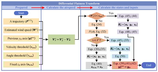
Figure 3. The differential flatness transform process of a tail-sitter flying-wing UAV.

Remark 4. 

Given that the derived differential flatness transform functions and singularity conditions stem from ${\mathit{V}}_a^I$, they can naturally integrate ${\mathit{W}}^I$ into ${\mathit{V}}_g^I$.

5. Control Architecture

In this section, we introduce the trajectory tracking control architecture (see Figure 4) tailored for aggressive flights, leveraging the previous discussion of the tail-sitter flying-wing UAV’s differential flatness alongside wind estimation. Firstly, a third-order smooth flat-output trajectory is meticulously planned offline utilizing a trajectory generation method [26]. This method leverages optimization technology to formulate the trajectory planning problem, aiming to identify a smooth and dynamically feasible trajectory with minimal flight time, control effort, and adherence to a sequence of waypoints. Subsequently, the differential flatness transform, as detailed in Section 4.3, facilitates the mapping of the flat output trajectory to the desired state trajectory ${\left({\mathit{X}}_{full}\right)}_{\mathrm{d}}$ and desired control input trajectory ${\left({\mathit{U}}_{full}\right)}_{\mathrm{d}}$. This transformation accommodates the estimated environmental wind introduced in Section 3, while also addressing the singularity conditions articulated in Section 4.2. The calculated desired state trajectories ${\left({\mathit{X}}_{full}\right)}_{\mathrm{d}}$ are tracked by a unified global controller [8], which computes the control commands ${\left({\mathit{U}}_{full}\right)}_{\mathrm{c}}$. Finally, the obtained ${\left({\mathit{U}}_{full}\right)}_{\mathrm{d}}$ is amalgamated with ${\left({\mathit{U}}_{full}\right)}_{\mathrm{c}}$ in the form of a feedforward control term, yielding the final control inputs ${\left({\mathit{U}}_{full}\right)}_{\mathrm{f}}$. In our controller deployment process, we directly map the thrust acceleration commands in ${\left({\mathit{U}}_{full}\right)}_{\mathrm{f}}$ to the collective throttle settings of two motors using the mixer described in [8].

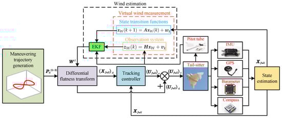
Figure 4. Control architecture.

6. Real-World Flight Tests

In this section, the performance of the controller is evaluated on various agile trajectories featuring high speed and large accelerations. These trajectories are considered highly challenging even by expert human pilots:

• Climbing turn (Figure 5a): the UAV rapidly changes its heading angle from $0°$ to $270°$ during the climb. During the turn, the reference trajectory reaches a peak yaw angular rate of 339 deg/s and a peak acceleration of 2.6 g.
  

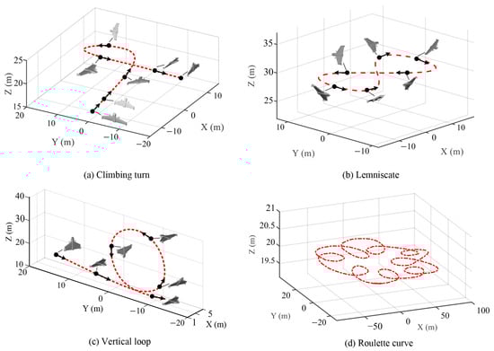  Figure 5. Illustration of the target agile trajectories.
• Lemniscate (Figure 5b): this trajectory resembles the shape of the numeral “8” when viewed from above. The maneuver involves a series of coordinated turns and rolls, creating two intersecting loops in the sky. This reference trajectory has a constant target speed of 6 $\mathrm{m}/\mathrm{s}$ and reaches a peak yaw angular rate of 135 deg/s and a peak acceleration of 1.7 g.
• Vertical loop (Figure 5c): In this maneuver, the UAV pitches up sharply, entering a vertical climb until it reaches its maximum altitude. At the apex of the climb, the UAV inverts, with its nose pointed downward, continuing the rotation until it completes a full circle. Throughout the maneuver, the UAV’s pitch attitude changes continuously, starting from a vertical climb, passing through an inverted flight at the top of the loop, and returning to level flight upon completion of the rotation. This trajectory has a constant target speed of 15 $\mathrm{m}/\mathrm{s}$ and a peak acceleration of 2.04 g.
• Roulette curve trajectory (Figure 5d): the trajectory consists of several fast successive turns. It is defined as

  $$\left[\begin{array}{c}x\left(t\right)\\ y\left(t\right)\\ z\left(t\right)\end{array}\right]=\left[\begin{array}{c}{r}_{1}cos{k}_{1}t+r_{2}cos{k}_{2}t+r_{3}sin{k}_{3}t\\ r_{4}sin{k}_{1}t+r_{5}sin{k}_{2}t+r_{6}cos{k}_{3}t\\ r_z\end{array}\right],$$

  (58)

  where $r_1=52$, $r_2=18$, $r_3=9$, $r_4=12$, $r_5=6$, $r_6=5$, $k_1=0.56$, $k_2=1.4$, $k_3=1.2$, and $r_z=20$.

Please note that all trajectory tracking tests are conducted within the context of a standard tail-sitter flying-wing UAV operation. Initially, the vehicle assumes a hovering position at the starting point before commencing trajectory tracking. Subsequently, it smoothly transitions into the cruise phase to facilitate accurate trajectory tracking.

As outlined in Section 1, the agile maneuver flight control problem for tail-sitter flying-wing UAVs has received limited attention in existing literature. This study builds upon and extends the findings presented in [8], refining the methodologies proposed therein. Therefore, for comparative purposes, we exclusively adopt the control methodology described in [8] as a benchmark in our investigation.

6.1. Experimental Setup

The fight tests are conducted in an outdoor flight space (see Figure 6b) with a wind speed range of [1.3, 4.7] m/s. The used tail-sitter flying-wing UAV is shown in Figure 6a. It is a front-pull flying-wing UAV with a wingspan of 0.98 m primarily composed of extruded polystyrene foam and fiberglass, bonded together with epoxy resin to form the entire frame. This vehicle is equipped with two Gemfan Hulkie 5055 propellers and T-Motor F40 motors. The control surfaces are managed using MKS85i micro servos, while a uniaxial pitot tube is mounted on the nose of the airframe.

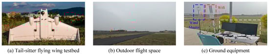
Figure 6. Flight environment and equipment.

The flight control unit consists of a Pixhawk V5 autopilot and an onboard computer (NVIDIA Jetson Nano). Notably, the presented control algorithms are implemented on the onboard computer, with the autopilot solely responsible for processing sensor data and transmitting control input signals to the actuators. Communication between the onboard computer and the autopilot is established using MAVROS. Position measurements, provided by a GPS module, are transmitted to the vehicle at a rate of 20 Hz. Figure 6c illustrates the ground equipment utilized, comprising a ground control station (GCS), a Wi-Fi router, and a Wind Master 3D sonic anemometer. The GCS is employed to monitor real-time flight status information and transmit control instructions. The Wi-Fi router establishes a local area network facilitating the connection between the GCS and the autopilot.

It is important to highlight that the extended Kalman filter (EKF) and differential flatness transformations used in our approach may present challenges for resource-constrained UAVs, especially during real-time operations. In our flight tests, we employed the Pixhawk V5 autopilot and the onboard NVIDIA Jetson Nano computer, both of which offer sufficient computational power and speed for the proposed method. However, to improve the feasibility of our approach on hardware platforms with more limited computational resources, we propose the following four recommendations: (1) Simplifying the EKF or using a lightweight variant such as the unscented Kalman filter (UKF) or particle filter could reduce the computational burden while maintaining acceptable estimation accuracy. (2) Reducing the complexity of the system models used in the differential flatness transformations could decrease the computational demands, making the algorithms more suitable for lower-power hardware. (3) Implementing more computationally efficient numerical methods, such as faster matrix inversion techniques or using approximate methods for linearization, can help reduce the real-time computational demands. (4) Reducing the frequency of sensor updates or implementing adaptive sampling techniques may help to lower the computational load during real-time operations.

6.2. Algorithm Deployment

The wind estimation algorithm, flatness transform, and global tracking controller are all implemented on the onboard computer and communicate via the robot operating system (ROS). The wind estimation algorithm is executed in ROS sub-node program 1, called Wind_Estimation.cpp, which sends the wind estimation results (${\mathit{W}}^I$) to a custom topic, Wind_Estimation_Result, in real time. The time step for the wind estimation algorithm is determined by the update rate of the developed state estimator.

The flatness transform algorithm is handled in ROS sub-node program 2, Flatness_Transform.cpp, which receives the wind estimation results (${\mathit{W}}^I$) from the W_Est_Res topic and calculates the desired state trajectory ${\left({\mathit{X}}_{full}\right)}_{\mathrm{d}}$ and desired control input trajectory ${\left({\mathit{U}}_{full}\right)}_{\mathrm{d}}$. These values are transmitted to the custom topics State_Traj and Control_Traj, respectively. The flatness transform incorporates the aerodynamic model of the tail-sitter flying wing, which was identified through wind tunnel tests conducted in previous work [22]. A database containing aerodynamic coefficients for all operating conditions has been formed. To refine the model, a series of normal and inverted level flight tests are conducted at various speeds and angles of attack. Flight data, including motor PWM, vehicle velocity, and attitude, are collected. The rotor speed is calculated from the motor PWM, and the incoming airflow is a combination of the estimated wind speed and the vehicle’s inertial speed. The total thrust is then computed using the open-source APC propeller model. By excluding the propeller thrust, the lift and drag forces acting on the vehicle are determined, leading to the values of lift and drag coefficients ($C_L$ and $C_D$) at different angles of attack ($\alpha$). The aerodynamic model is iteratively refined through flight tests conducted across a range of speeds to ensure stable flight performance.

The tracking control algorithm is executed in ROS sub-node program 3, Agile_Control.cpp. This program receives the desired state and control input trajectories ${\left({\mathit{X}}_{full}\right)}_{\mathrm{d}}$ and ${\left({\mathit{U}}_{full}\right)}_{\mathrm{d}}$ from the State_Traj and Control_Traj topics and transmits the calculated control inputs to the autopilot. The vehicle then follows the desired high-maneuverability trajectory as determined by the control signals.

6.3. Climbing Turn Trajectory

The performance comparison between the two control methods for tracking climbing turn trajectories is depicted in Figure 7 and summarized in Table 1. Both the method [8] and our approach effectively stabilize the climbing turn flight condition. However, our method exhibits superior tracking performance in terms of both root mean square (RMS) tracking error and maximum tracking error. Notably, Table 1 highlights a substantial improvement, with a 21.2% reduction in RMS position tracking error and a 21.4% decrease in maximum acceleration tracking error. Throughout the entire trajectory, our controller achieves precise tracking of the position reference within an RMS error of 52 cm, the velocity reference within 2.44 m/s RMS, and the acceleration reference within 4.86 $\mathrm{m}/{\mathrm{s}}^2$ RMS.

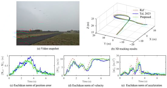
Figure 7. Experimental results for climbing turn trajectory. The blue line denotes the method in [8].

Table 1. Performance data of the two methods for tracking climbing turn trajectory (SD is the abbreviation for standard deviation).

Index	Method [8]	Proposed	Improvement
RMS ${∥{\mathbf{X}}_{\mathrm{ref}}-\mathbf{X}∥}_2$	0.66 m	0.52 m	21.2%
max ${∥{\mathbf{X}}_{\mathrm{ref}}-\mathbf{X}∥}_2$	0.94 m	0.80 m	14.9%
SD ${∥{\mathbf{X}}_{\mathrm{ref}}-\mathbf{X}∥}_2$	0.53 m	0.47 m	11.3%
RMS ${∥{\mathbf{V}}_{\mathrm{ref}}-\mathbf{V}∥}_2$	2.91 m/s	2.44 m/s	17.2%
max ${∥{\mathbf{V}}_{\mathrm{ref}}-\mathbf{V}∥}_2$	4.12 m/s	3.79 m/s	9.7%
SD ${∥{\mathbf{V}}_{\mathrm{ref}}-\mathbf{V}∥}_2$	1.29 m/s	1.11 m/s	11.9%
RMS ${∥{\mathbf{a}}_{\mathrm{ref}}-\mathbf{a}∥}_2$	5.77 $\mathrm{m}/{\mathrm{s}}^2$	4.86 $\mathrm{m}/{\mathrm{s}}^2$	15.6%
max ${∥{\mathbf{a}}_{\mathrm{ref}}-\mathbf{a}∥}_2$	10.25 $\mathrm{m}/{\mathrm{s}}^2$	8.01 $\mathrm{m}/{\mathrm{s}}^2$	21.4%
SD ${∥{\mathbf{a}}_{\mathrm{ref}}-\mathbf{a}∥}_2$	4.85 $\mathrm{m}/{\mathrm{s}}^2$	4.02 $\mathrm{m}/{\mathrm{s}}^2$	16.5%

During the turn, our method enables the vehicle to execute a roll angle close to $90°$ with a peak acceleration of 2.1 g. The attitude responses of our method throughout the flight are illustrated in Figure 8. It is observed that, during the turn, peak yaw and roll rates reach 319 deg/s and 461 deg/s, respectively. Additionally, brief saturation of the actuators occurs, leading to a temporary loss of position tracking accuracy. However, once the saturation issue is resolved, the vehicle promptly reduces the position tracking error to below 0.3 m before exiting the turn.

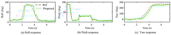
Figure 8. Attitude responses of the proposed method for climbing turn trajectory.

6.4. Lemniscate Trajectory

The experimental results presented in Figure 9 demonstrate the tracking performance of our tail-sitter flying-wing UAV as it follows a Lemniscate trajectory, maintaining a constant flight speed of 6 m/s. This trajectory entails rapid and smooth consecutive turns while ensuring stable roll and yaw, along with effective maneuverability. Throughout the trajectory, the UAV maintains a target yaw angle perpendicular to its velocity, enabling coordinated flight. A comparison between the reference and flown trajectories for one lap is illustrated in Figure 9, highlighting significant disparities in tracking performance between method [8] and our approach.

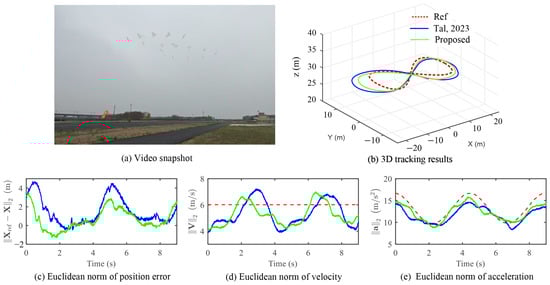
Figure 9. Experimental results for Lemniscate trajectory. The blue line denotes the method in [8].

Quantitative analysis, as shown in Table 2, reveals that our control method attains a maximum position tracking error of 3.49 m, with a RMS error of 5.8 m, a maximum velocity tracking error of 1.97 m/s, with a RMS error of 3.25 m/s, and a maximum acceleration tracking error of 2.81 $\mathrm{m}/{\mathrm{s}}^2$, with a RMS error of 3.59 $\mathrm{m}/{\mathrm{s}}^2$. In comparison with method [8], our method yields improvements of 22.6%, 17.9%, and 18.7% in RMS position, velocity, and acceleration tracking errors, respectively. Notably, from Figure 9b,c, it is evident that the most significant position deviation of our controller happens on the outermost side of the Lemniscate trajectory, in which the tail-sitter flying-wing UAV fails to track the desired acceleration. However, during the middle section, the vehicle accelerates to compensate for this deviation, thereby reducing the position error.

Table 2. Performance data of the two methods for tracking Lemniscate trajectory (SD is the abbreviation for standard deviation).

Index	Method [8]	Proposed	Improvement
RMS ${∥{\mathbf{X}}_{\mathrm{ref}}-\mathbf{X}∥}_2$	7.52 m	5.80 m	22.6%
max ${∥{\mathbf{X}}_{\mathrm{ref}}-\mathbf{X}∥}_2$	4.63 m	3.49 m	26.1%
SD ${∥{\mathbf{X}}_{\mathrm{ref}}-\mathbf{X}∥}_2$	2.60 m	2.29 m	11.5%
RMS ${∥{\mathbf{V}}_{\mathrm{ref}}-\mathbf{V}∥}_2$	3.99 m/s	3.25 m/s	17.9%
max ${∥{\mathbf{V}}_{\mathrm{ref}}-\mathbf{V}∥}_2$	2.08 m/s	1.97 m/s	5.0%
SD ${∥{\mathbf{V}}_{\mathrm{ref}}-\mathbf{V}∥}_2$	1.17 m/s	1.01 m/s	13.6%
RMS ${∥{\mathbf{a}}_{\mathrm{ref}}-\mathbf{a}∥}_2$	4.31 $\mathrm{m}/{\mathrm{s}}^2$	3.59 $\mathrm{m}/{\mathrm{s}}^2$	18.7%
max ${∥{\mathbf{a}}_{\mathrm{ref}}-\mathbf{a}∥}_2$	3.08 $\mathrm{m}/{\mathrm{s}}^2$	2.81 $\mathrm{m}/{\mathrm{s}}^2$	6.7%
SD ${∥{\mathbf{a}}_{\mathrm{ref}}-\mathbf{a}∥}_2$	1.48 $\mathrm{m}/{\mathrm{s}}^2$	1.20 $\mathrm{m}/{\mathrm{s}}^2$	18.9%

Figure 10 displays the desired and actual attitude. The maximum attitude tracking error peaks briefly during the turn, with the tail-sitter flying-wing UAV experiencing a pitch error of 7 degrees. Accurate pitch attitude control for these vehicles during agile flight is inherently difficult, given the absence of dedicated elevators for pitch adjustment, which likely results in noticeable position tracking errors during turning maneuvers. In this trajectory, the roll angle nearly reaches 1 rad, which correlates with the acceleration reaching close to 1.8 g in Figure 9e. Overall, our employed attitude controller effectively tracks the dynamic attitude command, maintaining an attitude error of less than 7 degrees on the $x_B$ and $y_B$ axes and less than 19 degrees on the $z_B$ axis throughout the remainder of the trajectory.

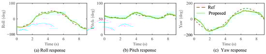
Figure 10. Attitude responses of the proposed method for Lemniscate trajectory.

6.5. Vertical Loop Trajectory

The flight results for the vertical loop trajectory are depicted in Figure 11 and Figure 12. Both the vehicles utilizing method [8] and our approach successfully complete this loop trajectory with a radius of approximately 9 m in 4.7 s. It is noteworthy that the target flight speed is set relatively high at 15 m/s to ensure the vehicle can execute a loop with a full upward pitch rotation. Through multiple experiments, we have observed distinct behaviors based on the flight speed. When flown at slow speeds (below 3.7 m/s), the loop trajectory is feasible, with the vehicle adopting a hover attitude with $\theta \approx \pi /2$ rad. Conversely, at higher speeds (above 7.5 m/s), the vehicle executes a loop with a full upward pitch rotation. Intermediate speeds (around 5 m/s) prove impractical for performing a loop, necessitating the vehicle to rapidly pitch back down at the apex of the circular segment due to flap deflection limits.

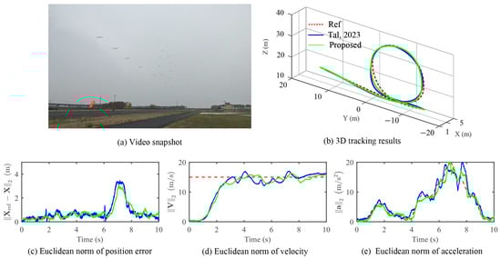
Figure 11. Experimental results for vertical loop trajectory. The blue line denotes the method in [8].

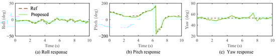
Figure 12. Attitude responses of the proposed method for the vertical loop trajectory.

From the data presented in Table 3, our control method attains a maximum position tracking error of 2.51 m, with a RMS error of 3.98 m. The maximum velocity tracking error stands at 2.87 m/s, with a RMS error of 3.11 m/s, and the maximum acceleration tracking error reaches 4.10 $\mathrm{m}/{\mathrm{s}}^2$, with a RMS error of 4.01 $\mathrm{m}/{\mathrm{s}}^2$. Comparatively, our method showcases improvements of 12.9%, 11.4%, and 12.1% in RMS position, velocity, and acceleration tracking errors, respectively, when contrasted with method [8]. It is notable that both controllers exhibit the largest position deviation when the vehicle exits the final circular segment. This phenomenon can be attributed to the vehicle encountering the highest acceleration change in the closing stages of the vertical loop trajectory. Due to the UAV’s inertia, the position response lags behind the acceleration change, consequently leading to substantial position tracking errors.

Table 3. Performance data of the two methods for tracking vertical loop trajectory (SD is the abbreviation for standard deviation).

Index	Method [8]	Proposed	Improvement
RMS ${∥{\mathbf{X}}_{\mathrm{ref}}-\mathbf{X}∥}_2$	4.57 m	3.98 m	12.9%
max ${∥{\mathbf{X}}_{\mathrm{ref}}-\mathbf{X}∥}_2$	2.79 m	2.51 m	10.0%
SD ${∥{\mathbf{X}}_{\mathrm{ref}}-\mathbf{X}∥}_2$	1.07 m	0.99 m	7.4%
RMS ${∥{\mathbf{V}}_{\mathrm{ref}}-\mathbf{V}∥}_2$	3.52 m/s	3.11 m/s	11.4%
max ${∥{\mathbf{V}}_{\mathrm{ref}}-\mathbf{V}∥}_2$	3.15 m/s	2.87 m/s	9.6%
SD ${∥{\mathbf{V}}_{\mathrm{ref}}-\mathbf{V}∥}_2$	1.92 m/s	1.76 m/s	8.3%
RMS ${∥{\mathbf{a}}_{\mathrm{ref}}-\mathbf{a}∥}_2$	4.56 $\mathrm{m}/{\mathrm{s}}^2$	4.01 $\mathrm{m}/{\mathrm{s}}^2$	12.1%
max ${∥{\mathbf{a}}_{\mathrm{ref}}-\mathbf{a}∥}_2$	5.77 $\mathrm{m}/{\mathrm{s}}^2$	4.10 $\mathrm{m}/{\mathrm{s}}^2$	28.0%
SD ${∥{\mathbf{a}}_{\mathrm{ref}}-\mathbf{a}∥}_2$	3.17 $\mathrm{m}/{\mathrm{s}}^2$	2.96 $\mathrm{m}/{\mathrm{s}}^2$	6.6%

6.6. Roulette Curve Trajectory

As a final demonstration of the feasibility of our designed control method, we conduct a challenging agile maneuver flight test in which the UAV is commanded to track a roulette curve trajectory. This trajectory entailed rapid and successive turns, necessitating precise tracking due to the swift changes in acceleration, demanding high angular rates and accelerations. The tracking results, depicted in Figure 13, along with performance metrics outlined in Table 4, reaffirm the efficacy of our approach compared to the method proposed in [8]. Specifically, our controller achieved a position tracking error of 1.12 m RMS, with a maximum error of 0.88 m. Additionally, it demonstrated a velocity tracking error of 3.71 m/s RMS, with a maximum error of 5.99 m/s, and an acceleration tracking error of 6.51 $\mathrm{m}/{\mathrm{s}}^2$ RMS, with a maximum error of 4.29 $\mathrm{m}/{\mathrm{s}}^2$. Notably, our method outperformed the approach in [8], showcasing improvements of 15.3%, 9.2%, and 14.4% in RMS position, velocity, and acceleration tracking errors, respectively.

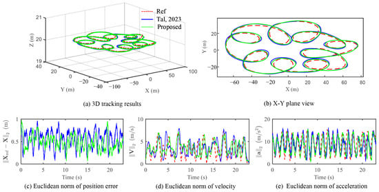
Figure 13. Experimental results for roulette curve trajectory. The blue line denotes the method in [8].

Table 4. Performance data of the two methods for tracking roulette curve trajectory (SD is the abbreviation for standard deviation).

Index	Method [8]	Proposed	Improvement
RMS ${∥{\mathbf{X}}_{\mathrm{ref}}-\mathbf{X}∥}_2$	1.31 m	1.12 m	15.3%
max ${∥{\mathbf{X}}_{\mathrm{ref}}-\mathbf{X}∥}_2$	0.91 m	0.88 m	3.2%
SD ${∥{\mathbf{X}}_{\mathrm{ref}}-\mathbf{X}∥}_2$	0.56 m	0.49 m	12.5%
RMS ${∥{\mathbf{V}}_{\mathrm{ref}}-\mathbf{V}∥}_2$	4.09 m/s	3.71 m/s	9.2%
max ${∥{\mathbf{V}}_{\mathrm{ref}}-\mathbf{V}∥}_2$	6.21 m/s	5.99 m/s	3.5%
SD ${∥{\mathbf{V}}_{\mathrm{ref}}-\mathbf{V}∥}_2$	3.42 m/s	3.01 m/s	11.9%
RMS ${∥{\mathbf{a}}_{\mathrm{ref}}-\mathbf{a}∥}_2$	7.64 $\mathrm{m}/{\mathrm{s}}^2$	6.51 $\mathrm{m}/{\mathrm{s}}^2$	14.4%
max ${∥{\mathbf{a}}_{\mathrm{ref}}-\mathbf{a}∥}_2$	4.58 $\mathrm{m}/{\mathrm{s}}^2$	4.29 $\mathrm{m}/{\mathrm{s}}^2$	6.3%
SD ${∥{\mathbf{a}}_{\mathrm{ref}}-\mathbf{a}∥}_2$	2.66 $\mathrm{m}/{\mathrm{s}}^2$	2.25 $\mathrm{m}/{\mathrm{s}}^2$	15.0%

6.7. Wind Estimation Results

To evaluate the effectiveness of the proposed wind estimation algorithm, we utilize data obtained from both a static hover test and the tracking of the roulette curve trajectory. The static hover test evaluates our method’s performance during the hover stage, while data from the roulette curve flight allow us to assess its performance during the transition and cruising phases. As illustrated in Figure 6b, a 3D sonic anemometer (Wind Master) is positioned 2.0 m above the ground to measure the actual ground wind data. This instrument provided precise wind status information, including speed and direction. Further details regarding the anemometer can be found in Figure 14. To obtain wind speed measurements at the altitude of the vehicle, we employ the wind profile power law [27]:

$$∥{\mathit{W}}_h^I∥=∥{\mathit{W}}_{\mathrm{ref}}^I∥{\left({\displaystyle \frac{h}{h_{\mathrm{ref}}}}\right)}^p,$$

(59)

where h is the vehicle’s altitude; $h_{ref}=2 \mathrm{m}$ is the installation height of the anemometer; $∥{\mathit{W}}_{\mathrm{ref}}^I∥$ is the wind speed at height $h_{ref}$; $∥{\mathit{W}}_{\mathrm{h}}^I∥$ is the magnitude of the wind at height h; $p=0.25$ is the power-law exponent. This law has been widely utilized for estimating the atmospheric wind speed profile.

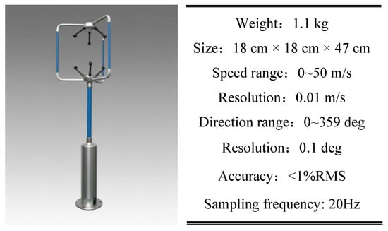
Figure 14. Three-dimensional (3D) Wind Master anemometer.

The effectiveness of our wind estimation method is demonstrated in Figure 15, where it is compared with ground measurements obtained during the hover test. Figure 15c,d depict the estimated wind speed and direction, respectively, along with $3\sigma$ bounds, plotted on a timescale for clarity. Notably, Figure 15d shows the wind direction within the range of $\left[-180°,180°\right]$ for easy comparison, with $0°$ denoting a northward wind direction. The ground-truth wind direction is observed to be $10°$. Table 5 presents the statistical measurements of wind estimation error, including maximum absolute error, maximum relative error, root mean squared error (RMS), and error margins. Overall, the proposed wind estimation algorithm demonstrates an accurate estimation of the wind direction, closely aligning with the actual direction. Additionally, the estimated wind speed fluctuates around 2.5 m/s, mirroring the ground measurements closely. These findings underscore the effectiveness of our presented wind estimation method, particularly in the context of hover flight for a tail-sitter flying-wing UAV.

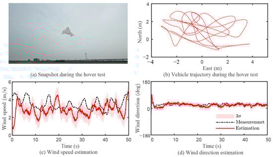
Figure 15. Wind estimation results during the hover tests.

Table 5. Statistical measurement of wind estimation error during the hover tests.

Error	Maximum Absolute Error	Maximum Relative Error	Root Mean Squared Error	Error Margin	Standard Deviation
Wind speed	2.62 m/s	0.97 m/s	1.86 m/s	1.13 m/s	1.17 m/s
Wind direction	19.8 deg	2.15 deg	11.77 deg	12.93 deg	11.56 deg

Figure 16 illustrates the wind estimation results obtained during the tracking of the roulette curve trajectory. Figure 16a,c showcase the estimation outcomes for both wind speed and direction, accompanied by $3\sigma$ bounds, while Figure 16b,d display the corresponding estimation errors. The wind estimator is initialized with a wind speed of approximately 0 m/s and a wind direction of about $0°$. Throughout the test, the working frequency of EKF is 10 Hz. Table 6 presents the statistical measurements of wind estimation error during the tracking of the roulette curve trajectory. From the results, it can be known that the proposed estimation method performs admirably in both direction and speed estimation. The root mean square errors for wind direction and speed are calculated to be $37.91°$ and 1.94 m/s. Additionally, Figure 16 includes a comparison of directions and speeds obtained from estimators utilizing only virtual measurements versus those fused with a pitot tube. Table 7 presents the statistical measurements of wind estimation error during the tracking of the roulette curve trajectory using the proposed wind estimation method (no pitot). It is notable that for most of the cruise phase, the performance of the estimator relying solely on virtual measurements deteriorates compared to the one fused with both virtual measurements and a pitot tube. However, during the forward transition (FT) and backward transition (BT) phases, the disparity in estimation between the two methods is minimal.

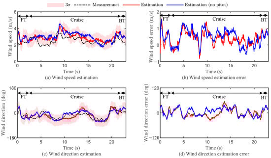
Figure 16. Wind estimation results during the tracking of the roulette curve trajectory.

Table 6. Statistical measurement of wind estimation error during the tracking of the roulette curve trajectory using the proposed wind estimation method.

Error	Maximum Absolute Error	Maximum Relative Error	Root Mean Squared Error	Error Margin	Standard Deviations
Wind speed	1.66 m/s	0.59 m/s	1.94 m/s	1.37 m/s	0.87 m/s
Wind direction	59.50 deg	1.64 deg	37.91 deg	38.52 deg	24.25 deg

Table 7. Statistical measurement of wind estimation error during the tracking of the roulette curve trajectory using the proposed wind estimation method (no pitot).

Error	Maximum Absolute Error	Maximum Relative Error	Root Mean Squared ERROR	Error Margin	Standard Deviations
Wind speed	1.69 m/s	0.62 m/s	1.98 m/s	1.49 m/s	0.68 m/s
Wind direction	42.64 deg	1.59 deg	43.01 deg	46.77 deg	24.16 deg

7. Conclusions

This study presents a novel control architecture for a tail-sitter flying-wing UAV, aiming to achieve more robust and accurate tracking control of agile trajectories. Central to this architecture is the derived differential flatness transform, facilitating the mapping of desired maneuver trajectories to state-input trajectories. Unlike conventional approaches relying on simplified models, our methodology derives complete differential flatness transform functions from a comprehensive aerodynamics model that incorporates wind effects, addressing and resolving singularity conditions comprehensively. For accurate wind estimation without resorting to costly and complex instruments, we propose a novel wind estimation method leveraging low-cost sensors, including an IMU sensor, a pitot tube, and a GPS unit. This method, grounded in the principles of “wind triangle”, also exploits aerodynamic relationships to enhance estimation accuracy. The resultant state-input trajectory is tracked using an existing controller from the reference literature.

Validation of the control system is conducted through extensive real-world flights with a tail-sitter flying-wing UAV prototype. Notably, we demonstrate multiple agile flights in windy outdoor environments, a rarity in prior literature. Results underscore the improved robustness of our control design against external disturbances compared to existing methods. Furthermore, validation of the wind estimation method reveals agreement between estimated and ground-measured wind magnitude and direction, with approximate MSE errors of less than 0.58 m/s in wind speed and less than $15.09°$ in wind direction.

While our current control method showcases promising performance, several limitations warrant consideration to enhance its suitability for widespread deployment. Firstly, our method relies entirely on the state estimation and signal processing algorithms provided by PX4. However, using pre-existing algorithms may have certain limitations. Firstly, this approach has limited adaptability to other flight control systems. When using new hardware platforms, PX4’s state estimation and signal processing algorithms may no longer be applicable. Furthermore, this research highly depends on sensor data from the aircraft, and since the algorithms in PX4 are relatively simple, they may not be capable of handling more demanding signal processing needs in harsh environments. Some feasible solutions for measurement noise and sensor uncertainties include: (1) Implementing robust filtering techniques, such as Particle Filters, to better account for noise and sensor inaccuracies. (2) Integrating fault detection and isolation (FDI) systems to identify and manage sensor failures. (3) Utilizing sensor fusion algorithms to combine data from multiple sensors, thus improving the accuracy and robustness of the system. (4) Exploring adaptive signal processing methods that adjust to changing environmental conditions and sensor performance over time. We will continue to explore and improve upon this area in future work. Secondly, in our controller deployment process, we directly map the thrust acceleration commands to the collective throttle settings of two motors. This approach ignores the impact of the motor’s internal dynamics and propeller inflow, leading to notable discrepancies between commanded and measured thrust acceleration. Implementing a simple controller that utilizes real-time acceleration measurements to track thrust acceleration commands could mitigate this issue. Thirdly, the proposed method for estimating wind speed exclusively targets uniform wind fields. redThis assumption of uniform wind conditions limits the method’s adaptability in more complex environments with variable wind fields, such as high-altitude settings and urban canyons. To address this, we plan to integrate more advanced atmospheric models and real-time multi-sensor fusion techniques in the future, aiming to improve the method’s applicability in challenging environments. Fourthly, the proposed approach relies on a specific set of sensors (IMU, pitot tube, GPS), which, although cost-effective compared to the high-precision sensors used in larger aircraft, are more susceptible to failures during flight. Therefore, developing a wind estimation algorithm capable of tolerating sensor failures is not only essential but also critical for enhancing both flight safety and system robustness. Lastly, this study focuses on a specific UAV design (tail-sitter flying wing) and corresponding trajectory patterns, which limits the general applicability of our findings to other UAV types or mission profiles. This focus is due to the reliance of the proposed method on the dynamic model of the tail-sitter flying wing, making it particularly suitable for this configuration. In the future, we plan to develop a more generalized high-maneuverability control method that does not depend on a specific model. We also intend to test this method on various UAV types to demonstrate its broader applicability.

References

- Wagter, C.D.; Remes, B.; Smeur, E.; van Tienen, F.; Ruijsink, R.; Hecke, K.; der Horst, E. The NederDrone: A hybrid lift, hybrid energy hydrogen UAV. Int. J. Hydrogen Energy 2021, 46, 16003–16018. [Google Scholar] [CrossRef]
- Gu, H.; Lyu, X.; Li, Z.; Shen, S.; Zhang, F. Development and Experimental Verification of a Hybrid Vertical Take-Off and Landing (VTOL) Unmanned Aerial Vehicle(UAV). In Proceedings of the 2017 International Conference on Unmanned Aircraft Systems (ICUAS), Miami, FL, USA, 13–16 June 2017; pp. 160–169. [Google Scholar]
- He, C.; Chen, G.; Sen, X.; Li, S.; Li, Y. Geometrically compatible integrated design method for conformal rotor and nacelle of distributed propulsion tilt-wing UAV. Chin. J. Aeronaut. 2023, 36, 229–245. [Google Scholar] [CrossRef]
- Bauersfeld, L.; Spannagl, L.; Ducard, G.J.J.; Onder, C.H. MPC Flight Control for a Tilt-Rotor VTOL Aircraft. IEEE Trans. Aerosp. Electron. Syst. 2021, 57, 2395–2409. [Google Scholar] [CrossRef]
- Li, Y.; Dong, H.; Li, H.; Zhang, X.; Zhang, B.; Xiao, Z. Multi-block SSD based on small object detection for UAV railway scene surveillance. Chin. J. Aeronauts 2020, 33, 1747–1755. [Google Scholar] [CrossRef]
- Alzahrani, B.; Oubbati, O.S.; Barnawi, A.; Atiquzzaman, M.; Alghazzawi, D. UAV assistance paradigm: State-of-the-art in applications and challenges. J. Netw. Comput. Appl. 2020, 166, 102706. [Google Scholar] [CrossRef]
- Woellner, R.; Wagner, T.C. Saving species, time and money: Application of unmanned aerial vehicles (UAVs) for monitoring of an endangered alpine river specialist in a small nature reserve. Biol. Conserv. 2019, 233, 162–175. [Google Scholar] [CrossRef]
- Tal, E.; Karaman, S. Global Incremental Flight Control for Agile Maneuvering of a Tailsitter Flying Wing. J. Guid. Control. Dyn. 2023, 45, 2332–2349. [Google Scholar] [CrossRef]
- Tal, E.; Ryou, G.; Karaman, S. Aerobatic Trajectory Generation for a VTOL Fixed-Wing Aircraft Using Differential Flatness. IEEE Trans. Robot. 2023, 39, 4805–4819. [Google Scholar] [CrossRef]
- Lustosa, L.R.; Defay, F.; Moschetta, J.M. Global singularity-free aerodynamic model for algorithmic flight control of tail sitters. J. Guid. Control. Dyn. 2019, 42, 303–316. [Google Scholar] [CrossRef]
- Pfeifle, O.; Fichter, W. Cascaded incremental nonlinear dynamic inversion for three-dimensional spline-tracking with wind compensation. J. Guid. Control. Dyn. 2021, 44, 1559–1571. [Google Scholar] [CrossRef]
- Yang, Y.; Zhu, J.; Zhang, X.; Wang, X. Active Disturbance Rejection Control of a Flying-Wing Tailsitter in Hover Flight. In Proceedings of the in 2018 IEEE/RSJ International Conference on Intelligent Robots and Systems (IROS), Madrid, Spain, 1–5 October 2018; pp. 6390–6396. [Google Scholar]
- Petrich, J.; Subbarao, K. On-board wind speed estimation for UAVs. In Proceedings of the AIAA Guidance, Navigation, and Control Conference, Portland, OR, USA, 8–11 August 2011. [Google Scholar]
- Langelaan, J.W.; Alley, N.; Neidhoefer, J. Wind field estimation for small unmanned aerial vehicles. J. Guid. Control. Dyn. 2011, 34, 1016–1030. [Google Scholar] [CrossRef]
- Cho, A.; Kim, J.; Lee, S.; Kee, C. Wind Estimation and Airspeed Calibration using a UAV with a Single-Antenna GPS Receiver and Pitot Tube. IEEE Trans. Aerosp. Electron. Syst. 2011, 47, 109–117. [Google Scholar] [CrossRef]
- Myschik, S.; Heller, M.; Holzapfel, F.; Sachs, G. Low-Cost Wind Measurement System For Small Aircraft. In Proceedings of the AIAA Guidance, Navigation, and Control Conference and Exhibit, Paper AIAA 2004-5240, Providence, RI, USA, 16–19 August 2004. [Google Scholar]
- Myschik, S.; Sachs, G. Flight testing an integrated wind/airdata-and navigation system for general aviation aircraft. In Proceedings of the AIAA Guidance, Navigation, and Control Conference and Exhibit, Paper AIAA 2007-6796, Hilton Head, SC, USA, 20–23 August 2007. [Google Scholar]
- Divitiis, N. Wind estimation on a lightweight vertical-takeoff-and-landing uninhabited vehicle. J. Aircr. 2003, 40, 759–767. [Google Scholar] [CrossRef]
- Demitrit, Y.; Verling, S.; Stastny, T.; Melzer, A.; Siegwart, R. Model-based wind estimation for a hovering VTOL tailsitter UAV. In Proceedings of the 2017 IEEE International Conference on Robotics and Automation (ICRA), Singapore, 29 May–3 June 2017; pp. 3945–3952. [Google Scholar]
- Lie, F.A.P.; Gebre-Egziabher, D. Synthetic air data system. J. Aircr. 2013, 50, 1234–1249. [Google Scholar] [CrossRef]
- Sun, J.; Li, B.; Wen, C.Y.; Chen, C.K. Model-Aided Wind Estimation Method for a Tail-Sitter Aircraft. IEEE Trans. Aerosp. Electron. Syst. 2020, 56, 1262–1278. [Google Scholar] [CrossRef]
- Zou, X.; Liu, Z.; Zhao, W.; Wang, L. Optimization method of transition trajectory for tail-sitter unmanned aerial vehicles. J. Beijing Univ. Aeronaut. Astronaut. 2023. [Google Scholar] [CrossRef]
- Sun, J.; Li, B.; Shen, L.; Chen, C.K.; Wen, C.Y. Dynamic modeling and hardware-in-loop simulation for a tailsitter unmanned aerial vehicle in hovering flight. In Proceedings of the in AIAA Modeling and Simulation Technologies Conference, Grapevine, TX, USA, 9–13 January 2017; pp. 9–13. [Google Scholar]
- Berman, Z.; Powell, J. The role of dead reckoning and inertial sensors in future general aviation navigation. In Proceedings of the IEEE 1998 Position Location and Navigation Symposium, Palm Springs, CA, USA, 20–23 April 1998; pp. 510–517. [Google Scholar]
- Crespillo, O.G.; Langel, S.; Joerger, M. Tight Bounds for Uncertain Time-Correlated Errors with Gauss–Markov Structure in Kalman Filtering. IEEE Trans. Aerosp. Electron. Syst. 2023, 59, 4347–4362. [Google Scholar] [CrossRef]
- Lu, G.; Cai, Y.; Chen, N.; Kong, F.; Ren, Y.; Zhang, F. Trajectory generation and tracking control for aggressive tail-sitter flights. Int. J. Robot. Res. 2024, 43, 241–280. [Google Scholar] [CrossRef]
- Molina-García, A.; Fernández-Guillamón, A.; Gómez-Lázaro, E.; Honrubia-Escribano, A.; Bueso, M.C. Vertical Wind Profile Characterization and Identification of Patterns Based on a Shape Clustering Algorithm. IEEE Access 2019, 7, 30890–30904. [Google Scholar] [CrossRef]
Disclaimer/Publisher’s Note: The statements, opinions and data contained in all publications are solely those of the individual author(s) and contributor(s) and not of MDPI and/or the editor(s). MDPI and/or the editor(s) disclaim responsibility for any injury to people or property resulting from any ideas, methods, instructions or products referred to in the content. |
© 2025 by the authors. Licensee MDPI, Basel, Switzerland. This article is an open access article distributed under the terms and conditions of the Creative Commons Attribution (CC BY) license (https://creativecommons.org/licenses/by/4.0/).