MobileRaT: A Lightweight Radio Transformer Method for Automatic Modulation Classification in Drone Communication Systems

Abstract

Nowadays, automatic modulation classification (AMC) has become a key component of next-generation drone communication systems, which are crucial for improving communication efficiency in non-cooperative environments. The contradiction between the accuracy and efficiency of current methods hinders the practical application of AMC in drone communication systems. In this paper, we propose a real-time AMC method based on the lightweight mobile radio transformer (MobileRaT). The constructed radio transformer is trained iteratively, accompanied by pruning redundant weights based on information entropy, so it can learn robust modulation knowledge from multimodal signal representations for the AMC task. To the best of our knowledge, this is the first attempt in which the pruning technique and a lightweight transformer model are integrated and applied to processing temporal signals, ensuring AMC accuracy while also improving its inference efficiency. Finally, the experimental results—by comparing MobileRaT with a series of state-of-the-art methods based on two public datasets—have verified its superiority. Two models, MobileRaT-A and MobileRaT-B, were used to process RadioML 2018.01A and RadioML 2016.10A to achieve average AMC accuracies of 65.9% and 62.3% and the highest AMC accuracies of 98.4% and 99.2% at +18 dB and +14 dB, respectively. Ablation studies were conducted to demonstrate the robustness of MobileRaT to hyper-parameters and signal representations. All the experimental results indicate the adaptability of MobileRaT to communication conditions and that MobileRaT can be deployed on the receivers of drones to achieve air-to-air and air-to-ground cognitive communication in less demanding communication scenarios.

1. Introduction

In a non-cooperative communication system, automatic modulation classification (AMC) [1] plays a crucial role in identifying the modulation scheme of communication signals to improve communication efficiency and ensure communication security. As one of the typical application scenarios of AMC, drone communication applications [2], such as remote control, telemetry, and navigation, require high-speed, low-latency, and reliable communication connectivity. AMC is able to automatically select the optimal modulation scheme based on channel conditions and the distance between drones and ground stations, thereby improving the data transmission rate and signal coverage [3]. In complex electromagnetic environments [4,5], AMC can also effectively identify and eliminate interference from other wireless devices [6], maintaining a stable and reliable connection for drone communications. As the key technique for dynamic spectrum access (DSA) [7], AMC helps to enhance spectrum utilization and communication capacity, which are particularly important for the efficient operation of drone communication systems in the crowded radio spectrum. By utilizing AMC, drone communication systems extend the battery life of drones by selecting the appropriate transmission power based on channel conditions, transmission distance, and mission requirements [8]. Moreover, AMC possesses the ability to support more communication applications and functions by seamlessly integrating them into drone communication systems, enhancing their flexibility and scalability [9]. In fact, AMC has proven to be a key contributor to drone communications by optimizing modulation schemes to improve signal quality and anti-interference capabilities, ensuring that drone communication systems can operate stably and efficiently in various environments and application scenarios.

In an actual wireless communication system, signals are not only subject to the effects of the transmitter (such as the radio frequency chain) and the receiver (such as flexible coherent receivers) [10] but also undergo changes because of a complex propagation environment with diverse types of interference [11], increasing the difficulty of modulation recognition. Specifically, channel conditions [12] cause the attenuation and distortion of signals during transmission. Multipath propagation and Doppler shifts [13] lead to a delay in spreading signals. Interference from other wireless devices and noises in the environment has a negative impact on the recognition of signal modulation methods. In addition, parameters such as signal bandwidth, sampling rate, and symbol rate all affect AMC accuracy [14]. The higher the complexity of the modulation scheme adopted, the greater the difficulty of AMC.

At present, AMC methods are mainly divided into two categories: (1) likelihood-based (LB) methods and (2) feature-based (FB) methods. The LB methods accomplish the automatic recognition of modulation schemes through Bayesian estimation, including the average likelihood ratio test (ALRT) [15], the generalized likelihood ratio test (GLRT) [16], the hybrid likelihood ratio test (HLRT) [17], and other variations. Although LB methods can adapt to various types of modulated signals, they have high computational complexity and require the accurate estimation of prior probability and likelihood function. FB methods accomplish the AMC task by constructing feature-driven machine learning classifiers. Commonly used features include cyclostationary features [18], high-order cumulants [19], and intrinsic mode functions (IMFs) [20]. The classifiers can be support vector machines (SVMs) [21], random forest (RF) [22], neural networks (NNs) [23] etc., FB methods can be easily deployed, but the design of features is labor-intensive and difficult to generalize well to different scenarios. On the other hand, machine learning models are sensitive to the performance of feature engineering. With the increasing complexity of signal waveforms and the application of high-order modulation schemes, current methods are no longer able to meet the needs of practical wireless communication systems.

In recent years, deep learning has developed impressive achievements in the field of signal processing and pattern recognition, such as spectrum sensing [24], channel modeling [25], and parameter estimation [26], and it is gradually being developed for AMC tasks. Compared with traditional classifiers [21,22,23], end-to-end deep learning models automatically learn the feature representation of input data without manual intervention or feature engineering. Driven by big data, deep learning models with large-scale parameters and nonlinear connections possess better generalization capabilities, as they can maintain stable AMC performance under different channel conditions. The most commonly used deep learning model structures can be categorized as convolutional neural network (CNN) [27,28], long short-term memory (LSTM) [29,30], graph convolutional network (GCN) [31], and transformer [32]. CNN excels in mining spatial information in signals while LSTM is more concerned with temporal information. GCN is more sensitive to the structure of data distribution. The version of transformer that introduces an attention mechanism is able to adapt to situations that contain various parameter conditions, such as different signal-to-noise ratios (SNRs). However, deep learning models require a large quantity of computing resources and power consumption, which hinders their deployment and application in drone communication systems with high real-time requirements. To be deployed in resource-constrained devices, deep learning model structures often need to be compressed and optimized, which usually leads to a decrease in AMC accuracy. Even though some lightweight neural network models (such as A-MobileNet [33] and Mobile-former [34]) and pruning methods [35] have been developed, they are not specifically designed for processing radio signals. In other words, it is difficult to directly transfer deep learning models from image classification tasks to AMC without performance loss.

1.1. Motivation

To solve the aforementioned problems, we propose a real-time AMC method based on the lightweight mobile radio transformer (MobileRaT) in this paper. The constructed radio transformer is trained iteratively, accompanied by redundant weight removal, in order to learn robust modulation knowledge from multimodal signal representations for AMC tasks. Two models of different scales deployed in workstations and edge devices are tested and compared using two public datasets, i.e., RadioML 2018.01A [36] and Radio 2016.10A [37], respectively. The experimental results, by comparing MobileRaT with a series of state-of-the-art methods, confirm its superiority. Furthermore, ablation studies are conducted to demonstrate the robustness of the proposed deep learning model to hyper-parameters and signal representations.

1.2. Novelty

The innovation of the paper is summarized as follows:

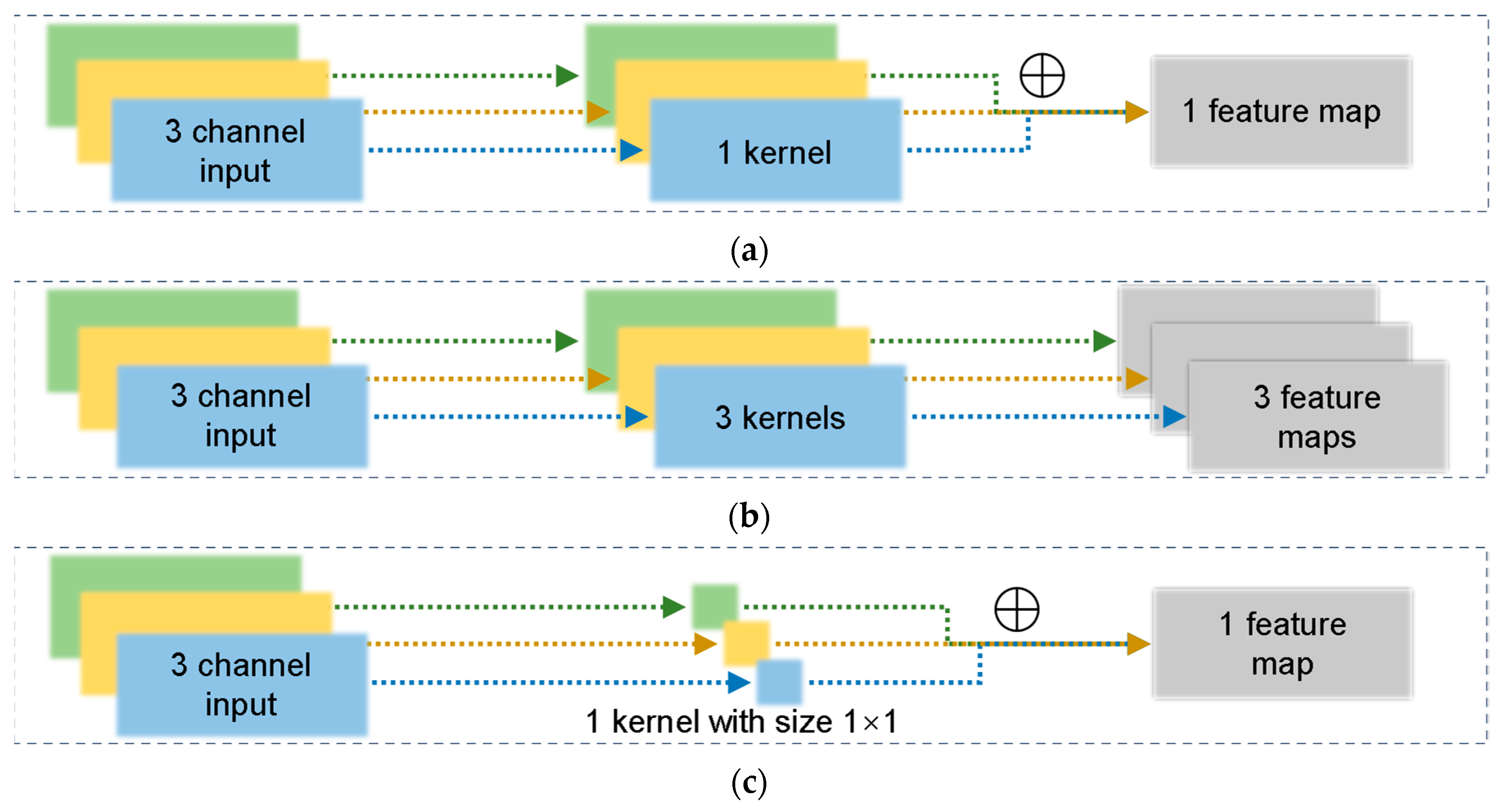
• A lightweight deep learning model combining point-wise convolution, depth-wise separable convolution, ReLU6 activation, group normalization, and other efficient computing modules was developed for AMC.
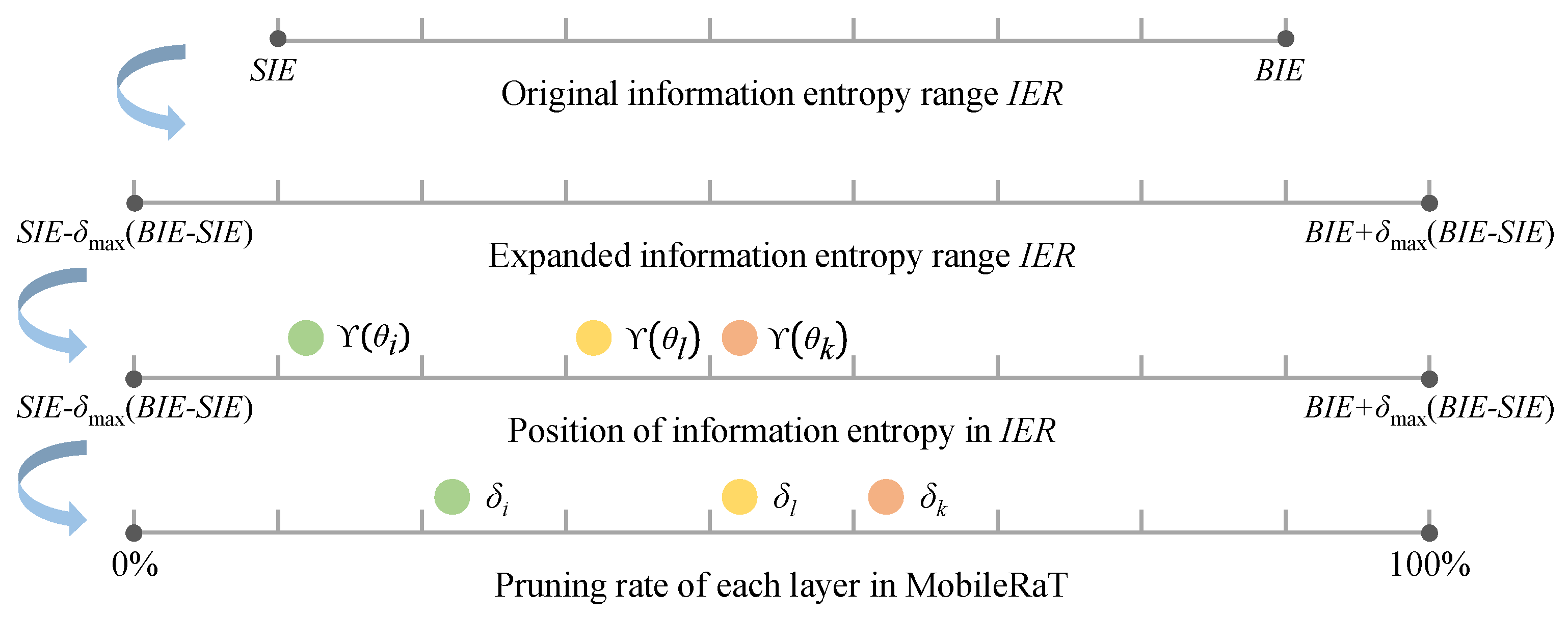
• A weight importance metric, based on information entropy, is introduced to iteratively remove redundant parameters from the model. The removal rates and training stop conditions at each epoch are carefully considered to avoid damaging the model structure.
• To the best of our knowledge, this is the first attempt in which an information-entropy-based pruning technique and a lightweight transformer are integrated and applied to processing temporal I/Q signals, ensuring AMC accuracy while improving the inference efficiency.
• Two deep learning models of different scales, MobileRaT-A and MobileRaT-B, are used to evaluate the AMC performance in realistic conditions in order to break through the limitations of storage, computing resources, and power in drone communication systems.

1.3. Organization

The rest of the paper is organized as follows. In Section 2, we describe related work on AMC. In Section 3, we introduce the proposed lightweight deep learning model, MobileRaT. The experimental results and analysis are reported in Section 4. Finally, the conclusions are summarized in Section 5.

2. Related Work

In this section, we analyze related work on AMC using both traditional LB and FB methods and modern deep learning approaches in recent years, including achievements and challenges, as well as future focus directions. The cornerstone work related to AMC is summarized in Figure 1.

Figure 1. Cornerstone work related to AMC.

2.1. LB and FB Methods

In earlier years, LB methods were widely studied to solve the AMC problem. The ALRT method [15] was designed to classify multiple phase-shift keying (MPSK) modulation schemes in additive white Gaussian noise (AWGN). Based on the GLRT assuming unknown deterministic parameters, a modulation classifier [16] was proposed to determine the number of constellation points of phase-shift keying (PSK) modulations in AWGN. In HLRT-based classifiers [17,38], energy-based detectors and likelihood-ratio-based detectors were employed to identify active subcarriers. Abu-Romoh et al. [39] proposed a moment-based maximum likelihood classifier (MbMLC) to solve the AMC problem and provided a trade-off between classification accuracy and complexity. Although these LB methods claim to have solved the AMC problem to some extent, they still face a series of challenges. In general, LB methods require high computational costs, and the computational complexity increases exponentially with the length of the sequence. Under the same computing power, it is hard for LB methods to outperform FB methods in terms of AMC performance. In addition, likelihood techniques have difficulty obtaining suitable analytical solutions for decision functions, especially in blind classification tasks where communication parameters are unknown.

FB methods improved the aforementioned issues in LB methods. Feature extraction, combined with classifier learning, usually yields local or global optimal solutions and is easy to deploy. High-order cyclic cumulants (HCCs) [18] have been widely used as features for AMC. However, the requirement of high sampling rates in communication systems greatly limits the practical application of cyclic cumulants. For the given order and time delay, a spectrum-sensing and power recognition framework based on high-order cumulants (HCs) [19] was developed, which can eliminate the adverse impact of noise power uncertainty. Carnì et al. [20] confirmed that SVMs driven by empirical mode decomposition (EMD-SVM) can identify typical analog modulation schemes, including amplitude modulation (AM), phase modulation (PM), frequency modulation (FM), and single-sideband modulation (SSB) without prior information. By combining the theories of cyclostationarity and entropy, an SVM driven by hybrid features, cyclostationarity, and information entropy (HCI-SVM) [21] was introduced to recognize digital modulation schemes. The RF-AMC method [22] utilizes different features of amplitude histograms (AHs) and swarm intelligence, and it verified its effectiveness in identifying polarization multiplexed 4/8/16/32/64 quadrature amplitude modulation (QAM). Chen et al. [40] proposed a feature extraction and mapping (FEM) algorithm for mapping radio signals to images for further classification. Compared with the original radio signal, AMC accuracy based on mapped images is slightly improved. Venkata et al. [41] constructed an ensemble-based pattern classifier for AMC, which combined decision tree (DT), discriminant analysis (DA), and K-nearest neighbor (KNN) classifiers. Shah et al. [42] combined the meta-heuristic technique with Gabor features and optimized them using the Cuckoo search algorithm (CSA) to distinguish between PSK modulations with 2–64 orders, frequency-shift keying (FSK), and QAM.

Although FB methods perform better than LB methods, there are still many factors that hinder their successful applications in practical communication scenarios, including the robustness of features, sensitivity to signal parameters, the structural complexity of classifiers, the choice of feature engineering, etc. These factors prompt researchers to shift toward end-to-end machine learning models that can more comprehensively characterize signal features, thus leading to better AMC performance.

2.2. Deep Learning Methods

At present, a large number of deep learning-based methods have been studied regarding AMC to improve adaptability and robustness to communication environments. To solve the problem of recognizing intra-class modulation schemes due to dynamic changes in wireless communication environments, Zhang et al. [3] designed a multi-scale convolutional neural network (MSNet), trained by optimizing a new loss function combining center loss and cross-entropy, to learn discriminative and separable features and improve AMC accuracy. Based on I/Q-driven outputs from different layers of the model, Chang et al. [5] proposed a hierarchical classification head-based convolutional gated deep neural network (HCGDNN) consisting of three groups of CNN, two groups of bi-directionally gated recursive units (BiGRUs), and a hierarchical classification head. Peng et al. [9] designed a deep residual neural network (DRMM) based on masked modeling to improve the AMC accuracy of deep learning with limited signal samples. Shen et al. [10] developed a multi-subsampling self-attention (MSSA) network for drone-to-ground AMC systems, for which a residual dilated module incorporating both ordinary and dilated convolutions is devised to expand the data-processing range. Then, a self-attention module is introduced to improve the AMC performance in the presence of noise interference. To solve the domain mismatch problem of deep learning structures, Zhang et al. [11] introduced a neural architecture search (NAS)-based AMC framework that automatically adjusts the connection and parameters of DNNs to find the optimal structure under a combination of training and constraints. In [13], a dual-stream spatiotemporal fusion neural network (DSSFNN)-based AMC method was developed to improve accuracy in order to assist drone communications since the DSSFNN is able to efficiently mine spatiotemporal features from modulated signals through residual blocks, LSTM blocks, and attention mechanisms. In [27], Zheng et al. proposed two-stage data augmentation (TSDA) based on spectral interference in deep learning to improve the AMC generalization ability across different communication scenarios. Wang et al. [28] developed a generalized AMC method based on multi-task learning (MTL) and considered a more realistic scenario including non-WGN and synchronization errors. To automatically recognize noisy digital modulation signals, a novel deep-LSTM model [29] was designed and successfully applied to these signals without requiring feature extraction or engineering. Zheng et al. [30] proposed an a priori regularization method in deep learning (DL-PR) to guide loss optimization during the training process of deep learning models. Some prior information is introduced to help improve the model’s adaptability to communication parameters. Liu et al. [31] designed a feature extraction CNN and a graph-mapping CNN to extract signal features and map subsets into graphs, respectively, and fed the graphs into GCN to classify the modulation schemes of unknown signals. Despite the large number of deep learning methods claiming to have made progress in AMC, few have been validated for effectiveness through actual measurements. Since the deployment of deep learning models in edge devices is still challenging, most of the work is based on the local inference of simulated signals for effectiveness evaluation.

The development and application of lightweight deep learning models for AMC has gradually become a key research direction in drone communication systems. Ma et al. [2] demonstrated that the decentralized AMC (DecentAMC) method based on ResNet achieved similar classification performance to centralized AMC while improving training efficiency and protecting data privacy. Dong et al. [8] designed an efficient lightweight decentralized AMC method using a spatiotemporal hybrid deep neural network (MCMBNN) based on multi-channels and multi-function blocks. Fu et al. [12] proposed an efficient AMC method called DeEnAMC, which combines decentralized learning and ensemble learning. Fu et al. [14] designed a separable convolutional neural network (S-CNN) in which separable convolutional layers are utilized instead of standard convolutional layers and most fully connected layers are cut off. Simulation results showed that this approach significantly reduces the storage and computational power requirements, as well as the communication overhead of edge devices. In [32], Zheng et al. proposed a multi-scale radio transformer (Ms-RaT) with dual-channel representation by converging multimodality information, including frequency, amplitude, and phase. Extensive simulation results proved that Ms-RaT achieved superior AMC accuracy with similar or lower computational complexity than other deep learning models. Wang et al. [43] attempted to introduce a scaling factor for each neuron in a CNN and to enhance the sparsity of scaling factors via compressive sensing. This lightweight AMC (LightAMC) approach has a smaller model size and faster computation speed. Teng et al. [44] investigated an accumulated polar feature-based lightweight deep learning model with a channel compensation mechanism (CCM) that can approach optimal AMC accuracy by learning features from the polar domain and reducing the training overhead by 99.8 times. In [45], a lightweight structure based on Shuffle Unit and GRU was designed as the classifier to lower the potential risk of overfitting and cope with the time-consuming problem in AMC. In [46], an improved lightweight deep neural network called the feature-coupling multi-layer perceptron (FC-MLP) was developed to avoid the potential risk of overfitting and to fulfill the requirements when applied to low-power chips. The majority of the above work is based on simulation data validation, lacking evaluations of actual application effectiveness. The validation of a great deal of the above work is based on simulation data and lacks evaluations of practical applications.

At present, the focus of lightweight deep learning concerns remains on the single aspect of model structures, ignoring the coupled association of modulation knowledge and information transfer, resulting in fragile anti-interference performance. Therefore, inference speed and AMC accuracy still maintain an irreconcilable contradiction, especially in complex and challenging drone communication systems. In addition, there is a lack of relevant reports on edge deployment or practical testing on lightweight deep learning models for AMC.

3. Problem Formulation

3.1. Drone Communication Model

The whole process of drone communication systems is shown in Figure 2. The drone carries out reconnaissance regarding air-to-air, air-to-ground, and ground-to-ground communication links, while the ground receiver processes the reconnaissance data (including decoding, demodulation, and analysis of the signals) and sends relevant commands to the drone. Given the low computational costs of our proposed MobileRaT, drone-mounted payloads with embedded microprocessors can perform signal demodulation and analysis in real time.

Figure 2. Drone communication system embedded with AMC modules.

During the drone communication process, the received complex baseband signal, r, can be expressed as

$$r(k)=\rho e^{j(2\pi f_{0}k+{\phi }_0)}{g}_m[s(k)]+a(k),\hspace{0.17em}k=0,\hspace{0.17em}1,\hspace{0.17em}\dots ,\hspace{0.17em}K-1$$

(1)

where ρ represents the channel amplitude gain following the Rayleigh distribution at a range of (0, 1]; f₀ = 0.05 and φ₀ ∈ (0, π/16) denote the frequency offset and carrier phase offset, respectively; g_m[s(k)] stands for the k-th transmitted symbol drawn from constellations of the m-th modulation scheme, in which m = 1, 2, …, M; and M is the total number of candidate modulation schemes. a(·) represents the AWGN with mean 0 and variance 2σ², and K is the total number of signal symbols.

3.2. Signal Representation

After transmission, the received modulated signals are usually stored in the I/Q format [47], including the in-phase component, r_I, and the quadrature component, r_Q. At this moment, the received signal, r, can be rewritten as

$$r(k)=r_I(k)+j{r}_Q(k),\hspace{0.17em}k=0,\hspace{0.17em}1,\hspace{0.17em}\dots ,\hspace{0.17em}K-1$$

(2)

where

$$r_I=[\mathrm{real}(r(0)),\hspace{0.17em}\mathrm{real}(r(1)),\hspace{0.17em}\dots ,\hspace{0.17em}\mathrm{real}(r(K-1))]$$

(3)

$$r_Q=[\mathrm{imag}(r(0)),\hspace{0.17em}\mathrm{imag}(r(1)),\hspace{0.17em}\dots ,\hspace{0.17em}\mathrm{imag}(r(K-1))]$$

(4)

In fact, the r_I and r_Q components can be regarded as real and imaginary parts of the received signal. By calculating their amplitudes and phases, the corresponding A/P information can be obtained according to

$$r_A=\sqrt{r_I^2+r_Q^2}$$

(5)

$$r_P=\arctan (r_Q/r_I)$$

(6)

Then, the I/Q components, along with the A/P information, can be used as the signal representation, X, for model training, in which X is combined as

$$\mathbf{X}={\left[\begin{array}{c}{r}_I\\ r_Q\\ r_A\\ r_P\end{array}\right]}_{4\times K}$$

(7)

3.3. Problem Description

For the AMC task, we aim to maximize the probability of correctly identifying each signal’s corresponding modulation scheme by constructing a deep learning model, i.e.,

$$\underset{\theta }{\arg \max }\hspace{0.17em}P(\mathbf{M}({\mathbf{X}}_i;\theta )=[y_1,\hspace{0.17em}{y}_2,\hspace{0.17em}\dots ,\hspace{0.17em}{y}_m,\hspace{0.17em}\dots ,\hspace{0.17em}{y}_M]|{\mathbf{Y}}_i=[y_1,\hspace{0.17em}{y}_2,\hspace{0.17em}\dots ,\hspace{0.17em}{y}_m,\hspace{0.17em}\dots ,\hspace{0.17em}{y}_M])$$

(8)

where M(·) represents the deep learning model, and θ is the learnable parameters. X_i is the i-th signal representation, and Y_i is its one-hot encoding ground-truth label, in which y_m is 1, and the others are 0. By iteratively updating the parameters, θ, the convergent deep learning model, M*(·), can be obtained to perform AMC.

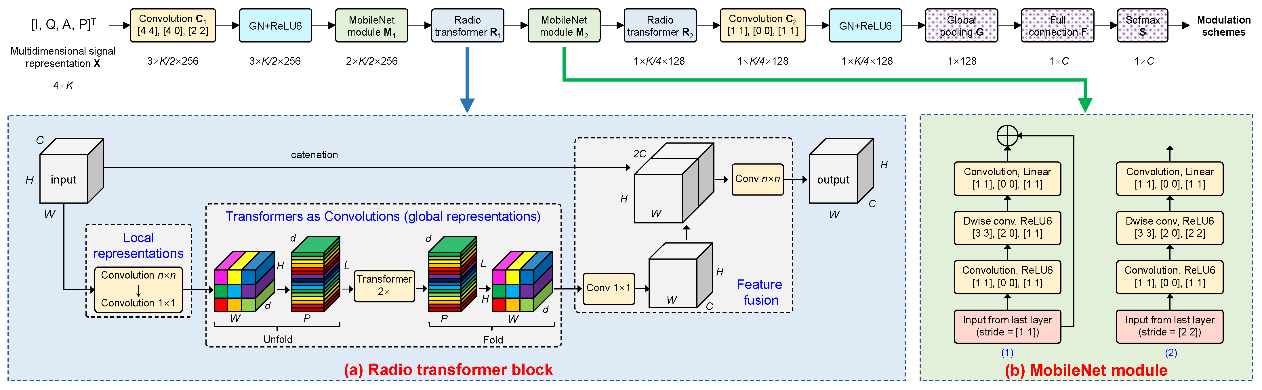
4. Lightweight Transformer MobileRaT

4.1. Model Structure

As shown in Figure 3, the proposed lightweight deep learning model, MobileRaT, consists of the following parts: two convolutional layers, C₁ and C₂; two MobileNet modules, M₁ and M₂; two radio transformer blocks, R₁ and R₂; one global pooling layer, G; one fully connected layer, F; and one softmax layer, S, for outputting AMC results.

Figure 3. Specific structure of MobileRaT.

The initial two-dimensional convolutional layer, C₁, is designed to extract the low-level features of signals and to realize the information interaction between channels I/Q and A/P. The convolutional layer, C₂, which is at the later position of the network, is used to encode high-level features and complete the fusion of features and their mapping to labels. In each convolutional layer, the size, padding, and stride of the convolution kernels are presented in detail; e.g., ([4 4], [4 0], [2 2]) a 4 × 4 size, two paddings up and down horizontally, and two strides in both the horizontal and vertical directions. In this case, the first horizontal sliding of convolutional kernels analyzes the I/Q information, the third horizontal sliding analyzes the A/P information, and the second sliding comprehensively considers the information of all four channels.

Then, the group normalization (GN) technique [48] is introduced after each convolutional layer to help accelerate the convergence of the model’s objective function during the training process, as defined by

$$G{N}_{\gamma ,\hspace{0.17em}\beta }(x_i)=\gamma \cdot \frac{x_i-{\mu }_{GN}}{\sqrt{{\sigma }_{GN}^2+\epsilon }}+\beta$$

(9)

where

$${\mu }_{GN}=\frac{1}{(C/G)HW}{\displaystyle \sum _{i=1}^{C/G}{\displaystyle \sum _{j=1}^H{\displaystyle \sum _{k=1}^W{x}_i(i,\hspace{0.17em}j,\hspace{0.17em}k)}}}$$

(10)

$${\sigma }_{GN}^2=\frac{1}{(C/G)HW}{\displaystyle \sum _{i=1}^{C/G}{\displaystyle \sum _{j=1}^H{\displaystyle \sum _{k=1}^W{(x_i(i,\hspace{0.17em}j,\hspace{0.17em}k)-{\mu }_{GN})}^2}+\epsilon }}$$

(11)

where x is the output from the last layer, and γ and β are trainable scaling scales and offsets, respectively. ε is a small constant to maintain numerical stability. In the mean value, μ, and variance, σ², H, W, C, and G represent the height, width, number of channels, and number of groups, respectively, and C/G represents the number of channels in a group. It is worth noting that G is a hyper-parameter that needs to be manually set. Although GN may bring more computation in each epoch, it usually helps the model to converge in fewer training epochs compared with batch normalization (BN) operations. Generally, GN offers higher training efficiency than BN.

To extract robust features through the nonlinear transformation of outputs after the GN operation, ReLU6 [49] is adopted as the activation function given its efficiency and adaptability, and it can be computed using

$$\mathrm{Re}\mathrm{LU}6(x)=\min (\max (0,\hspace{0.17em}x),\hspace{0.17em}6)\in [0,\hspace{0.17em}6]$$

(12)

It can be observed that, as a variant of the ReLU activation function, the ReLU6 function has the advantage of preventing the gradient from disappearing or exploding, and crucially, it possesses more efficient computation. Keeping ReLU bounded by a maximum value of six results in integers occupying up to three bits in ReLU6, leaving five bits for the decimal part. Therefore, ReLU6 is more suitable for applications in lightweight neural network models.

After the convolutional layer with GN and the activation function, the initially encoded features are further fed into the MobileNet module [50] to learn complex and abstract expert knowledge. In MobileNet modules, inputs with different resolutions from the last layer correspond to different processing methods; i.e., low-resolution feature maps in (b)-(2) are only convolved by three times, while high-resolution feature maps in (b)-(1) are still output to the next layer. In theory, the expert knowledge can be distilled without a loss of information. Firstly, the point-wise convolution (PC) [51] of size 1 × 1 is applied to the input from the last layer. Then, the depth-wise separable convolutions (DCs) [52] of size 3 × 3 are introduced to replace traditional convolutions to accelerate the forward propagation process of deep learning. As shown in Figure 4, DC acts on each channel to encode local representations and can be computed by

$$x_{i+1,\hspace{0.17em}j,\hspace{0.17em}l}=x_{i,\hspace{0.17em}j,\hspace{0.17em}l}\ast {\theta }_{i,\hspace{0.17em}j,\hspace{0.17em}l}$$

(13)

where x_{i, j, l} and θ_{i, j, l} represent the i-th channel of the j-th input feature map and corresponding weights of convolution kernels at the l-th layer, respectively. The DC operations separate the convolution and combination as two stages, which can significantly improve computation efficiency by almost a square level. The computational costs of 3 × 3 DC operations are nearly nine times smaller than those of standard convolutions.

Figure 4. Illustration of different convolution methods. (a) Standard convolution. (b) Depth-wise convolution. (c) Point-wise convolution.

Then, two radio transformer blocks are constructed to converge both local and global features in the input tensors using fewer weights than the original transformers. A combination of a 3 × 3 DC layer and a 1 × 1 DC layer is designed to extract high-dimensional representations as local features, x_L. To enable radio transformer blocks to learn global representations with spatial inductive bias, the local features are unfolded into P = WH/wh non-overlapping flattened patches, x_P, with size, w, and h. For each patch, the relationships between different patches are modeled by applying transformers, as represented by

$$x_G=\mathrm{Transformer}(x_P)$$

(14)

The transformer with the attention mechanism can be carried out according to

$$\mathrm{Attention}(Q,\hspace{0.17em}K,\hspace{0.17em}V)=\mathrm{Softmax}(\frac{Q^{T}K}{\sqrt{d_k}})V$$

(15)

where Q, K, and V are matrices of the query, keys, and values, respectively. d_k denotes the dimension of the keys. Unlike the initial transformer, which loses the spatial order of pixels, the radio transformer block neither loses the patch order nor the spatial order of pixels within each patch. Therefore, x_G can be folded and projected into the low-dimensional space using the 1 × 1 PC operation and combined with the original input, x, via concatenation. Finally, another 3 × 3 DC operation is used to fuse and encode cascaded features as outputs.

After successively stacking the above blocks, the abstract features are encoded through the global pooling layer and the fully connected layer, and the one-hot label represented by the maximum posteriori probability output from the softmax layer can be regarded as the AMC result.

4.2. Weight Evaluation

To further reduce the memory consumption of MobileRaT and speed up its inference, we establish an importance evaluation criterion for weights and gradually remove the redundant weights during the iterative training of the model based on this criterion. In this way, the establishment of the optimal sparse deep learning model structure can be transformed into a weight-solving problem under the joint constraints of the weight importance measurement and AMC accuracy.

According to information theory, information entropy measures the uncertainty and randomness of informants. During the model pre-training process, the information entropy of the same layer tends to stabilize with iterations, while the proportional relationship of information entropy in different layers gradually changes. Therefore, information entropy can be used to evaluate the importance of weights. For the weights, θ_i, at the l-th layer, their information entropy is defined as

$$\gamma ({\theta }_l)=-{\displaystyle \sum _{s=1}^S{p}_s^l{\log }_2{p}_s^l}$$

(16)

where p_s represents the probability that the weights belong to the s-th interval, in which a total of S intervals is divided. Higher information entropy indicates less variation and less information contained in the weights at this layer, and more redundant weights can thus be removed.

To better measure the information volume across different layers of the model and enable quantitative analysis of the information entropy of each layer simultaneously, the total information entropy range, IER, is expanded from

$$IER=[SIE,\hspace{0.17em}BIE]$$

(17)

to

$$IER=[SIE-{\delta }_{\max }(BIE-SIE),\hspace{0.17em}BIE+{\delta }_{\max }(BIE-SIE)]$$

(18)

where SIE and BIE are the minimum and maximum values of information entropy in each layer of the network model. δ_max ∈ [δ₁, δ₂, …, δ_L] represents the maximum pruning rate of weights, where L is the number of total learnable layers in the model. By dividing the information entropy range, IER, of the model into 10 equal parts, each of which is denoted by IER_δ, the weight-pruning rate of each layer in the neural network model can be calculated as

$${\delta }_l=\lceil \gamma ({\theta }_l)\in IE{R}_{\delta }\rceil$$

(19)

where $\lceil \cdot \rceil$ means taking the smallest integer that is greater than or equal to the result within the symbol. It is worth noting that the importance evaluation object is the weights rather than the convolutional kernels, which facilitate the construction of sparse structures and maintain the parameter space from large models. As a result, weights as pruning objects usually possess a more promising capacity in terms of generalization capabilities than convolutional kernels while also improving inference efficiency.

The importance evaluation of learnable weights in MobileNet and the evolution process of IER are presented in Figure 5. The flexible information entropy range, IER, can adapt to training iterations that contain different mini-batch samples, avoiding excessive weights being removed, as the pruning and learning process is irreversible. Once the model structure is destroyed, the achieved AMC performance cannot be restored. Hence, iterative learning is chosen to conservatively and gradually remove redundant weights.

Figure 5. Evolution process of the information entropy range, IER.

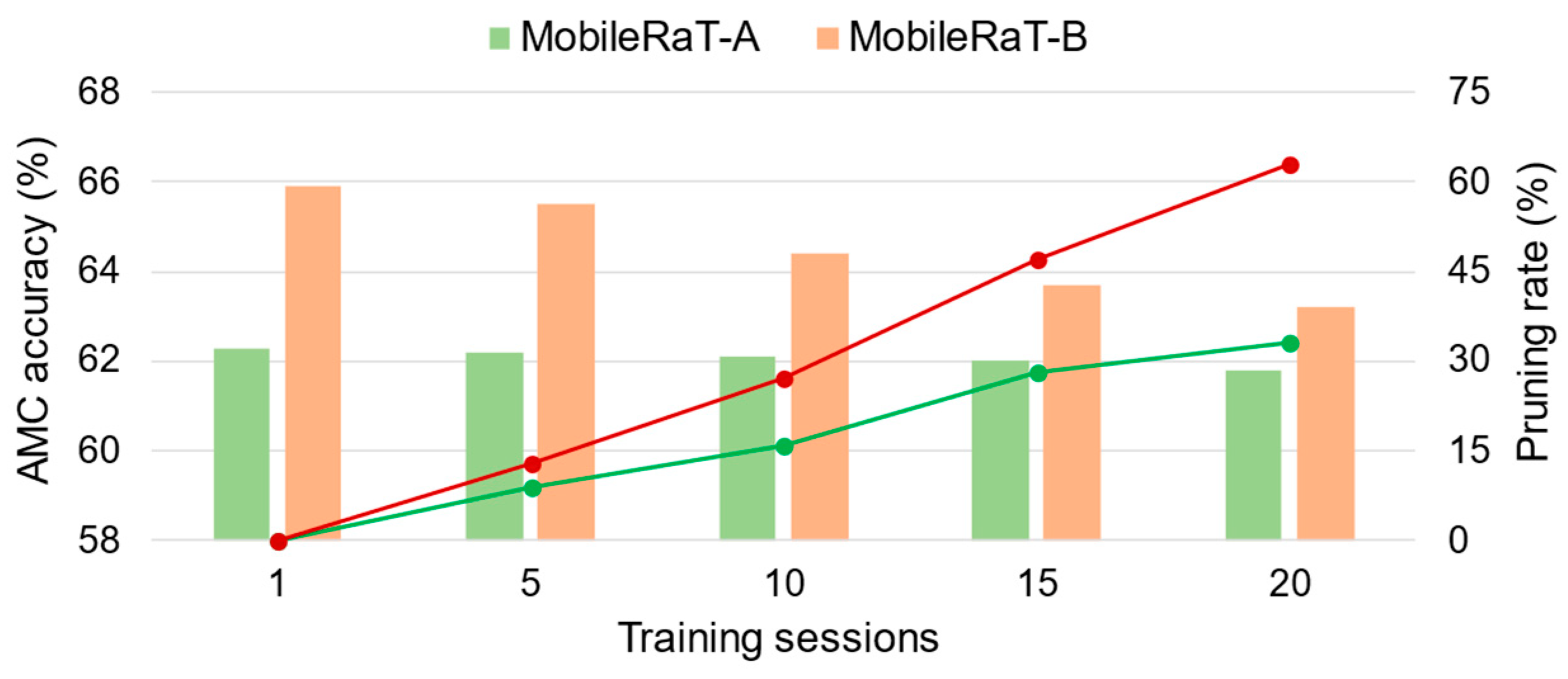
4.3. Iterative Learning

The constructed deep learning model, MobileRaT, needs to be trained to learn key knowledge from signal representation and is then used for AMC. During the iterative learning process of the model, weights can be simultaneously updated and pruned in search of an ideal lightweight structure accompanied by excellent AMC performance. Considering that multiple training sessions need to be repeated to remove and finetune the weights, a back-propagation-based stochastic gradient descent (SGD) with warm restart is used to update the parameters, as represented by

$${\theta }^{t+1}={\theta }^t+v^{t+1}$$

(20)

$$v^{t+1}={\mu }^t{v}^t-{\alpha }^t\nabla {ℒ}^t({\theta }^t)$$

(21)

in which the cross-entropy loss, $ℒ$, is defined as

$${ℒ}^t=-{\displaystyle \sum _{m=1}^M{\mathbf{Y}}_m{\left[\log ({\mathbf{M}}^t(\mathbf{X}))\right]}_m}$$

(22)

In the above equations, v^t is a velocity vector at the t-th training iteration; µ^t is a momentum rate that defines a trade-off between current and past observations of the gradients, ∇$ℒ$^t; and α^t represents the decreasing learning rate with a warm restart. Within the i-th training session, the learning rate is decayed in a cosine-annealing manner for each mini-batch set, as represented by

$${\alpha }^t={\alpha }_{\min }^i+\frac{1}{2}({\alpha }_{\max }^i-{\alpha }_{\min }^i)(1+\cos (\frac{T_{cur}}{T_i}\pi ))$$

(23)

where α_min and α_max are ranges for the learning rate, T_i is the current number of training epochs, and T_cur accounts for the number of training epochs that have been performed since the last restart. Equations (20)–(23) are repeated until the change in the objective function over a period of epochs is less than the threshold or reaching the required maximum number of epochs, and thus the model is considered to have found a suitable minimum location. At this point, a model training session is regarded as finished.

When a training session is completed, i.e., after the model’s objective function converges, the importance of the weights is evaluated, and redundant ones are removed. Then, the smaller learning rate is initialized for the next round of SGD optimization. The objective function is optimized iteratively until the model satisfies the trade-off between AMC accuracy and the overall pruning rate. The pseudo-code of the whole iterative learning algorithm is summarized in Algorithm 1.

Algorithm 1. Iterative learning process of MobileRaT.

Input: training set and validation set.

Initialization: deep learning model and hyper-parameters.

1:    for each training session do

2:        for each training iteration do

3:            forward propagation: loss computation as Equation (22).

4:            back-propagation: weights update as Equation (20).

5:        end for

6:        learning rate update as Equation (23).

7:        weights removal according to Equation (19).

8:    until the trade-off satisfies the condition

Output: the convergent lightweight deep learning model.

5. Experimental Results and Analysis

In this section, we perform extensive experiments and analyses. A series of state-of-the-art methods are compared to demonstrate the superior performance of the proposed method, and ablation experiments are also conducted to observe the robustness of MobileRaT.

5.1. Experimental Settings

5.1.1. Experimental Dataset

During the experiments, two datasets of different scales (i.e., RadioML 2018.01A [36] and RadioML 2016.10A [37]) are used for AMC performance evaluations of deep learning models at workstations and edge computing devices, respectively. The dataset RadioML 2018.01A [36] contains a total of two million I/Q signals covering 24 modulation schemes {OOK, 4ASK, 8ASK, BPSK, QPSK, 8PSK, 16PSK, 32PSK, 16APSK, 32APSK, 64APSK, 128APSK, 16QAM, 32QAM, 64QAM, 128QAM, 256QAM, AM-SSB-WC, AM-SSB-SC, AM-DSB-WC, AM-DSB-SC, FM, GMSK, OQPSK} with a signal size of 2 × 1024. RadioML 2016.10A [37] consists of 220,000 signals with 11 modulation schemes of size 2 × 128, including {BPSK, QPSK, 8PSK, QAM16, QAM64, GFSK, CPFSK, PAM4, AM-DSB, AM-SSB, WBFM).

All the experimental wireless communication signals are generated in a realistic environment with the introduction of carried data (e.g., real speech and text) and other transmission parameters consistent with real environmental conditions. Real speech and text are modulated onto the signal, and the data are whitened using a block randomizer to ensure that the bits are proportional. Then, unknown scaling, translation, expansion, and impulse noise are considered in the challenging channel model. Finally, the transmission signals are generated using channel model blocks in GNU Radio [53]. These modulated signals, with a 1 MHz bandwidth and SNRs ranging from −20 dB to +18 dB, are uniformly distributed in each category.

During the experiments, the number of samples in the training, validation, and test sets is divided in a ratio of 6:2:2. The training and validation sets are used to optimize the weights and structure and help determine appropriate hyper-parameters, respectively, and the test set is used to evaluate the convergent lightweight model.

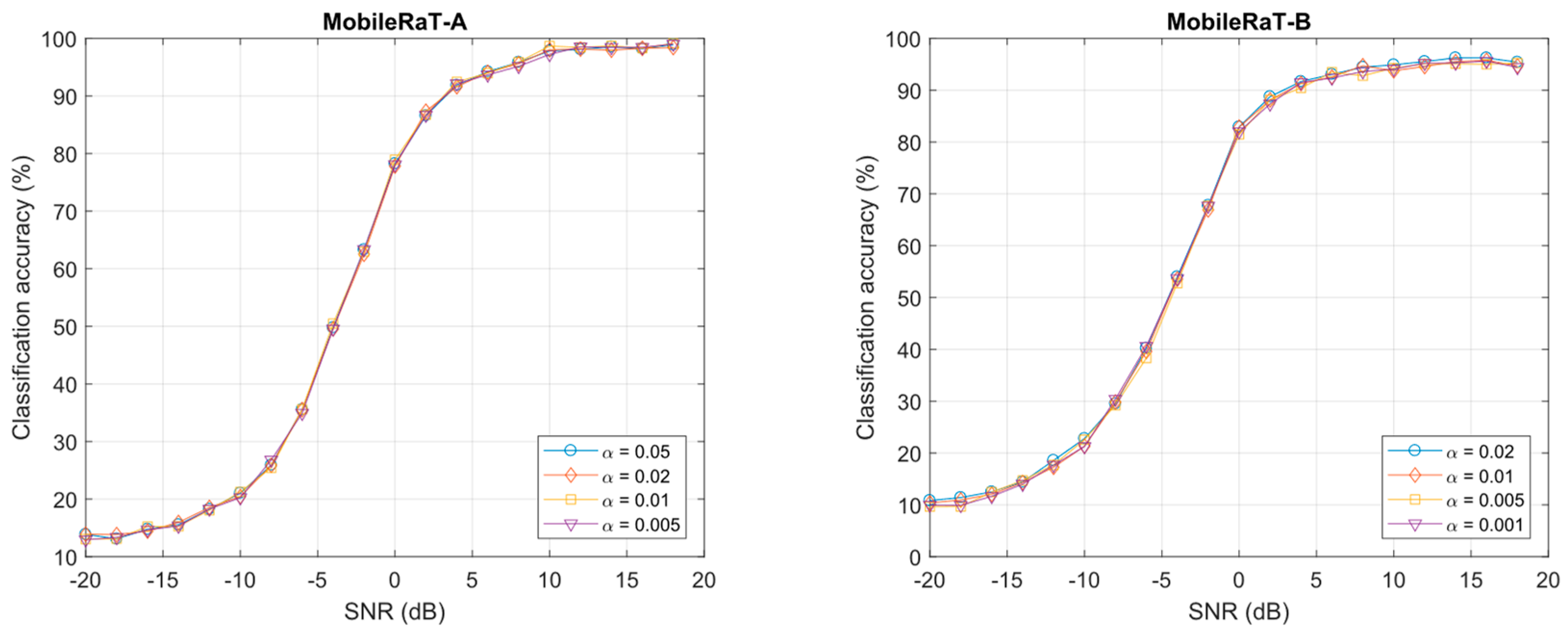
5.1.2. Hyper-Parameter Setting

For two experimental datasets with different scales, two models, MobileRaT-A and MobileRaT-B, with different settings are trained and pruned, respectively, to meet the requirements of workstations and edge devices. All the hyper-parameters during the training and testing process, including the learning rate, momentum rate, batch size, weight decay rate, small constant, pruning rate, and accuracy loss, are summarized in Table 1. It can be seen that MobileRaT-A, which deals with the large dataset, RadioML 2018.01A, uses generally large hyper-parameters to help explore the broad loss plane and find suitable convergent locations. By contrast, MobileRaT-B, which deals with the smaller dataset, RadioML 2016.10A, adopts a more conservative hyper-parameter setting to seek a stable convergence position. In addition, MobileRaT-B adopts a strict pruning rate (60%) but a loose accuracy loss (5%) to search for lightweight structures that can be easily deployed in an edge device.

Table 1. Hyper-parameter settings in MobileRaT.

Hyper-Parameters	MobileRaT-A	MobileRaT-B
learning rate	0.05	0.01
momentum rate	0.9	0.9
batch size	128	64
weight decay rate	0.0005	0.0005
small constant	10−5	10−5
pruning rate	>30%	>60%
accuracy loss	<3%	<5%

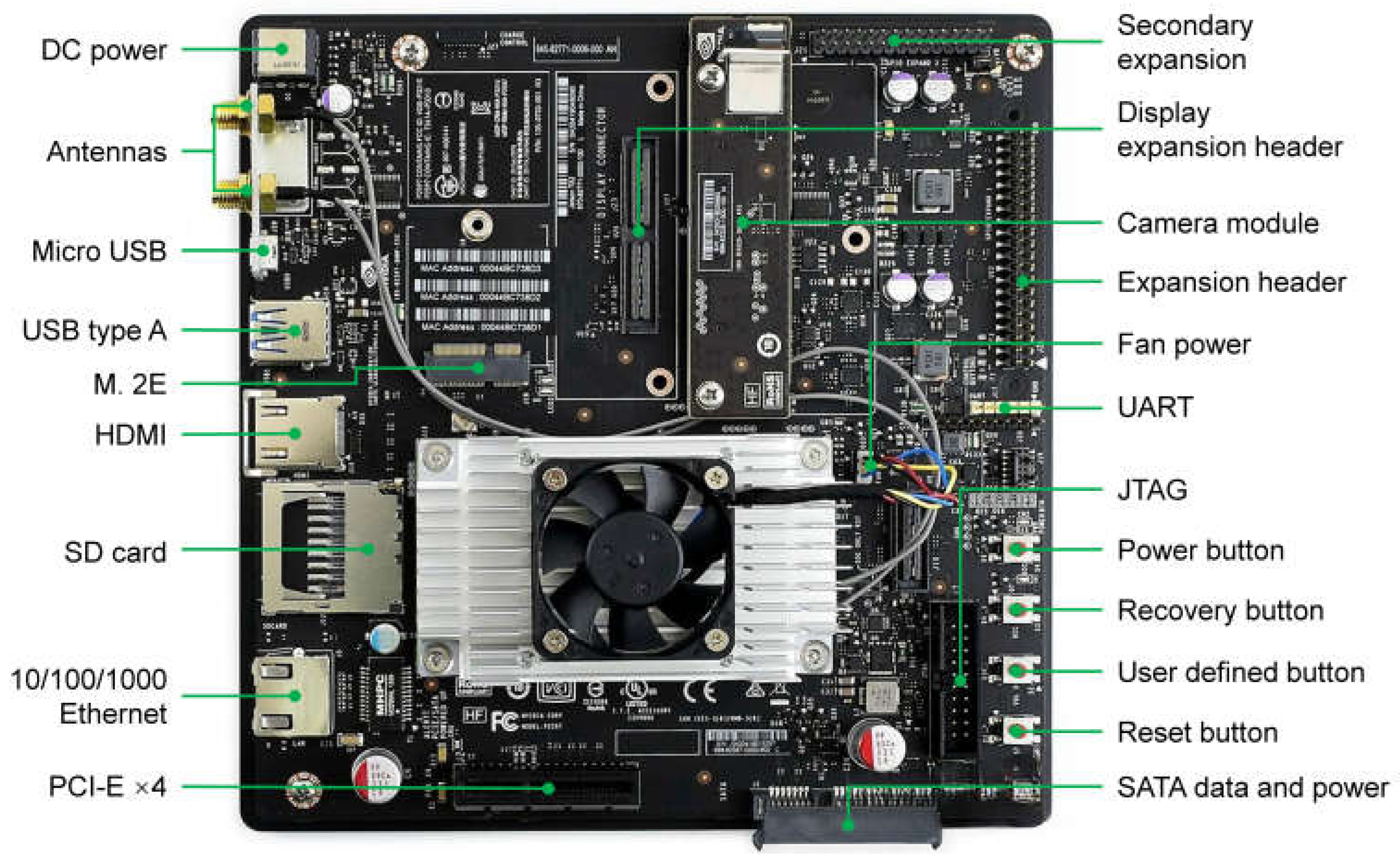
5.1.3. Implementation Platform

Both MobileRaT-A and MobileRaT-B are trained using the PyTorch framework, based on a workstation consisting of an Intel(R) Core(TM) i9-12900KS CPU, an NVIDIA RTX 3090 GPU, 2 × 16 GB RAM, and a 1 TB SSD. In the AMC performance evaluation phase, MobileRaT-A is tested on the workstation while MobileRaT-B is tested on the edge device, an NVIDIA Jetson TX2, which integrates a 256-core NVIDIA Pascal GPU, 6-core 64-bit ARMv8 cortex-A57 CPU clusters, and 8 GB of DDR4 RAM, as shown in Figure 6. The Jetson TX2 measures 50 × 87 mm, weighs 85 g, and has a standard power of 7.5 W. The workstation side focuses on the AMC accuracy of MobileRaT, while the edge side takes into account both AMC accuracy and real-time requirements.

Figure 6. Hardware structure of edge computing platform Jetson TX2.

5.1.4. Evaluation Metrics

For AMC performance evaluation, three metrics, including accuracy, memory footprint (characterized by the number of parameters), and inference speed are counted in the testing stage. AMC accuracy places demands on the inference ability of the model, while memory footprint and inference speed verify the practical application possibilities with limited power and computational capacity.

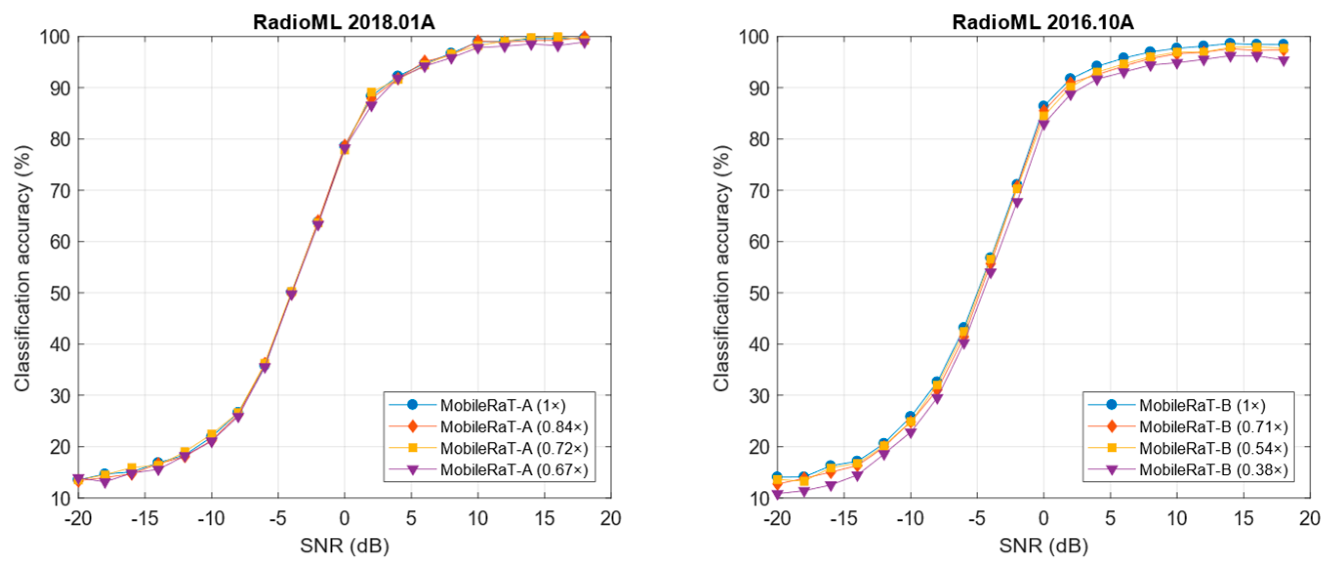
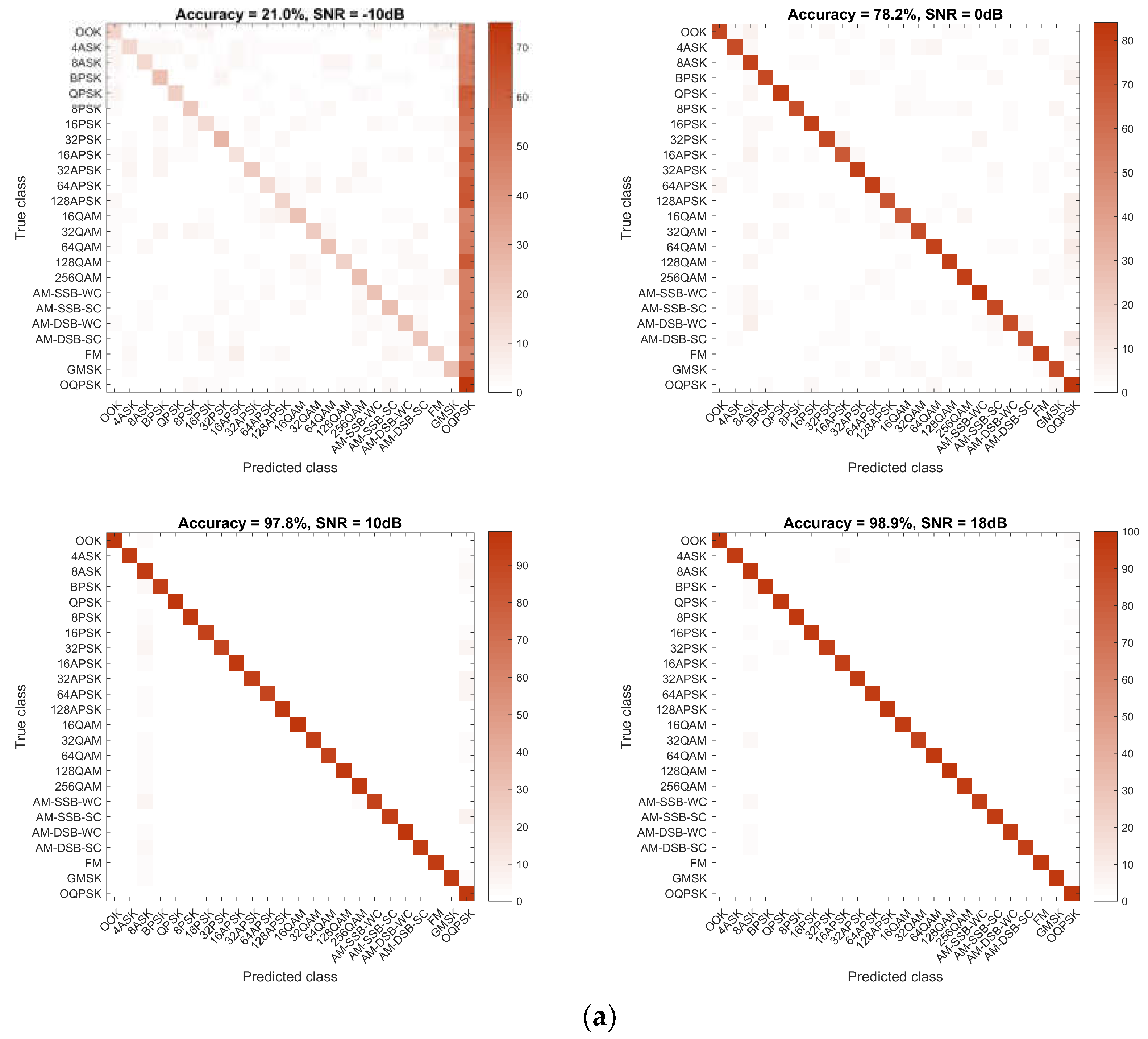
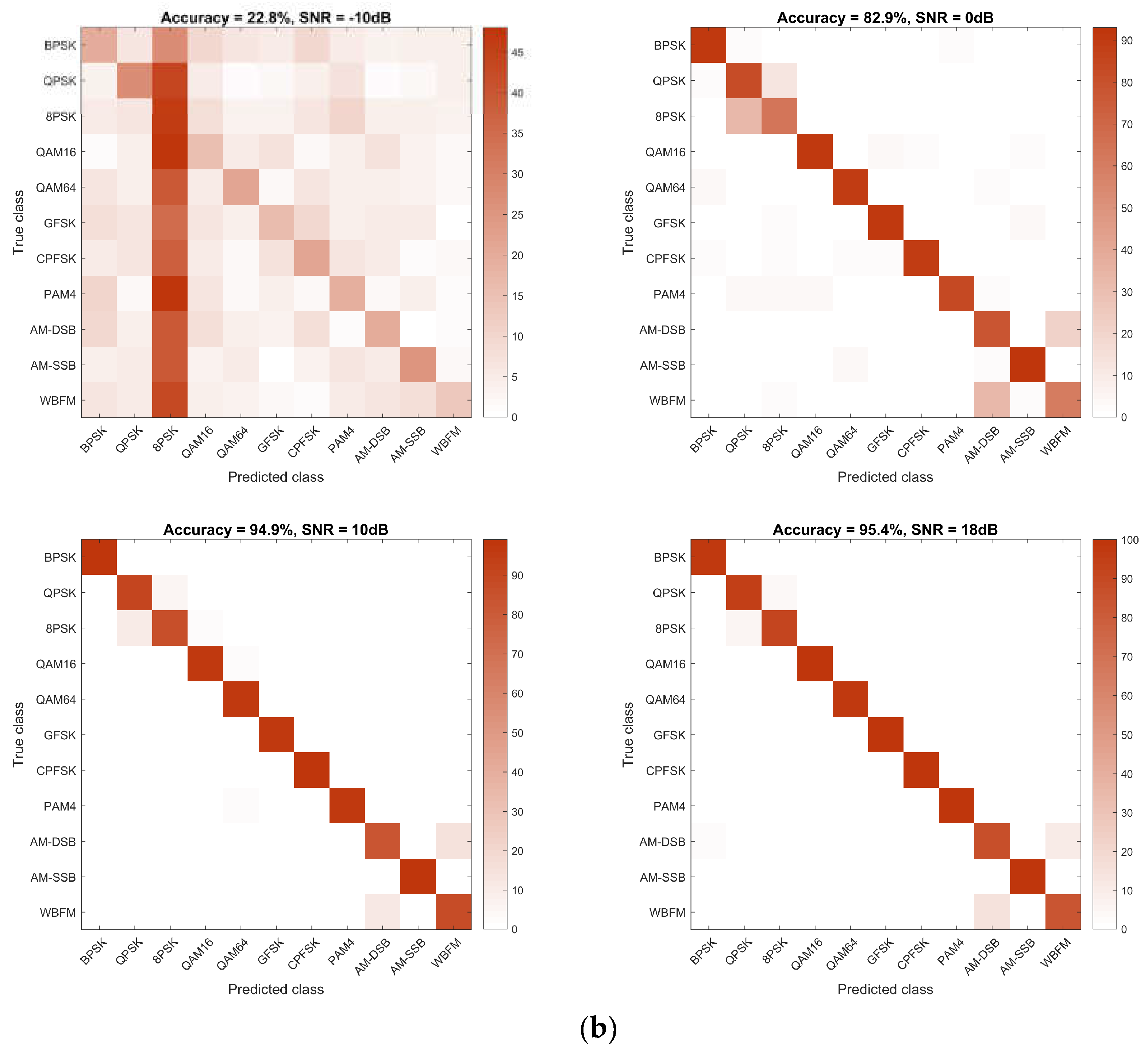
5.2. AMC Performance of MobileRaT

In Table 2, we report the AMC performance of MobileRaTs on the training, validation, and test sets, including the model accuracy, number of parameters, and inference speed for a different number of training sessions. The pruned models that iterated to the end, i.e., MobileRaT-A and MobileRaT-B, are only 67% and 38% of the original size, respectively. The AMC accuracy of the pruned models in the training and validation sets is decreased slightly (2.4%↓ and 0.3%↓ in MobileRaT-A, 4.1%↓ and 1.5%↓ in MobileRaT-B) to prevent overfitting with fewer parameters. The accuracy losses of MobileRaT-A and MobileRaT-B in the test set are no more than 0.5% and 2.7% respectively, while the number of parameters is reduced by 89 k and 166 k, respectively, which allows the inference speed to meet the requirements of real-time signal analysis with negligible accuracy loss. The accuracy loss in MobileRaT-B was more pronounced than in MobileRaT-A because of its larger pruning rate and the difficulty of learning features from signals of shorter lengths. The average test accuracies of MobileRaT-A and MobileRaT-B after pruning reached 61.8% and 63.2%, respectively, mainly affected by signals with low SNRs. In terms of generalization errors, the generalization gap between the validation accuracy and test accuracy of both models is less than 4%, demonstrating training efficiency.

Table 2. AMC performance of MobileRaT with RadioML 2018.01A and RadioML 2016.10A.

Evaluation Metrics	MobileRaT-A (1×)	MobileRaT-A (0.67×)	MobileRaT-B (1×)	MobileRaT-B (0.38×)
Training accuracy (%)	74.6	72.2	78.8	74.7
Validation accuracy (%)	65.3	65.0	68.7	67.2
Testing accuracy (%)	62.3	61.8	65.9	63.2
Number of weights (k)	271	182	268	102
Inference speed (ms)	1.3	0.9	7.6	4.4

Then, we observe the AMC accuracy of the model under different SNRs, as shown in Figure 7. The MobileNet-A model trained on the large-scale dataset is robust to the number of parameters, and models of different sizes exhibit approximate test accuracies. MobileRaT-A shows a classification accuracy of nearly 80% for distinguishing 24 types of modulation schemes at 0 dB. The parameter size of MobileRaT-B demonstrates a more pronounced impact on the AMC accuracy, especially at low SNRs. When SNR > 0 dB, MobileRaT-B achieves an overall AMC accuracy that is > 90%. Affected by the number of sampling points, both MobileRaT-A and MobileRaT-B exhibit limited AMC performance (about 10%) at extremely low SNRs, e.g., −20 dB. On the other hand, it is difficult for the model to achieve 100% accuracy even at high SNRs because the feature learning is also influenced by other parameters like symbol rate, sampling frequency, and signal attenuation caused by multipath propagation.

Figure 7. AMC accuracy of MobileRaT under different SNRs.

To further observe the classification performance of various modulation schemes, the confusion matrices for representative SNR conditions (−10 dB, 0 dB, 10 dB, 18 dB) are visualized in Figure 8. At low SNRs, the model tends to recognize all modulations as a specific one or several because of its inability to learn sufficient features. For example, MobileRaT-A recognized most samples as 8ASK or OQPSK modulations with an accuracy of 21.0% at −10 dB. Similarly, MobileRaT-B identified a large number of samples as 8PSK with an accuracy of 22.8% at −10 dB. As the SNR increases, the modulation schemes of the samples can be gradually distinguished. When SNRs are > 0, almost all the modulation schemes can be effectively distinguished by MobileRaT-A with an accuracy of >78.2%, except for QPSK/8PSK and AM-DSB/WBFM in MobileRaT-B. 8PSK symbols containing specific bits are indistinguishable from QPSK because QPSK constellation points are sampled from 8PSK points, which usually requires the construction of a multilevel model or the raising of sampling points like RadioML 2018.01A. When distinguishing between AM-DSB and WBFM, the analog speech signals have periods of silence with only carrier tones, making these samples unrecognizable but not detrimental to the actual task.

Figure 8. Confusion matrices of MobileRaT under representative SNRs. (a) MobileRaT-A. (b) MobileRaT-B.

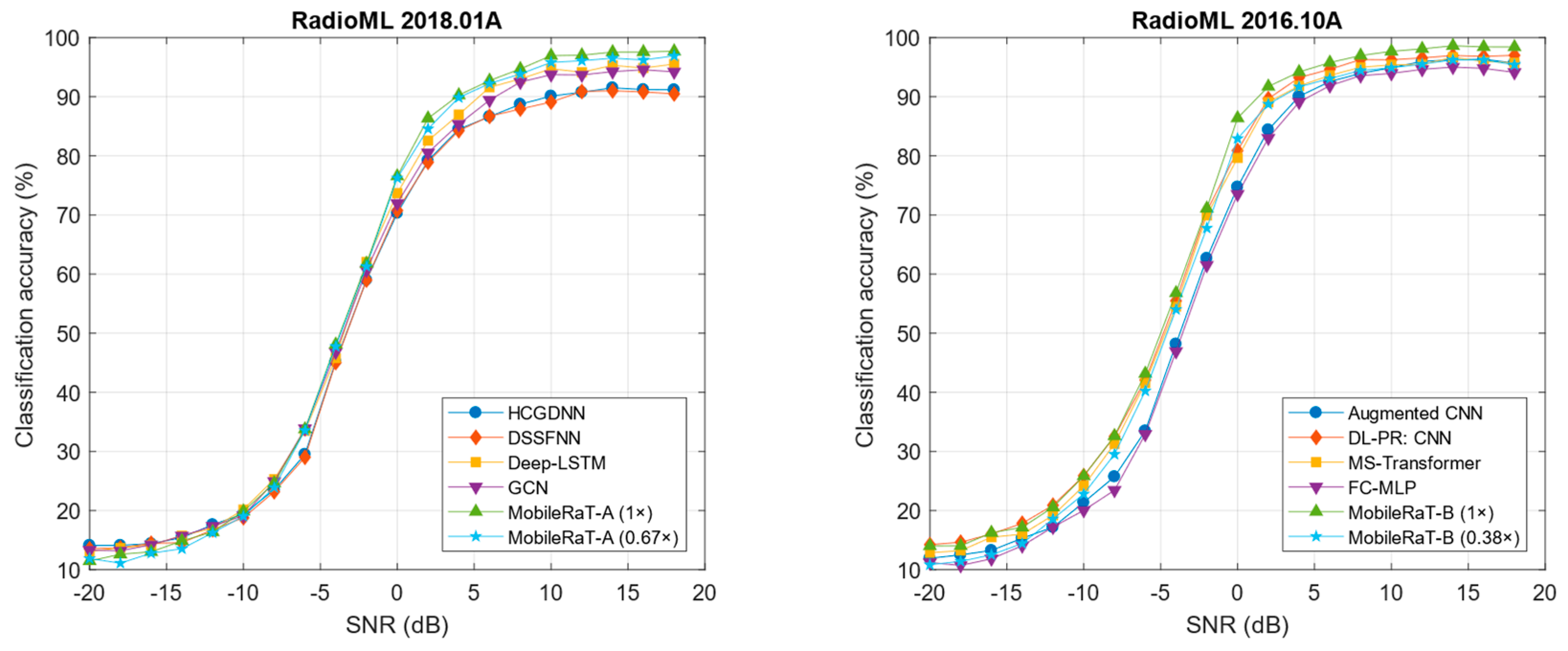
5.3. Comparison with State-of-the-Art Methods

In this part, a series of state-of-the-art methods is compared to prove the superiority of the proposed method, and the experimental results of two datasets are reported in Table 3 and Table 4. The experimental results for the larger dataset, RadioML 2018.01A, are mainly observed to determine the AMC accuracy by comparing it with HCGDNN [5], DSSFNN [13], Deep-LSTM [29], and GCN [31], while the smaller dataset, RadioML 2016.10A, is tested to comprehensively evaluate the overall AMC performance by comparing it with Augmented CNN [27], DL-PR: CNN [30], MS-Transformer [32], and FC-MLP [46]. According to the results, the pruned models, i.e., MobileRaT-A (0.67×) and MobileRaT-B (0.38×), improve their respective AMC accuracies from 60.2% and 62.6% to 61.8% and 63.2%, accompanied by more efficient reasoning. Even on the edge device, Jetson TX2, MobileRaT-B shows a real-time reasoning speed of 4.4 ms per signal, which is able to meet the communication latency requirements of the IEEE 802.16m protocol. Moreover, MobileRaT-A, with a parameter quantity of 182 k, and MobileRaT-B, with 102 k parameters, can be easily deployed in the receiver, helping to construct an intelligent and efficient drone communication system.

Table 3. Comparison of MobileRaT-A and state-of-the-art methods with RadioML 2018.01A.

Methods	AMC Accuracy (%)	Number of Weights (k)	Inference Speed (ms)
HCGDNN [5]	57.9	242	1.4
DSSFNN [13]	57.4	608	4.3
Deep-LSTM [29]	60.2	565	9.8
GCN [31]	59.6	442	7.5
MobileRaT-A (1×)	62.3	271	1.3
MobileRaT-A (0.84×)	62.1	228	1.2
MobileRaT-A (0.72×)	62.0	195	1.2
MobileRaT-A (0.67×)	61.8	182	0.9

Table 4. Comparison of MobileRaT-B and state-of-the-art methods with RadioML 2016.10A.

Methods	AMC Accuracy (%)	Number of Weights (k)	Inference Speed (ms)
Augmented CNN [27]	58.8	92	3.2
DL-PR: CNN [30]	62.6	224	7.9
MS-Transformer [32]	61.4	220	9.0
FC-MLP [46]	57.6	170	6.8
MobileRaT-B (1×)	65.9	268	7.6
MobileRaT-B (0.71×)	64.4	190	7.1
MobileRaT-B (0.54×)	63.7	145	5.9
MobileRaT-B (0.38×)	63.2	102	4.4

In Figure 9, we report the AMC accuracy of various methods under different SNRs. It can be clearly seen that the AMC accuracies of all methods are similar under low SNRs, while the superiority of the proposed MobileRaT under high SNRs can be demonstrated. When SNR > 0 dB, both the original MobileRaT-A (1×) and the pruned MobileRaT-A (0.67×) exhibit good AMC accuracy for all SNRs. The results for MobileRaT-B are more obvious, showing a competitive accuracy advantage in SNRs > −10 dB. As for the compared methods, both CNN [5,13,30] and GCN [31] show competitive accuracy compared with LSTM [29] in AMC tasks driven by samples of different sizes but with more efficient inference performance. The conventional dense connected model, i.e., FC-MLP [46], is limited in handling small-scale samples in RadioML 2016.10A since the generalization performance of dense parameters is easily affected.

Figure 9. Comparison of the AMC accuracy of the state-of-the-art methods under different SNRs.

5.4. Robustness Analysis

The robustness of a model to hyper-parameters determines its generalization ability across different scenarios in practical applications. Therefore, we report the AMC accuracy of MobileRaT under different hyper-parameters, including the initial learning rate and batch size, as shown in Figure 10. The learning rate is related to the whole iterative process of the model by influencing the optimization step size. The batch size affects the optimization direction by determining the batch gradient. If a deep learning model is sensitive to the learning rate and batch size, it struggles to adapt to different communication scenarios. According to the results, the variation in the model’s AMC accuracy with different hyper-parameter settings is less than 1% and negligible. The experimental results demonstrate the robustness of MobileRaT to hyper-parameters, indicating that the model can adapt to complex and ever-changing drone communication environments.

Figure 10. Impact of hyper-parameters on the AMC accuracy of MobileRaT.

The impact of signal representations, including I/Q, A/P, and I/Q/A/P, on the AMC accuracy of MobileRaT is reported in Table 5. It shows that signal representations that aggregate multimodal information achieve the best AMC accuracy, improving the accuracy from 60.6% (I/Q)/59.4% (A/P) and 61.8% (I/Q)/60.8% (A/P) to 61.8% (I/Q/A/P) and 63.2% (I/Q/A/P) in MobileRaT-A and MobileRaT-B, respectively. On the other hand, I/Q mode usually performs better than A/P mode, as I/Q mode covers A/P information while A/P mode loses some of the frequency domain information. However, it is worth noting that single modality is not as sensitive to changes in parameter scales as multimodality (the accuracy loss is less than 1.5% from 1× to 0.67× in MobileRaT-A, and the accuracy loss is less than 3% from 1× to 0.38× in MobileRaT-B), possibly because more parameters are required for more implicit expert knowledge, which is unfavorable for real-time edge computing.

Table 5. Impact of signal representations on the AMC accuracy of MobileRaT.

Models	[I Q]T	[A P]T	[I Q A P]T
MobileRaT-A (1×)	61.2	60.8	62.3
MobileRaT-A (0.84×)	60.9	60.4	62.1
MobileRaT-A (0.72×)	60.7	60.1	62.0
MobileRaT-A (0.67×)	60.6	59.4	61.8
MobileRaT-B (1×)	63.9	61.8	65.9
MobileRaT-B (0.71×)	62.7	61.1	64.4
MobileRaT-B (0.54×)	62.2	60.6	63.7
MobileRaT-B (0.38×)	61.8	60.8	63.2

Furthermore, we observe the relationship between AMC accuracy and the pruning rate of MobileRaT, as shown in Figure 11. As the training session increases, more weights are removed from the model, resulting in a certain degree of decrease in the AMC accuracy of the model. The accuracy loss (2.7%↓) of MobileRaT-B deployed in the edge device is more obvious than MobileRaT-A because of its strict pruning rate requirements (>60%). In the 15th training session, MobileRaT-B removes nearly half of the weights with only about 2% AMC accuracy loss. The accuracy loss of MobileRaT-A is less than 1% after removing more than 30% of the weights. Overall, the improvement in the inference efficiency due to redundant parameters removal is encouraging compared with the slight accuracy loss. In other words, deploying a pruned lightweight deep learning model in the edge device is feasible.

Figure 11. The relationship between AMC accuracy and the pruning rate.

6. Conclusions

AMC has become a key component of next-generation drone communication systems, which are crucial for improving non-cooperative communication efficiency. In this paper, we propose a real-time AMC method based on the lightweight deep learning model MobileRaT. The constructed radio transformer is trained iteratively accompanied by weight pruning in order to learn robust modulation knowledge from multimodal signal representations for AMC. To the best of our knowledge, this is the first attempt in which the pruning technique and a lightweight transformer model are integrated and applied to the processing of temporal signals, ensuring AMC accuracy while also improving its inference efficiency. MobileRaT-A and MobileRaT-B of different scales are deployed in a workstation and an edge device and tested and compared using RadioML 2018.01A and Radio 2016.10A, respectively. In the experimental process, we considered complex communication interference factors, including channel gain, frequency offset, phase offset, and Gaussian noise. The experimental results of comparisons with a series of state-of-the-art methods confirm the superiority of MobileRaT. Furthermore, ablation studies are conducted to demonstrate the robustness of MobileRaT to hyper-parameters (initial learning rate and batch size) and signal representations ([I Q]^T, [A P]^T, and [I Q A P]^T). In conclusion, the lightweight deep learning model based on redundant weight removal improves the realistic possibility of applying AMC to drone communication systems.

In the future, we plan to conduct practical communication testing and verification through the deployment of deep learning models mounted on drones. By studying the introduction and utilization of prior information, we aim to improve the generalization capability of deep learning models under various communication conditions, such as the channel fading effect, symbol rate, sampling rate, roll-off factor, stopband attenuation, and mixed noise. Therefore, some simulation data containing specific parameter settings can also be considered to improve the AMC accuracy of deep learning models.

References

1. Wei, M.; Sezginer, S.; Gui, G.; Sari, H. Bridging spatial modulation with spatial multiplexing: Frequency-domain ESM. IEEE J. Sel. Top. Signal Process. 2019, 13, 1326–1335. [Google Scholar] [CrossRef]
2. Ma, M.; Xu, Y.; Wang, Z.; Fu, X.; Gui, G. Decentralized learning and model averaging based automatic modulation classification in drone communication systems. Drones 2023, 7, 391. [Google Scholar] [CrossRef]
3. Zhang, H.; Zhou, F.; Wu, Q.; Wu, W.; Hu, R.Q. A novel automatic modulation classification scheme based on multi-scale networks. IEEE Trans. Cogn. Commun. Netw. 2021, 8, 97–110. [Google Scholar] [CrossRef]
4. Zheng, Q.; Wang, R.; Tian, X.; Yu, Z.; Wang, H.; Elhanashi, A.; Saponara, S. A real-time transformer discharge pattern recognition method based on CNN-LSTM driven by few-shot learning. Electr. Power Syst. Res. 2023, 219, 109241. [Google Scholar] [CrossRef]
5. Chang, S.; Zhang, R.; Ji, K.; Huang, S.; Feng, Z. A hierarchical classification head based convolutional gated deep neural network for automatic modulation classification. IEEE Trans. Wirel. Commun. 2022, 21, 8713–8728. [Google Scholar] [CrossRef]
6. Wang, Y.; Gui, G.; Gacanin, H.; Ohtsuki, T.; Dobre, O.A.; Poor, H.V. An efficient specific emitter identification method based on complex-valued neural networks and network compression. IEEE J. Sel. Areas Commun. 2021, 39, 2305–2317. [Google Scholar] [CrossRef]
7. Liu, X.; Sun, C.; Yu, W.; Zhou, M. Reinforcement-learning-based dynamic spectrum access for software-defined cognitive industrial internet of things. IEEE Trans. Ind. Inform. 2021, 18, 4244–4253. [Google Scholar] [CrossRef]
8. Dong, B.; Liu, Y.; Gui, G.; Fu, X.; Dong, H.; Adebisi, B.; Gacanin, H.; Sari, H. A lightweight decentralized-learning-based automatic modulation classification method for resource-constrained edge devices. IEEE Internet Things J. 2022, 9, 24708–24720. [Google Scholar]
9. Peng, Y.; Guo, L.; Yan, J.; Tao, M.; Fu, X.; Lin, Y.; Gui, G. Automatic modulation classification using deep residual neural network with masked modeling for wireless communications. Drones 2023, 7, 390. [Google Scholar] [CrossRef]
10. Shen, Y.; Yuan, H.; Zhang, P.; Li, Y.; Cai, M.; Li, J. A multi-subsampling self-attention network for unmanned aerial vehicle-to-ground automatic modulation recognition system. Drones 2023, 7, 376. [Google Scholar] [CrossRef]
11. Zhang, X.; Zhao, H.; Zhu, H.; Adebisi, B.; Gui, G.; Gacanin, H.; Adachi, F. NAS-AMR: Neural architecture search-based automatic modulation recognition for integrated sensing and communication systems. IEEE Trans. Cogn. Commun. Netw. 2022, 8, 1374–1386. [Google Scholar] [CrossRef]
12. Fu, X.; Gui, G.; Wang, Y.; Gacanin, H.; Adachi, F. Automatic modulation classification based on decentralized learning and ensemble learning. IEEE Trans. Veh. Technol. 2022, 71, 7942–7946. [Google Scholar] [CrossRef]
13. Gong, A.; Zhang, X.; Wang, Y.; Zhang, Y.; Li, M. Hybrid data augmentation and dual-stream spatiotemporal fusion neural network for automatic modulation classification in drone communications. Drones 2023, 7, 346. [Google Scholar] [CrossRef]
14. Fu, X.; Gui, G.; Wang, Y.; Ohtsuki, T.; Adebisi, B.; Gacanin, H.; Adachi, F. Lightweight automatic modulation classification based on decentralized learning. IEEE Trans. Cogn. Commun. Netw. 2021, 8, 57–70. [Google Scholar] [CrossRef]
15. Huan, C.Y.; Polydoros, A. Likelihood methods for MPSK modulation classification. IEEE Trans. Commun. 1995, 43, 1493–1504. [Google Scholar] [CrossRef]
16. Tadaion, A.A.; Derakhtian, M.; Gazor, S.; Aref, M.R. Likelihood ratio tests for PSK modulation classification in unknown noise environment. In Proceedings of the IEEE Canadian Conference on Electrical and Computer Engineering, Saskatoon, SK, Canada, 1–4 May 2005; pp. 151–154. [Google Scholar]
17. Panagiotou, P.; Anastasopoulos, A.; Polydoros, A. Likelihood ratio tests for modulation classification. In Proceedings of the IEEE 21st Century Military Communications. Architectures and Technologies for Information Superiority (Cat. No. 00CH37155), Los Angeles, CA, USA, 22–25 October 2000; Volume 2, pp. 670–674. [Google Scholar]
18. Xie, L.; Wan, Q. Cyclic feature based modulation recognition using compressive sensing. IEEE Wirel. Commun. Lett. 2017, 6, 402–405. [Google Scholar] [CrossRef]
19. Li, T.; Li, Y.; Dobre, O.A. Modulation classification based on fourth-order cumulants of superposed signal in NOMA systems. IEEE Trans. Inf. Forensics Secur. 2021, 16, 2885–2897. [Google Scholar] [CrossRef]
20. Carnì, D.L.; Balestrieri, E.; Tudosa, I.; Lamonaca, F. Application of machine learning techniques and empirical mode decomposition for the classification of analog modulated signals. Acta Imeko 2020, 9, 66–74. [Google Scholar] [CrossRef]
21. Wei, Y.; Fang, S.; Wang, X. Automatic modulation classification of digital communication signals using SVM based on hybrid features, cyclostationary, and information entropy. Entropy 2019, 21, 745. [Google Scholar] [CrossRef]
22. Zhao, Y.; Shi, C.; Wang, D.; Chen, X.; Wang, L.; Yang, T.; Du, J. Low-complexity and nonlinearity-tolerant modulation format identification using random forest. IEEE Photonics Technol. Lett. 2019, 31, 853–856. [Google Scholar] [CrossRef]
23. Zheng, Q.; Tian, X.; Yu, Z.; Jiang, N.; Elhanashi, A.; Saponara, S.; Yu, R. Application of wavelet-packet transform driven deep learning method in PM2.5 concentration prediction: A case study of Qingdao, China. Sustain. Cities Soc. 2023, 92, 104486. [Google Scholar] [CrossRef]
24. Zheng, Q.; Zhao, P.; Zhang, D.; Wang, H. MR-DCAE: Manifold regularization-based deep convolutional autoencoder for unauthorized broadcasting identification. Int. J. Intell. Syst. 2021, 36, 7204–7238. [Google Scholar] [CrossRef]
25. Wang, Y.; Gui, G.; Lin, Y.; Wu, H.C.; Yuen, C.; Adachi, F. Few-shot specific emitter identification via deep metric ensemble learning. IEEE Internet Things J. 2022, 9, 24980–24994. [Google Scholar] [CrossRef]
26. Zhang, Q.; Nicolson, A.; Wang, M.; Paliwal, K.K.; Wang, C. DeepMMSE: A deep learning approach to MMSE-based noise power spectral density estimation. IEEE/ACM Trans. Audio Speech Lang. Process. 2020, 28, 1404–1415. [Google Scholar] [CrossRef]
27. Zheng, Q.; Zhao, P.; Li, Y.; Wang, H.; Yang, Y. Spectrum interference-based two-level data augmentation method in deep learning for automatic modulation classification. Neural Comput. Appl. 2021, 33, 7723–7745. [Google Scholar] [CrossRef]
28. Wang, Y.; Gui, G.; Ohtsuki, T.; Adachi, F. Multi-task learning for generalized automatic modulation classification under non-Gaussian noise with varying SNR conditions. IEEE Trans. Wirel. Commun. 2021, 20, 3587–3596. [Google Scholar] [CrossRef]
29. Daldal, N.; Yıldırım, Ö.; Polat, K. Deep long short-term memory networks-based automatic recognition of six different digital modulation types under varying noise conditions. Neural Comput. Appl. 2019, 31, 1967–1981. [Google Scholar] [CrossRef]
30. Zheng, Q.; Tian, X.; Yu, Z.; Wang, H.; Elhanashi, A.; Saponara, S. DL-PR: Generalized automatic modulation classification method based on deep learning with priori regularization. Eng. Appl. Artif. Intell. 2023, 122, 106082. [Google Scholar] [CrossRef]
31. Liu, Y.; Liu, Y.; Yang, C. Modulation recognition with graph convolutional network. IEEE Wirel. Commun. Lett. 2020, 9, 624–627. [Google Scholar] [CrossRef]
32. Zheng, Q.; Zhao, P.; Wang, H.; Elhanashi, A.; Saponara, S. Fine-grained modulation classification using multi-scale radio transformer with dual-channel representation. IEEE Commun. Lett. 2022, 26, 1298–1302. [Google Scholar] [CrossRef]
33. Nan, Y.; Ju, J.; Hua, Q.; Zhang, H.; Wang, B. A-MobileNet: An approach of facial expression recognition. Alex. Eng. J. 2022, 61, 4435–4444. [Google Scholar] [CrossRef]
34. Chen, Y.; Dai, X.; Chen, D.; Liu, M.; Dong, X.; Yuan, L.; Liu, Z. Mobile-former: Bridging mobilenet and transformer. In Proceedings of the IEEE/CVF Conference on Computer Vision and Pattern Recognition (CVPR), New Orleans, LA, USA, 18–24 June 2022; pp. 5270–5279. [Google Scholar]
35. Zheng, Q.; Tian, X.; Yang, M.; Wu, Y.; Su, H. PAC-Bayesian framework based drop-path method for 2D discriminative convolutional network pruning. Multidimens. Syst. Signal Process. 2020, 31, 793–827. [Google Scholar] [CrossRef]
36. O’Shea, T.J.; Roy, T.; Clancy, T.C. Over-the-air deep learning based radio signal classification. IEEE J. Sel. Top. Signal Process. 2018, 12, 168–179. [Google Scholar] [CrossRef]
37. O’shea, T.J.; West, N. Radio machine learning dataset generation with gnu radio. In Proceedings of the 6th GNU Radio Conference, Charlotte, NC, USA, 20–24 September 2016; Volume 1, pp. 1–6. [Google Scholar]
38. Zheng, J.; Lv, Y. Likelihood-based automatic modulation classification in OFDM with index modulation. IEEE Trans. Veh. Technol. 2018, 67, 8192–8204. [Google Scholar] [CrossRef]
39. Abu-Romoh, M.; Aboutaleb, A.; Rezki, Z. Automatic modulation classification using moments and likelihood maximization. IEEE Commun. Lett. 2018, 22, 938–941. [Google Scholar] [CrossRef]
40. Chen, J.; Cui, H.; Miao, S.; Wu, C.; Zheng, H.; Zheng, S.; Huang, H.; Xuan, Q. FEM: Feature extraction and mapping for radio modulation classification. Phys. Commun. 2021, 45, 101279. [Google Scholar] [CrossRef]
41. Venkata Subbarao, M.; Samundiswary, P. Automatic modulation classification using cumulants and ensemble classifiers. In Advances in VLSI, Signal Processing, Power Electronics, IoT, Communication and Embedded Systems: Select Proceedings of VSPICE 2020; Springer: Singapore, 2021; pp. 109–120. [Google Scholar]
42. Shah, S.I.H.; Coronato, A.; Ghauri, S.A.; Alam, S.; Sarfraz, M. Csa-assisted gabor features for automatic modulation classification. Circuits Syst. Signal Process. 2022, 41, 1660–1682. [Google Scholar] [CrossRef]
43. Wang, Y.; Yang, J.; Liu, M.; Gui, G. LightAMC: Lightweight automatic modulation classification via deep learning and compressive sensing. IEEE Trans. Veh. Technol. 2020, 69, 3491–3495. [Google Scholar] [CrossRef]
44. Teng, C.F.; Chou, C.Y.; Chen, C.H.; Wu, A.Y. Accumulated polar feature-based deep learning for efficient and lightweight automatic modulation classification with channel compensation mechanism. IEEE Trans. Veh. Technol. 2020, 69, 15472–15485. [Google Scholar] [CrossRef]
45. Luan, S.; Gao, Y.; Zhou, J.; Zhang, Z. Automatic modulation classification based on cauchy-score constellation and lightweight network under impulsive noise. IEEE Wirel. Commun. Lett. 2021, 10, 2509–2513. [Google Scholar] [CrossRef]
46. Luan, S.; Gao, Y.; Liu, T.; Li, J.; Zhang, Z. Automatic modulation classification: Cauchy-Score-function-based cyclic correlation spectrum and FC-MLP under mixed noise and fading channels. Digit. Signal Process. 2022, 126, 103476. [Google Scholar] [CrossRef]
47. Zhao, M.; Zhou, W.; Zhao, L.; Xiao, J.; Li, X.; Zhao, F.; Yu, J. A new scheme to generate multi-frequency mm-wave signals based on cascaded phase modulator and I/Q modulator. IEEE Photonics J. 2019, 11, 1–8. [Google Scholar] [CrossRef]
48. Wu, Y.; He, K. Group normalization. In Proceedings of the European Conference on Computer Vision (ECCV), Munich, Germany, 8–14 September 2018; pp. 3–19. [Google Scholar]
49. Kim, H.; Park, J.; Lee, C.; Kim, J.J. Improving accuracy of binary neural networks using unbalanced activation distribution. In Proceedings of the IEEE/CVF Conference on Computer Vision and Pattern Recognition (CVPR), Nashville, TN, USA, 20–25 June 2021; pp. 7862–7871. [Google Scholar]
50. Howard, A.; Sandler, M.; Chu, G.; Chen, L.C.; Chen, B.; Tan, M.; Wang, W.; Zhu, Y.; Pang, R.; Adam, H.; et al. Searching for mobilenetv3. In Proceedings of the IEEE/CVF International Conference on Computer Vision (ICCV), Seoul, Republic of Korea, 27 October–2 November 2019; pp. 1314–1324. [Google Scholar]
51. Hua, B.S.; Tran, M.K.; Yeung, S.K. Pointwise convolutional neural networks. In Proceedings of the IEEE Conference on Computer Vision and Pattern Recognition (CVPR), Salt Lake City, UT, USA, 18–23 June 2018; pp. 984–993. [Google Scholar]
52. Zhang, R.; Zhu, F.; Liu, J.; Liu, G. Depth-wise separable convolutions and multi-level pooling for an efficient spatial CNN-based steganalysis. IEEE Trans. Inf. Forensics Secur. 2019, 15, 1138–1150. [Google Scholar] [CrossRef]
53. Wang, J.; Wang, W.; Luo, F.; Wei, S. Modulation classification based on denoising autoencoder and convolutional neural network with GNU radio. J. Eng. 2019, 19, 6188–6191. [Google Scholar] [CrossRef]
Disclaimer/Publisher’s Note: The statements, opinions and data contained in all publications are solely those of the individual author(s) and contributor(s) and not of MDPI and/or the editor(s). MDPI and/or the editor(s) disclaim responsibility for any injury to people or property resulting from any ideas, methods, instructions or products referred to in the content.
Article Metrics
Citations
Article Access Statistics
Multiple requests from the same IP address are counted as one view.