A Lightweight and Drift-Free Fusion Strategy for Drone Autonomous and Safe Navigation

Abstract

Self-localization and state estimation are crucial capabilities for agile drone autonomous navigation. This article presents a lightweight and drift-free vision-IMU-GNSS tightly coupled multisensor fusion (LDMF) strategy for drones’ autonomous and safe navigation. The drone is carried out with a front-facing camera to create visual geometric constraints and generate a 3D environmental map. Ulteriorly, a GNSS receiver with multiple constellations support is used to continuously provide pseudo-range, Doppler frequency shift and UTC time pulse signals to the drone navigation system. The proposed multisensor fusion strategy leverages the Kanade–Lucas algorithm to track multiple visual features in each input image. The local graph solution is bounded in a restricted sliding window, which can immensely predigest the computational complexity in factor graph optimization procedures. The drone navigation system can achieve camera-rate performance on a small companion computer. We thoroughly experimented with the LDMF system in both simulated and real-world environments, and the results demonstrate dramatic advantages over the state-of-the-art sensor fusion strategies.

1. Introduction

Intelligent drones will soon play an increasingly significant role in industrial inspection, environment surveillance, and national defense [1,2,3]. For such operations, flight mode dependent on the human remote control can no longer meet the mission requirements under complex scenarios. Autonomous and safe navigation abilities have become a principal indicator to measure the robot’s intelligence level. How to steadily hold the drone pose in real-time is challenging to solve the problem of autonomous and safe navigation. Due to the airframe oscillation during flying, the drone’s state estimator must achieve superior stability during rapid movement, which leads to the existing multisensor fusion strategies being usually unreliable.

Compared with the drone pose estimator based on a single sensor, the multisensor fusion algorithms [4,5,6,7,8] can fully use the complementary characteristics between different kinds of sensors to obtain more accurate and credible drone states. The portable camera and inertial measurement unit (IMU) can output the drone pose with centimeter-level precision in the local coordinate system, but the drone pose in the local frame will drift with it moving. Global navigation satellite system (GNSS) has been widely used in various mobile robot navigation tasks to provide drift-free position information [9,10]. In order to leverage the complementary characteristics between different sources, the multisensor fusion strategy based on vision-IMU-GNSS information can fully use the respective advantages of portable cameras, IMU and GNSS to obtain accurate and drift-free drone pose estimation.

Unfortunately, the multisensor fusion strategy with vision-IMU-GNSS will face the following problems: First, the output frequencies from each sensor are different (camera is about 30 Hz; IMU is about 200 Hz; GNSS receiver is about 10 Hz). How to synchronize and align these raw measurement data from different sources will be an intractable problem. Second, visual-inertial odometry can usually achieve centimeter-level positioning accuracy over a short range, while GNSS positioning accuracy is two orders of magnitude lower than visual-inertial odometry. Finally, how can the pose estimator quickly recover to its previous state when one of the sensors suddenly fails and usually works again?

To deal with the problems mentioned above, we demonstrate LDMF, a probabilistic graph optimization-based multisensor fusion scheme for micro drone autonomous navigation, which is the evolution of our previous explorations [11,12], as shown in Figure 1. The LDMF navigation system tightly coupled visual constraint and inertial information with GNSS raw measurements for precise and driftless drone pose estimation. The LDMF system can achieve real-time robot state estimation after CUDA acceleration on an airborne computer. The main novelties of LDMF are exhibited below:

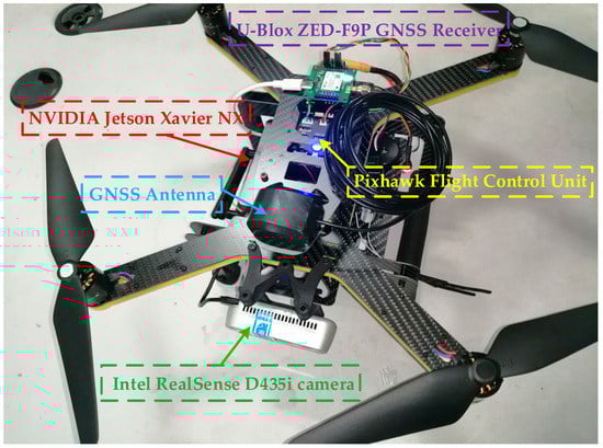
Figure 1. The self-developed agile drone is equipped with the LDMF navigation system.

• The LDMF system leverages the Kanade–Lucas [13] algorithm to track multiple visual feature descriptors [14] in each video frame, and the image corner describing and matching between adjacent frames are not required in the corner tracking procedure. Moreover, our system supports multiple types of cameras, such as monocular, binocular, and RGB-D. After NVIDIA CUDA acceleration, the robot pose estimator can achieve camera-rate (30Hz) performance on a single-board computer.
• The LDMF navigation system can not only quickly provide the drone pose and velocity to the trajectory planner, but also synchronously generate the environment map for automatic obstacle avoidance. Furthermore, the additional marginalization strategy discharged the computation complexity of the LDMF system.
• By entirely using the GNSS raw measurements, the intrinsic drift from the vision-IMU odometry will be dumped, and the yaw angle residual between the odometry frame and the world frame will be updated without any offline calibration. The drone state estimator is able to execute rapidly in unpredictable scenarios and achieves local smooth and global drift-free characteristics without visual closed-loop detection.

2. Related Work

Academic researches on drone pose estimation algorithms are extensive. Noticeable approaches include PTAM [15], ORB-SLAM [8,16,17], RGBD-SLAM [18], LSD-SLAM [19], and OpenVINS [20]. In this section, however, we omit the overview of unfeasible approaches for drone state estimation and pay extra attention to the small-size and economical sensors, such as cameras, inertial measurement units, and GNSS receivers, to achieve autonomous and safe navigation in unknown environments.

2.1. Visual Odometry

Visual odometry (VO) has solved autonomous drone navigation using vision sensors. A single monocular camera is the most straightforward vision sensor in the visual odometry method. Different from other sensors, cameras are passive, accessible, and power efficient. Consequently, vision-based methods have been widely used in robot state estimation. Visual odometry was initially solved by extended Kalman filter (EKF) based methods [21], i.e., every input image is filtered to calculate the camera pose and the corner locations jointly. Filter-based methods have some shortcomings that eventuate accumulative errors and the additional calculation with little new information. Correspondingly, keyframe-based strategies [16,17] calculate the camera pose using laconic image frames allowing to implementation of more complicated but accurate bundle adjustment optimizations. Bundle adjustment is an algorithm based on the least square principle, which is commonly used in the field of photogrammetry. Bundle adjustment calculates the camera pose and the three-dimensional map points as unknown parameters and uses the coordinates of the map points as observation data to obtain the optimal camera pose. Some literature [22] has confirmed that keyframe-based approaches are more precise than counterparts with the same calculation complexity.

In probability theory, probabilistic graph optimization is a widely used model in Bayesian reasoning. Factorizing a global function with multiple variables can obtain the product of several local functions. Inspired by this principle, the residuals can be easily constructed. The back-end modules of keyframe-based SLAM are often constructed by probabilistic graph optimization. PTAM [15] was the first keyframe-based SLAM system, which introduced the trick of splitting feature tracking and map building in parallel threads and has been successfully applied to solve real-time augmented reality problems. The feature matching process of PTAM [15] extracts FAST features matched from each image frame, which causes the corners to only be valid for feature tracking but not for loop detection. Inspired by the above strategies, the ORB-SLAM series [8,16,17], a graph optimization-based visual simultaneous localization and mapping (SLAM) system, makes full use of the oriented fast and rotated brief (ORB) features to construct a covisibility graph to limit the computational cost. The experimental results show that ORB-SLAM [8] can execute in indoor and outdoor environments and deploy on ground robots, agile drones and hand-held motions. The localization errors of ORB-SLAM [8] are generally below one centimeter in small indoor scenes and a few meters in large outdoor scenes.

Direct methods do not extract corners from image frames but directly collect the pixel intensities over the input frames and calculate the camera pose by minimizing a photometric error. LSD-SLAM [19] could map large-scale semi-dense scenarios using direct methods instead of bundle adjustment over image features. LSD-SLAM [19] is able to operate in real-time as the low computational complexity of the system brings about more potential applications for 3D dense map construction than feature-based visual odometry. Regrettably, their pose estimation accuracy is critically lower than the feature-based methods. A hybrid between feature and direct-based strategies is the semi-direct visual SLAM. SVO [23] tracks FAST features with a nonzero intensity gradient from image to image. In the meantime, it optimizes robot pose and environmental map using reprojection error. Benefiting from the system without requiring to feature matching in every input image, SVO [23] was able to operate at high speed in embedded computers equipped with a small drone. Due to the lack of global consistency, however, localization errors will accumulate with the camera translating.

2.2. Multisensor Fusion State Estimation

In the field of robot autonomous navigation, multifarious sensor fusion has become increasingly dominant in recent years because multisensor fusion can steadily provide a robot pose by exploiting the complementary characteristics of each sensor. The simplest method to amalgamate raw data derived from various sensors is loosely coupled data fusion [24], where the measurements from each sensor are solved respectively, and the obtained results are fused. During this period, each sensor is treated as an independent module. The specific sensor fusion process is usually executed through the extended Kalman filter (EKF), where one sensor is used to transmit system states, and other sensors are used to update results. Unlike loosely coupled sensor fusion, the tightly coupled sensor fusion strategies leverage either filter-based or graph optimization-based methods, where all input data are optimized together from the raw measurement level.

The multi-state constraint Kalman filter (MSCKF) [21], an emblematic filter-based visual-inertial odometry, holds several prior camera trajectories in the robot pose vector and exploits the geometric constraints between multiple camera views that observed a particular image feature to update the robot states efficiently. Compared with the filter-based multisensor fusion methods, the nonlinear optimization-based methods hold and estimate all previous system states to obtain the optimal robot poses, which can achieve better localization accuracy at the expense of calculation amount. Unfortunately, owing to excessive computational complexity during the iterative solution, few nonlinear optimization-based approaches can achieve real-time performance on micro robots, such as an agile drone. To make the system quick enough, nonlinear optimization-based approaches [25,26] usually calculate the robot state over a bounded sliding window that is implemented by marginalizing out old system states and sensor measurements. Open keyframe-based visual-inertial SLAM (OKVIS) [27] is a nonlinear optimization-based multisensor fusion system that optimizes robot pose in a bounded container. The residual term is respectively formulated with a weighting of photo geometry reprojection factor and inertial measurement factor. VINS-Fusion [28] and Kimera [29] also estimate robot poses in a bounded container with pose graph optimization, but they increase a particular module to recover odometry from tracking failures. It should be noted that since the local-aware sensors (e.g., camera, IMU, and LiDAR) only impose local relative constraints among robot states, accumulation error is an inevitable crux in a local-aware sensor-based navigation system, especially over long-range movement.

Compared with local-aware sensors, global-aware sensors (e.g., GNSS receivers, magnetometers, and barometers) are dominant for long-distance navigation within large-scale environments. Since local-aware sensors achieve impressive performance in small-scale environments and global-aware sensors have no accumulated error, it is an ingenious tactic to fuse both of them together to achieve locally accurate and globally drift-free drone autonomous navigation. As GNSS provides a globally aware solution in the earth-centered frame, fusing GNSS messages is an artful way to alleviate cumulative drift. In terms of a loosely coupled manner, Lynen et al. [30] fuse visual-inertial odometry with GNSS information for robot pose estimation. Shen et al. [31] utilize an unscented EKF method to fuse different kinds of sensors to produce an accurate and consecutive robot pose. VINS-Fusion [28] combines the position results from different sensors under the optimization-based framework to achieve low-drift robot trajectories. GVINS [10] extensively surveys the system performance in several wide ranges of scenarios, where many existing dynamic targets and less than four navigation satellites are captured. All works mentioned above rely on consecutive source information to solve system states, which again limits the practical application of the multisensor fusion state estimation.

3. System Overview

The drone pose includes the current position and orientation in the world coordinate system. In our software development, the drone pose is represented by a 3D space point and a quaternion. We define (⁎)^r as the robot coordinate system. (⁎)^o is the odometry frame, where the direction of gravity is aligned with the Z axis. World coordinate system (⁎)^w is a semi-global frame, where the X and Y axes respectively direct to the east and north direction, and the Z axis is also gravity aligned. The earth-centered, earth-fixed (ECEF) frame (⁎)^e and the earth-centered inertial (ECI) frame (⁎)^e are the global coordinate system that is fixed concerning the center of the earth. The complete frame transformation relationship is diagrammed in Figure 2, and the coordinate transformation tree is illustrated in Figure 3. The difference between the ECEF and the ECI frame is that the latter’s coordinate axis does not change with the earth’s rotation.

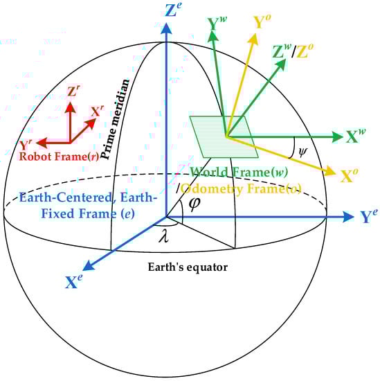
Figure 2. Diagram above shows the complete frame transformation relationship.

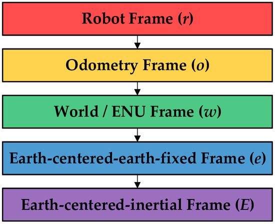
Figure 3. The coordinate transformation tree in our proposed navigation system.

The structure of the LDMF system overview is diagrammed in Figure 4. The sensor raw data from the drone companion computer are preprocessed, including visual feature extraction and tracking, IMU measurements pre-integration, and GNSS raw signal filtering. Vision-IMU-GNSS information is jointly initialized to obtain all the initial values of the drone pose estimator. During navigation system initialization, the IMU original measurements are pre-integrated [32,33] to initialize the vision-IMU tightly coupled drone odometry. Then, an imperfect drone position in the world coordinate frame is solved by the single point positioning (SPP) algorithm. Finally, probability factor graph optimization modifies the drone pose in the global coordinate system.

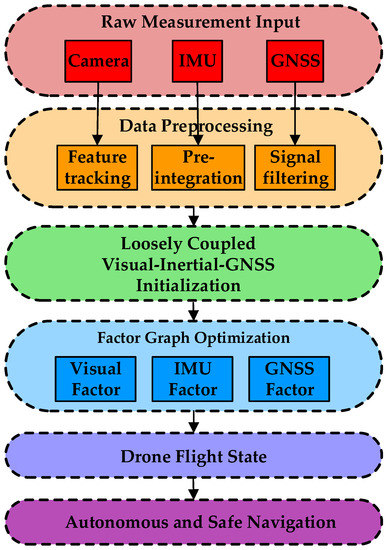
Figure 4. The flowsheet of the LDMF autonomous navigation system.

When the drone state estimator is initialized, constraints from all sensor measurements are tightly coupled to calculate drone states within a small sliding window. In order to maintain the real-time performance of the proposed LDMF system, the additional marginalization scheme [29] is also effectuated after each optimization.

4. Multisensor Fusion Strategy

4.1. Formulation

In this section, multisensor fusion is formulated as a probabilistic factor graph optimization procedure, which constrains the drone states in flight. The factors in the probabilistic graph are composed of visual factor, inertia factor and navigation satellite factor. All factors in the factor graph will be formulated in detail through this section. The whole system states inside the circumscribed container can be summarized as follows:

$$\left\{\begin{array}{l}\chi ={\left[x_0,x_1, \dots , x_n,{\lambda }_1,{\lambda }_2,\dots ,{\lambda }_m,\psi \right]}^T\hfill \\ xk={\left[o_{r_{tk}}^w,v_{r_{tk}}^w,p_{r_{tk}}^w,b_{{\omega }_{tk}},b_{a_{tk}},\delta t,\delta t^{\prime }\right]}^T, k\in \left[0,n\right]\hfill \end{array}\right.$$

(1)

where x_k is the drone flight state at the time tk that the kth video frame is captured. It contains airframe orientation $o_{r_{tk}}^w$, velocity $v_{r_{tk}}^w$, position $p_{r_{tk}}^w$, gyroscope bias $b_{{\omega }_{tk}}$ and acceleration bias $b_{a_{tk}}$ of the drone in the odometry frame. $\delta t$ and $\delta t^{\prime }$ correspond to the clock biases and bias drifting rate of the GNSS receiver, respectively. n is the sliding window size, and m is the total number of visual features in the sliding window. ${\lambda }_l$ is the inverse depth of the lth visual feature. $\psi$ is the yaw bias between the odometry and the world frame.

4.2. Visual Constraint

The visual factor constraint in the probabilistic graph is constructed from a sequence of sparse corner points. For each input video frame, when the number of feature points is less than 100, new corner points are extracted to maintain a sufficient number of tracking features. Assume the homogeneous coordinates of the image feature point l in the world coordinate frame are:

$${\tilde{p}}_l^w={\left[\raisebox{1ex}{$X_l$}\!\left/ \!\raisebox{-1ex}{$Z_l$}\right., \raisebox{1ex}{$Y_l$}\!\left/ \!\raisebox{-1ex}{$Z_l$}\right., 1\right]}^T$$

(2)

Then the homogeneous coordinates of feature point l in the pixel plane of video frame i can be expressed as:

$${\tilde{\mathcal{P}}}_l^{c_i}={\left[u_l^i, v_l^i, 1\right]}^T$$

(3)

The projection model of the airborne camera can be expressed as follows:

$${\tilde{\mathcal{P}}}_l^{c_i}=𝒦T_r^c{T}_w^{r_i}{\tilde{p}}_l^w+n_c$$

(4)

where T is the transformation matrix, n_c is the camera imaging noise, and $𝒦$ is the camera internal parameter matrix:

$$𝒦=\left[\begin{array}{ccc}{f}_x& 0& c_x\\ 0& f_y& c_y\\ 0& 0& 1\end{array}\right]$$

(5)

The elements of the internal parameter matrix can be obtained by the camera calibration process, and the reprojection model of the feature point l from the video frame i to the video frame j can be formulated as:

$${\widehat{\tilde{\mathcal{P}}}}_l^{c_j}=𝒦T_r^c{T}_w^{r_j}\left[T_{r_i}^w{T}_c^r{𝒦}^{-1}\left(Z_l^{c_i}{\tilde{\mathcal{P}}}_l^{c_i}\right)\right]$$

(6)

with

$$Z_l^{c_i}={\lambda }_l^{c_i}\frac{f_x{f}_y}{\sqrt{f_x{}^2{f}_y{}^2+{\left(u_l^i-c_x\right)}^2{f}_y{}^2+{\left(v_l^i-c_y\right)}^2{f}_x{}^2}}$$

(7)

where ${\lambda }_l^{c_i}$ represents the inverse depth of feature point l relative to the airborne camera c_i.

Then the visual factor constraint can be expressed as the deviation between the actual position ${\tilde{\mathcal{P}}}_l^{c_j}$ and the measurement position ${\widehat{\tilde{\mathcal{P}}}}_l^{c_j}$ of the image feature point l in the video frame j:

$$E_V\left({\widehat{z}}_l^{c_j},{\chi }_V\right)={\tilde{\mathcal{P}}}_l^{c_j}-{\widehat{\tilde{\mathcal{P}}}}_l^{c_j}$$

(8)

where ${\chi }_V$ represents the sub-vector related to visual information from the drone flight state vector $\chi$.

4.3. Inertial Measurements Constraint

The inertial measurements include two parts: gyroscope measurement ${\widehat{\omega }}^{r_t}$ and accelerometer measurement ${\widehat{a}}^{r_t}$. Both are affected by the gyroscope bias b_ω and the acceleration bias b_a, respectively. The raw measurement values of the gyroscope and accelerometer can be constructed by the following formulas:

$$\left\{\begin{array}{l}{\widehat{\omega }}^{r_t}={\omega }^{r_t}+b_{{\omega }^{r_t}}+n_{{\omega }^{r_t}}\hfill \\ {\widehat{a}}^{r_t}=a^{r_t}+b_{a^{r_t}}+n_{a^{r_t}}+R_w^{r_t}{g}^w\hfill \end{array}\right.$$

(9)

where the symbols ${\widehat{\omega }}^{r_t}$ and ${\widehat{a}}^{r_t}$, respectively, represent the measured values of the gyroscope and accelerometer at time t with the current IMU body coordinate system as the reference system. b_ω and b_a are the gyroscope bias and accelerometer bias, respectively. n_ω and n_a are gyroscope noise and accelerometer noise, and g_w is the gravitational acceleration.

Assuming that the time of drone flight in two consecutive video frames is t_k and t_k+1, then the orientation (o), velocity (v), and position (p) of the drone at time t_k+1 in the local world coordinate system can be expressed by the following formula:

$$\left\{\begin{array}{l}{o}^{w_{tk+1}}=o^{w_{tk}}\otimes {\displaystyle {\int }_{t\in [tk,tk+1]}\frac{1}{2}}\Phi ({\widehat{\omega }}^{r_t}-b_{{\omega }^{r_t}}-n_{{\omega }^{r_t}})o_{r_t}^{r_{tk}}dt\hfill \\ v^{w_{tk+1}}=v^{w_{tk}}+{\displaystyle {\int }_{t\in [tk,tk+1]}\left[R_{r_t}^{w_t}({\widehat{a}}^{r_t}-b_{a^{r_t}}-n_{a^{r_t}})-g^{w_t}\right]}dt\hfill \\ p^{w_{tk+1}}=p^{w_{tk}}+(t_{k+1}-t_k)v^{w_{tk}}+{\displaystyle {\iint }_{t\in [tk,tk+1]}\left[R_{r_t}^{w_t}({\widehat{a}}^{r_t}-b_{a^{r_t}}-n_{a^{r_t}})-g^{w_t}\right]}d{t}^2\hfill \end{array}\right.$$

(10)

where

$$\Phi (\omega )=\left[\begin{array}{cc}-{⌊\omega ⌋}_{\times }& \omega \\ -{\omega }^T& 0\end{array}\right],{⌊\omega ⌋}_{\times }=\left[\begin{array}{ccc}0& -{\omega }_z& {\omega }_y\\ {\omega }_z& 0& -{\omega }_x\\ -{\omega }_y& {\omega }_x& 0\end{array}\right]$$

(11)

In the above formula, the symbol $\otimes$ represents quaternion multiplication and symbols $\widehat{\omega }$ and $\widehat{a}$ represent the measured values from the gyroscope and accelerometer.

If the reference coordinate system is converted from the local world coordinate system (w) to the robot fuselage coordinate system (r), the above formula can be rewritten as:

$$\left\{\begin{array}{l}{o}_w^{r_{tk}}\otimes o^{w_{tk+1}}={\alpha }_{r_{tk+1}}^{r_{tk}}\hfill \\ R_w^{r_{tk}}{v}^{w_{tk+1}}=R_w^{r_{tk}}[v^{w_{tk}}-(t_{k+1}-t_k)g^w]+{\beta }_{r_{tk+1}}^{r_{tk}}\hfill \\ R_w^{r_{tk}}{p}^{w_{tk+1}}=R_w^{r_{tk}}[p^{w_{tk}}+(t_{k+1}-t_k)v^{w_{tk}}-\frac{1}{2}{g}^w{(t_{k+1}-t_k)}^2]+{\gamma }_{r_{tk+1}}^{r_{tk}}\hfill \end{array}\right.$$

(12)

where the IMU pre-integration term can be expressed as:

$$\left\{\begin{array}{l}{\alpha }_{r_{tk+1}}^{r_{tk}}={\alpha }_{r_t}^{r_{tk}}{\displaystyle {\int }_{t\in [tk,tk+1]}\frac{1}{2}}\Phi ({\widehat{\omega }}^{r_t}-b_{{\omega }^{r_t}}-n_{{\omega }^{r_t}})dt\hfill \\ {\beta }_{r_{tk+1}}^{r_{tk}}={\displaystyle {\int }_{t\in [tk,tk+1]}{R}_{r_t}^{r_{tk}}}({\widehat{a}}^{r_t}-b_{a^{r_t}}-n_{a^{r_t}})dt\hfill \\ {\gamma }_{r_{tk+1}}^{r_{tk}}={\displaystyle {\iint }_{t\in [tk,tk+1]}{R}_{r_t}^{r_{tk}}}({\widehat{a}}^{r_t}-b_{a^{r_t}}-n_{a^{r_t}})d{t}^2\hfill \end{array}\right.$$

(13)

In tensor calculus, the Jacobian matrix is a matrix formed by arranging the first-order partial derivatives in a certain way. The function of the Jacobian matrix is that it approximates a differentiable equation and the optimal linear approximation of the given input. Therefore, the Jacobian matrix is similar to the derivative of a multivariate function. Then the Jacobian matrix corresponding to the IMU pre-integration term can be expressed as:

$$J_{t+\delta t}^{\alpha }=\left(\delta t{𝒬}_t+I\right)J_t^{\alpha }$$

(14)

where symbol I represents the identity matrix, and

$${𝒬}_t=\left[\begin{array}{lllll}0& I& \hfill 0\hfill & \hfill 0\hfill & \hfill 0\hfill \\ 0& 0& \hfill -R_t^{r_{tk}}{⌊{\widehat{a}}^{r_t}-b_{a^{r_t}}⌋}_{\times }\hfill & \hfill -R_t^{r_{tk}}\hfill & \hfill 0\hfill \\ 0& 0& \hfill -{⌊{\widehat{\omega }}^{r_t}-b_{{\omega }^{r_t}}⌋}_{\times }\hfill & \hfill 0\hfill & \hfill -I\hfill \\ 0& 0& \hfill 0\hfill & \hfill 0\hfill & \hfill 0\hfill \\ 0& 0& \hfill 0\hfill & \hfill 0\hfill & \hfill 0\hfill \end{array}\right]$$

(15)

Then the first-order Jacobian approximation of the IMU pre-integration term can be expressed by the following formula:

$$\left\{\begin{array}{l}{\alpha }_{r_{tk+1}}^{r_{tk}}\approx {\widehat{\alpha }}_{r_{tk+1}}^{r_{tk}}\otimes \left[\begin{array}{c}1\\ \frac{1}{2}{J}_{b\omega }^{\alpha }\Delta b{\omega }_{tk}\end{array}\right]\\ {\beta }_{r_{tk+1}}^{r_{tk}}\approx {\widehat{\beta }}_{r_{tk+1}}^{r_{tk}}+J_{ba}^{\beta }\Delta b{a}_{tk}+J_{b\omega }^{\beta }\Delta b{\omega }_{tk}\\ {\gamma }_{r_{tk+1}}^{r_{tk}}\approx {\widehat{\gamma }}_{r_{tk+1}}^{r_{tk}}+J_{ba}^{\gamma }\Delta b{a}_{tk}+J_{b\omega }^{\gamma }\Delta b{\omega }_{tk}\end{array}\right.$$

(16)

This formula represents a sub-matrix in the Jacobian matrix. When the gyroscope or accelerometer bias changes, the above first-order Jacobian approximation can replace the IMU pre-integration without reintegration.

The gyroscope factor constraint term is constructed as a rotation residual based on the quaternion outer product. Then the complete IMU factor constraint can be constructed as follows:

$$\begin{array}{cc}& E_I\left({\widehat{z}}_{r_{tk+1}}^{r_{tk}},{\chi }_I\right)\hfill \\ & ={\left[{\alpha }_{r_{tk+1}}^{r_{tk}}\otimes {\left({\widehat{\alpha }}_{r_{tk+1}}^{r_{tk}}\right)}^{-1},{\beta }_{r_{tk+1}}^{r_{tk}}-{\widehat{\beta }}_{r_{tk+1}}^{r_{tk}},{\gamma }_{r_{tk+1}}^{r_{tk}}-{\widehat{\gamma }}_{r_{tk+1}}^{r_{tk}},\delta b_{\omega },\delta b_a\right]}^T\hfill \\ & =\left[\begin{array}{c}2{\left[o_w^{r_{tk}}\otimes o^{w_{tk+1}}\otimes {\left({\widehat{\alpha }}_{r_{tk+1}}^{r_{tk}}\right)}^{-1}\right]}_{imag}\\ R_w^{r_{tk}}\left[v^{w_{tk+1}}-v^{w_{tk}}+(t_{k+1}-t_k)g^w\right]-{\widehat{\beta }}_{r_{tk+1}}^{r_{tk}}\\ R_w^{r_{tk}}\left[p^{w_{tk+1}}-p^{w_{tk}}-(t_{k+1}-t_k)v^{w_{tk}}+\frac{1}{2}{g}^w{(t_{k+1}-t_k)}^2\right]-{\widehat{\gamma }}_{r_{tk+1}}^{r_{tk}}\\ b_{{\omega }^{r_{t+1}}}-b_{{\omega }^{r_t}}\\ b_{a^{r_{t+1}}}-b_{a^{r_t}}\end{array}\right]\hfill \end{array}$$

(17)

where ${\chi }_I$ represents the sub-vector related to IMU in the drone flight state vector $\chi$.

4.4. GNSS Constraint

The GNSS factor constraint in the probability factor graph model is composed of three modules, i.e., pseudo-range factor, Doppler frequency shift factor and receiver clock offset factor. The pseudo-range measurement model between the ground receiver and the navigation satellite can be expressed as follows:

$${\widehat{P}}_r^s=‖p_r^E-p_s^E‖+c\left(\delta t_r+\delta t_s+\Delta t_{tro}+\Delta t_{ion}+\Delta t_{mul}\right)+n_{pr}$$

(18)

with

$$\left\{\begin{array}{c}{p}_{r_{tk}}^E=R({\omega }_{\mathrm{earth}}{t}_r^s)p_{r_{tk}}^e\\ p_{s_i}^E=R({\omega }_{\mathrm{earth}}{t}_r^s)p_{s_i}^e\end{array}\right.$$

(19)

Here, $p_r^E$ and $p_s^E$ are the positions of the ground receiver and navigation satellite in the earth-centered inertial coordinate system, respectively. ${\widehat{P}}_r^s$ is the measured value of GNSS pseudo-range, c is the propagation speed of light in vacuum, $\delta t_r$ and $\delta t_s$ are the clock offset of the receiver and satellite, respectively, $\Delta t_{tro}$ and $\Delta t_{ion}$ are the delay of troposphere and ionosphere in the atmosphere, respectively, $\Delta t_{mul}$ is the delay caused by multipath effect, $n_{pr}$ is the noise of pseudo-range signal, and ${\omega }_{\mathrm{earth}}$ is the earth’s rotation speed. $t_r^s$ represents the signal propagation time from the satellite to the receiver.

Then the GNSS pseudo-range factor constraint can be constructed as the residual between the true pseudo-range and the receiver-measured pseudo-range:

$$E_{pr}\left({\widehat{z}}_{r_{tk}}^{s_i},{\chi }_{pr}\right)=‖p_{r_{tk}}^E-p_{s_i}^E‖+c\left(\delta t_{r_{tk}}+\delta t_{s_i}+\Delta t_{tro}+\Delta t_{ion}+\Delta t_{mul}\right)-{\widehat{P}}_{r_{tk}}^{s_i}$$

(20)

where ${\chi }_{pr}$ represents the sub-vector related to the GNSS pseudo-range message in the drone flight state vector $\chi$.

Besides the pseudo-range message, Doppler frequency shift is also an important navigation information in GNSS modulated signal. The Doppler frequency shift measurement between the ground receiver and navigation satellite can be modeled as follows:

$$\delta {\widehat{f}}_r^s=-\frac{1}{\lambda }\left[{\Im }_r^s\left(v_r^E-v_s^E\right)+c\left(\delta t_r{}^{\prime }+\delta t_s{}^{\prime }\right)\right]+n_{dp}$$

(21)

with

$$\left\{\begin{array}{c}{v}_{r_{tk}}^E=R({\omega }_{\mathrm{earth}}{t}_r^s)v_{r_{tk}}^e\\ v_{s_i}^E=R({\omega }_{\mathrm{earth}}{t}_r^s)v_{s_i}^e\end{array}\right.$$

(22)

where $\lambda$ is the carrier wavelength, ${\Im }_r^s$ represents the direction vector between the GNSS receiver and navigation satellite, $v_{r_{tk}}^E$ and $v_{s_i}^E$ represent the relative velocity between the GNSS receiver and navigation satellite, respectively. $\delta t_{r_{tk}}{}^{\prime }$ and $\delta t_{s_i}{}^{\prime }$ are the clock offset drifting rate with the receiver and the satellite, respectively.

Then the GNSS Doppler shift factor constraint can be constructed as the residual between the true carrier Doppler shift and the Doppler shift measurement:

$$E_{dp}\left({\widehat{z}}_{r_{tk}}^{s_i},{\chi }_{dp}\right)=-\frac{1}{\lambda }\left[{\Im }_{r_{tk}}^{s_i}\left(v_{r_{tk}}^E-v_{s_i}^E\right)+c\left(\delta t_{r_{tk}}{}^{\prime }+\delta t_{s_i}{}^{\prime }\right)\right]-\delta {\widehat{f}}_{r_{tk}}^{s_i}$$

(23)

where ${\chi }_{dp}$ represents the sub-vector related to GNSS Doppler frequency shift in the drone flight state vector $\chi$ and $\delta {\widehat{f}}_{r_{tk}}^{s_i}$ is the Doppler frequency shift measurement value.

Now, the GNSS receiver clock offset error from t_k to t_k+1 is constructed as follows:

$$E_{\tau }\left({\widehat{z}}_{k-1}^k,{\chi }_{\tau }\right)=\delta t_{r_{tk}}-\delta t_{r_{tk-1}}-\left(t_k-t_{k-1}\right)\delta t_{r_{tk-1}}{}^{\prime }$$

(24)

By combining the pseudo-range factor $E_{pr}$, the Doppler frequency shift factor $E_{dp}$, and the receiver clock offset factor $E_{\tau }$, the GNSS factor constraint item in the drone state probability factor graph can be formed.

4.5. Tightly Coupled Drone Flight State Estimation

The drone flight pose-solving process is a state estimation problem. The optimal solution is the maximum a posteriori estimation of the drone flight state vector $\chi$. Assuming that the measurement noise conforms to a Gaussian distribution with zero mean, then the solution process of the drone flight state vector $\chi$ can be expressed as:

$$\begin{array}{l}\chi =\underset{\chi }{\arg \mathrm{m}\mathrm{a}\mathrm{x}}P\left(\chi |z\right)\\ \hspace{0.17em}=\underset{\chi }{\arg \min }\left({‖ep-Hp\chi ‖}^2+{\displaystyle \sum _{k=1}^n{‖E\left(z_k,\chi \right)‖}^2}\right)\end{array}$$

(25)

where z is the drone pose linear observation model, H_P matrix means the prior drone pose information obtained by the airborne camera, n is the number of drone flight state vectors in the sliding window, and E(ˑ) implies the sum of all sensor measurement error factors.

Finally, the complete drone pose information can be obtained by solving the drone flight state vector $\chi$ by means of probability factor graph optimization.

5. Experiments

5.1. Benchmark Tests in Public Dataset

The EuRoC datasets [34] are collected from a binocular fisheye camera and synchronized inertial measurement unit carried by an agile drone. The EuRoC datasets [34] contain 11 videotapes, including different lighting conditions and scenarios. We compare the proposed LDMF system with OKVIS [27] and VINS-Fusion [28] in EuRoC datasets. OKVIS is another nonlinear optimization-based visual-inertial pose estimator, and VINS-Fusion [28] is the state-of-the-art sliding window-based tightly coupled agent state estimator.

All methods are compared in an NVIDIA Jetson Xavier NX computer, as shown in Figure 5. The NVIDIA Jetson series devices are slightly different from other onboard computers because it has a GPU module with 384 CUDA cores, which allows the LDMF system to be operated in real-time with CUDA parallel acceleration. The comparison of experimental results on root-mean-square error (RMSE) is shown in Table 1, which is verified by an absolute trajectory error (ATE). Due to the lack of GNSS navigation messages in the EuRoC datasets, the LDMF system will inevitably generate some accumulation error over time, an inherent characteristic of all local sensor-based robot pose estimators. Fortunately, thanks to the local bundle adjustment, the accumulation error of the LDMF system is always within a tolerable range, even if no GNSS messages are received. The experimental results show that, on the NVIDIA Jetson Xavier NX embedded platform, the LDMF system shows exceptional accuracy compared to other state-of-the-art visual-inertial-based robot odometry.

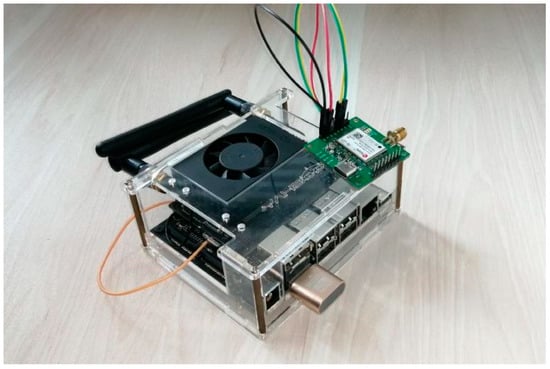
Figure 5. The NVIDIA Jetson Xavier NX embedded computer is exploited in our evaluation.

Table 1. Performance comparison judged by absolute trajectory errors in meters.

Sequence	OKVIS	VINS-Fusion	LDMF
MH01	0.16	0.18	0.17
MH02	0.22	0.12	0.14
MH03	0.24	0.23	0.13
MH04	0.34	0.29	0.23
MH05	0.47	0.25	0.35
V101	0.09	0.12	0.07
V102	0.20	0.13	0.11
V103	0.24	0.07	0.13
V201	0.13	0.09	0.07
V202	0.16	0.14	0.09
V203	0.29	0.23	0.18
Average	0.23	0.17	0.15

5.2. Real-World Position Estimation Experiments

5.2.1. Experimental Preparation

As exhibited in Figure 6, the equipment employed in our real-world position estimation experiments is a multisensor package with a stereo camera, a standard precision IMU and a GNSS receiver. The detailed descriptions of each sensor are shown in Table 2. The Intel RealSense D435i is a stereo camera with the addition of a BMI055 inertial measurement unit. Its field of view (FOV) exceeds 104 degrees, and the image sensor supports a global shutter. We utilize WIT JY901B inertial navigation module to provide raw inertial information. This inertial module has equipped with an MPU-9250 microchip, which can continuously output the raw IMU measurements at a frequency of 200 Hz. The u-blox ZED-F9P is a high-performance GNSS receiver with multi-constellation support, and it integrates real-time kinematics (RTK) technology in a compact encapsulation to acquire centimeter-level accuracy in an open-air scene. ZED-F9P offers support for a range of carrier ambiguity correction modalities allowing each application to improve navigation precision.

Figure 6. The multisensor package is employed in our real-world position estimation experiments. The uncertainty of each sensor is well synchronized via the GNSS receiver’s pulse per second (PPS) signal.

Table 2. The detailed descriptions of each sensor employed in real-world estimation experiments.

Sensor Item	Specification	Unit
Vision
Model Number	Intel D435i
Image Technology	Global Shutter
Resolution	640 × 480	pixel
Field of View	87 × 58	degree
Frame Rate	30	FPS
Size	90 × 25 × 25	mm
Inertia
Microchip	MPU-9250
Gyroscope Resolution	0.061	º/s
Gyroscope Noise	0.028~0.07	º/s
Gyroscope Zero Drift	±0.5	º/s
Accelerometer Resolution	0.0005	g
Accelerometer Noise	0.75~1	mg
Accelerometer Zero Drift	±20~40	mg
Frequency	200	Hz
GNSS
Antenna	BenTian-3070
Gain	35 ± 2	dB
Receiver	u-blox ZED-F9P
Error Range	1.5	m
Frequency	10	Hz

In order to provide a reliable ground truth for the experiments, as displayed in Figure 7, another u-blox ZED-F9P is arranged near the mobile receiver as a base station to feed it with a continuous RTCM stream. In other words, a total of two u-blox ZED-F9P modules are required in the real-world position estimation experiments, one as the ambulatory rover and the other as the stationary base station, to correct the position of the mobile rover. RTK base station forwards the RTCM stream to the GNSS receiver’s serial port through transmission control protocol (TCP). It is worth noting that the GNSS information after RTCM correction is only used to evaluate the performance of the fusion algorithms in this paper and will not participate in any practical multisensor fusion process. To eliminate the uncertainty from different sensors, the time of each sensor is subject to the robot operating system (ROS) time, and the ROS time is aligned with the universal time coordinated (UTC) via the pulse per second (PPS) signal of the GNSS receiver.

Figure 7. An RTK base station is used to provide a continuous RTCM stream for the GNSS receiver.

5.2.2. Pure Rotation Test on a Soccer Field

Due to the inherent imperfections of local sensors, the motion trajectory of visual-inertial odometry will inevitably drift over time. In general, the common visual-inertial pose estimator can achieve good performance when the robot moves in translation, but it does not perform well when the robot moves in pure rotation. In order to assess the performance of the LDMF system under the condition of pure rotation, we carried out experiments on a campus soccer field, where there are no buildings or big trees around this place so that the GNSS receiver can continuously lock the navigation satellite.

We put the RTK base station over the center of the soccer field. When the RTK status changes from “float” to “fixed”, we move along the soccer field sideline, midline and goal line in a straight line with the sensor equipment described in the Section 5.2.1. When encountering a corner, we rotate 90 degrees and continue to move along the marker line until we pass all the marker lines on the soccer field. The entire running situation is shown in Figure 8. The red points in Figure 8b,c are the Shi-Tomasi sparse feature points that have successfully completed KLT optical flow tracking, and the blue points are the Shi-Tomasi feature points, but no matching is found. In this experiment, the overall trajectory was 1km, and it took about 14 min to complete the whole journey. During this test the vast majority of navigation satellites are well captured, and the RTK mode keeps fixed throughout the whole experiment.

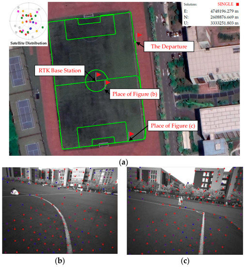
Figure 8. The travel situation of the pure rotation test. (a) The global journey trajectory is drawn on Google Earth; (b) The visual feature state when moving to the central ring on the soccer field; and (c) The visual feature state when moving to the south goal line.

The proposed LDMF system is compared with RTKLIB [35], VINS-Fusion [28] and GVINS [10]. All assessments in this section are conducted on an NVIDIA Jetson Xavier NX embedded device as before. Table 3 shows the experimental results between LDMF and the other two methods, which are verified by an absolute trajectory error (ATE). There are four evaluation criteria in this test: namely, root mean square error (RMSE), median error, mean error and standard deviation. Figure 9 shows the superiorities of LDMF over other methods more intuitively than Table 3. The LDMF is superior to other methods in all performance criteria. Figure 10 shows the ATE of RTKLIB [35], VINS-Fusion [28], GVINS [10] and our system with respect to the running time. The positioning results from RTKLIB [35], VINS-Fusion [28], GVINS [10] and our system are compared directly against the RTK ground truth. As can be seen from Figure 10, the tightly coupled LDMF system outperforms other methods in the long distance. It benefits from the tight fusion of the global sensor, the cumulative error is limited to a tolerable range, and there is no drift over time. It is noteworthy that the LDMF system has an influential error at the initial stage, which is caused by the asynchronous initialization in the sensor fusion process. The system first initializes the vision module, then integrates with the inertial module, and finally feeds into the navigation satellite information. The positioning error decreases gradually until the system is completely initialized.

Table 3. Performance comparison judged by absolute trajectory errors in soccer field sequence.

Index	RTKLIB	VINS-Fusion	GVINS	LDMF
RMSE	13.11	2.90	1.77	1.39
Median	11.02	2.46	1.27	1.16
Mean Error	11.73	2.59	1.46	1.24
Standard Deviation	5.86	1.32	1.31	0.63
CPU Usage	55%	395%	275%	190%

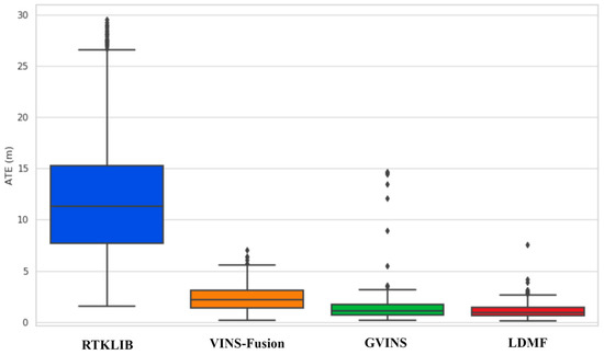
Figure 9. The comparison of absolute trajectory errors between different methods.

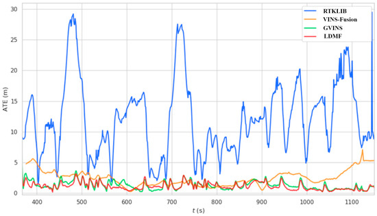
Figure 10. The system consistency on absolute trajectory error as time goes on in the soccer field sequence.

5.2.3. Dynamic Interference Test on an Overpass

In addition to continuous rotary motion, another challenging scenario is the dynamic target interference scene. Next, we will conduct a robustness test for dynamic interference and low illumination by crossing an overpass. The test started at dusk, and it was completely dark by the end of the experiment. During the experiment, a large number of pedestrians passed the stereo camera, which caused considerable dynamic interference to the visual state estimation, and the trees on both sides of the road also increased the GNSS signal noise, which poses a great challenge to the robot navigation system based on a single sensor. Furthermore, the motion trajectory is an arbitrary exploration path where no intersection exists between routes, so a visual closed-loop cannot be formed. Hence drifting is unavoidable for any local-aware sensor-based odometry. We set the starting point as the athletic arena and the destination as the aeronautics park. When the RTK status changed from “3D float” to “fixed”, we began to move northward and boarded the overpass along the sidewalk. Then move along the sky bridge from east to west until crossing the whole bridge. The complete running track is shown in Figure 11. In this robustness test, the overall trajectory was 703 m, and it took 8.5 min to complete the whole journey. Although the navigation satellite locking received some influence due to the shelter of big trees, the RTK state remained fixed throughout the experiment.

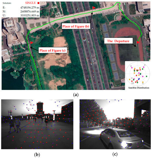
Figure 11. The travel circumstance of the dynamic interference and low illumination test. (a) The global journey trajectory of the large-scale environment is drawn on Google Earth; (b) The visual feature state when the D435i camera on the overpass faces the westward academic building; and (c) The visual feature state when a car coincidentally passes in front of the camera.

We compare the proposed LDMF system with RTKLIB [35], VINS-Fusion [28], and GVINS [10] in this dynamic interference and low illumination experiment. Table 4 shows the experimental results between the LDMF system and the other two methods, and the LDMF is superior to other methods in all performance criteria. A more intuitive comparison is shown in Figure 12, which schematically represents a significant advantage of the proposed LDMF system compared to other state-of-the-art state estimators. Figure 13 shows the ATE of RTKLIB [35], VINS-Fusion [28], GVINS [10] and our system concerning the running time. The positioning results from RTKLIB [35], VINS-Fusion [28], GVINS [10] and our system are compared directly against the RTK ground truth. From Figure 13, we can see that the LDMF system maintains a lower localization error than other methods most of the time. Loosely coupled localization algorithms are seriously interfered with by dynamic interference and illumination variation, even though they do not drift or diverge at all. In benefiting from the tight fusion of the global sensor, the localization error is limited to a reasonable extent in the case of serious external interference.

Table 4. Performance comparison judged by absolute trajectory errors in overpass sequence.

Index	RTKLIB	VINS-Fusion	GVINS	LDMF
RMSE	8.42	2.59	1.87	1.19
Median	6.77	1.83	1.33	0.79
Mean Error	7.54	2.23	1.61	0.95
Standard Deviation	3.73	1.32	1.58	0.73
CPU Usage	55%	385%	270%	190%

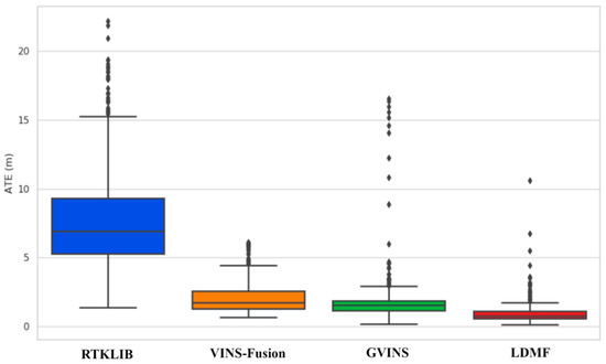
Figure 12. The comparison on absolute trajectory errors between different methods.

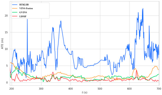
Figure 13. The system consistency on absolute trajectory error as time goes on in the overbridge sequence.

5.3. Autonomous and Safe Navigation with an Agile Drone

We carried out the virtual experiment for drone autonomous and safe navigation in the Gazebo simulator, as shown in Figure 14. After taking off, the aerial robot leverages a virtual plug-in camera, accelerometer, gyroscope and GNSS raw signal to obtain the relative relationship between the robot frame and the world coordinate. Meanwhile, a 3D environmental map calculated by a virtual plug-in camera is structured to further captured the transformation matrix between the aerial robot and the neighboring obstruction. When the flight destination is entered manually, the trajectory planner generates a path for the aerial robot motion and sends the desired speed to the flight controller, then gradually approaches the destination and keeps a fixed distance from the neighboring obstruction.

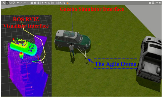
Figure 14. The agile drone autonomous navigation test is carried out in the Gazebo simulator.

In order to verify the robustness and practicability of the proposed multisensor fusion strategies, we conduct both simulation and real-world physical verification, as shown in Figure 1. The inertial measurement unit utilized in our real-world examination is an IMU built into the Pixhawk 2.4.8 flight control unit. In the meantime, an Intel RealSense D435i camera is used to capture environmental maps. In addition, the U-Blox ZED-F9P is employed as a GNSS receiver. The real-world experiment was conducted on a campus tennis court, where the sky is open, and most of the navigation satellites are well-tracked. The terrain crossed by the aerial robot is an arbitrary artificial obstruction, as shown in Figure 15. During the flight, the aerial robot will change its route when approaching an obstacle and always keep a reasonable distance from the neighboring obstruction.

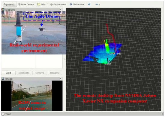
Figure 15. The real-world drone autonomous navigation experiment was conducted on a campus tennis court.

6. Conclusions and Future Work

In this paper, we proposed LDMF: a lightweight and drift-free vision-IMU-GNSS tightly coupled multisensor fusion strategy for drone autonomous and safe navigation, which combines visual, inertial and GNSS raw measurements to estimate drone state between consecutive image frames. In the nonlinear optimization phase, vision-IMU-GNSS raw messages were formulated by the probabilistic factor graph in a narrow sliding window. The LDMF system can achieve real-time drone pose estimation with CUDA acceleration on an embedded airborne computer. The proposed drone navigation system is evaluated using both simulated and real-world experiments, demonstrating noticeable superiorities over state-of-the-art methods.

Although the LDMF system has already reached the maturity for drone autonomous and safe navigation, we still see multiple potential improvements for future work. The magnetic field and atmospheric pressure will not be affected by urban canyons or multipath effects and have been widely used in the field of drone navigation. We plan to design a new fusion strategy for magnetometer and barometer sensors in future work to further provide the performance of the drone navigation system. Furthermore, how to quickly and accurately generate the semantic map around the drone is additional research we will carry out in the future.

References

- Gupta, A.; Fernando, X. Simultaneous Localization and Mapping (SLAM) and Data Fusion in Unmanned Aerial Vehicles: Recent Advances and Challenges. Drones 2022, 6, 85. [Google Scholar] [CrossRef]
- Chen, J.; Li, S.; Liu, D.; Li, X. AiRobSim: Simulating a Multisensor Aerial Robot for Urban Search and Rescue Operation and Training. Sensors 2020, 20, 5223. [Google Scholar] [CrossRef] [PubMed]
- Tabib, W.; Goel, K.; Yao, J.; Boirum, C.; Michael, N. Autonomous Cave Surveying with an Aerial Robot. IEEE Trans. Robot. 2021, 9, 1016–1032. [Google Scholar] [CrossRef]
- Zhou, X.; Wen, X.; Wang, Z.; Gao, Y.; Li, H.; Wang, Q.; Yang, T.; Lu, H.; Cao, Y.; Xu, C.; et al. Swarm of micro flying robots in the wild. Sci. Robot. 2022, 7, eabm5954. [Google Scholar] [CrossRef] [PubMed]
- Paul, M.K.; Roumeliotis, S.I. Alternating-Stereo VINS: Observability Analysis and Performance Evaluation. In Proceedings of the IEEE Conference on Computer Vision and Pattern Recognition (CVPR), Salt Lake City, UT, USA, 18–22 June 2018; pp. 4729–4737. [Google Scholar]
- Qin, T.; Li, P.; Shen, S. VINS-Mono: A robust and versatile monocular visual-inertial state estimator. IEEE Trans. Robot. 2018, 34, 1004–1020. [Google Scholar] [CrossRef]
- Tian, Y.; Chang, Y.; Herrera Arias, F.; Nieto-Granda, C.; How, J.; Carlone, L. Kimera-Multi: Robust, Distributed, Dense Metric-Semantic SLAM for Multi-Robot Systems. IEEE Trans. Robot. 2022, 38, 2022–2038. [Google Scholar] [CrossRef]
- Campos, C.; Elvira, R.; Rodríguez, J.J.G.; Montiel, J.M.M.; Tardós, J.D. ORB-SLAM3: An Accurate Open-Source Library for Visual, Visual–Inertial, and Multimap SLAM. IEEE Trans. Robot. 2021, 37, 1874–1890. [Google Scholar] [CrossRef]
- Li, T.; Zhang, H.; Gao, Z.; Niu, X.; El-sheimy, N. Tight Fusion of a Monocular Camera, MEMS-IMU, and Single-Frequency Multi-GNSS RTK for Precise Navigation in GNSS-Challenged Environments. Remote Sens. 2019, 11, 610. [Google Scholar] [CrossRef]
- Cao, S.; Lu, X.; Shen, S. GVINS: Tightly Coupled GNSS–Visual–Inertial Fusion for Smooth and Consistent State Estimation. IEEE Trans. Robot. 2022, 38, 2004–2021. [Google Scholar] [CrossRef]
- Zhang, C.; Yang, Z.; Fang, Q.; Xu, C.; Xu, H.; Xu, X.; Zhang, J. FRL-SLAM: A Fast, Robust and Lightweight SLAM System for Quadruped Robot Navigation. In Proceedings of the IEEE International Conference on Robotics and Biomimetics (ROBIO), Sanya, China, 27–31 December 2021; pp. 1165–1170. [Google Scholar] [CrossRef]
- Zhang, C.; Yang, Z.; Liao, L.; You, Y.; Sui, Y.; Zhu, T. RPEOD: A Real-Time Pose Estimation and Object Detection System for Aerial Robot Target Tracking. Machines 2022, 10, 181. [Google Scholar] [CrossRef]
- Lucas, B.; Kanade, T. An iterative image registration technique with an application to stereo vision. In Proceedings of the 7th International Joint Conference on Artificial Intelligence, Vancouver, BC, Canada, 24–28 August 1981; pp. 24–28. [Google Scholar]
- Shi, J.; Tomasi. Good features to track. In Proceedings of the IEEE Conference on Computer Vision and Pattern Recognition (CVPR), Seattle, WA, USA, 21–23 June 1994. [Google Scholar]
- Klein, G.; Murray, D. Parallel Tracking and Mapping for Small AR Workspaces. In Proceedings of the IEEE and ACM International Symposium on Mixed and Augmented Reality, Nara, Japan, 13–16 November 2007; pp. 225–234. [Google Scholar]
- Mur-Artal, R.; Montiel, J.M.M.; Tardós, J.D. ORB-SLAM: A Versatile and Accurate Monocular SLAM System. IEEE Trans. Robot. 2015, 31, 1147–1163. [Google Scholar] [CrossRef]
- Mur-Artal, R.; Tardós, J.D. ORB-SLAM2: An Open-Source SLAM System for Monocular, Stereo, and RGB-D Cameras. IEEE Trans. Robot. 2017, 33, 1255–1262. [Google Scholar] [CrossRef]
- Endres, F.; Hess, J.; Sturm, J.; Cremers, D.; Burgard, W. 3-D Mapping With an RGB-D Camera. IEEE Trans. Robot. 2014, 30, 177–187. [Google Scholar] [CrossRef]
- Engel, J.; Schöps, T.; Cremers, D. LSD-SLAM: Large-Scale Direct Monocular SLAM. In Proceedings of the The European Conference on Computer Vision (ECCV), Zurich, Switzerland, 6–12 September 2014; pp. 834–849. [Google Scholar] [CrossRef]
- Geneva, P.; Eckenhoff, K.; Lee, W.; Yang, Y.; Huang, G. OpenVINS: A Research Platform for Visual-Inertial Estimation. In Proceedings of the 2020 IEEE International Conference on Robotics and Automation (ICRA), Paris, France, 31 May–31 August 2020; pp. 4666–4672. [Google Scholar] [CrossRef]
- Mourikis, A.; Roumeliotis, S. A multi-state constraint Kalman filter for vision-aided inertial navigation. In Proceedings of the IEEE International Conference on Robotics and Automation, Rome, Italy, 10–14 April 2007; pp. 3565–3572. [Google Scholar]
- Cadena, C.; Carlone, L.; Carrillo, H.; Latif, Y.; Scaramuzza, D.; Neira, J.; Reid, I.; Leonard, J.J. Past, Present, and Future of Simultaneous Localization and Mapping: Toward the Robust-Perception Age. IEEE Trans. Robot. 2016, 32, 1309–1332. [Google Scholar] [CrossRef]
- Forster, C.; Pizzoli, M.; Scaramuzza, D. SVO: Fast semi-direct monocular visual odometry. In Proceedings of the IEEE International Conference on Robotics and Automation (ICRA), Hong Kong, China, 31 May–7 June 2014. [Google Scholar] [CrossRef]
- Weiss, S.; Achtelik, M.; Lynen, S.; Chli, M.; Siegwart, R. Real-time onboard visual-inertial state estimation and self-calibration of MAVs in unknown environments. In Proceedings of the IEEE International Conference on Robotics and Automation (ICRA), Saint Paul, MN, USA, 14–18 May 2012; pp. 957–964. [Google Scholar] [CrossRef]
- Wang, Y.; Kuang, J.; Li, Y.; Niu, X. Magnetic Field-Enhanced Learning-Based Inertial Odometry for Indoor Pedestrian. IEEE Trans. Instrum. Meas. 2022, 71, 2512613. [Google Scholar] [CrossRef]
- Zhou, B.; Pan, J.; Gao, F.; Shen, S. RAPTOR: Robust and Perception-Aware Trajectory Replanning for Quadrotor Fast Flight. IEEE Trans. Robot. 2021, 37, 1992–2009. [Google Scholar] [CrossRef]
- Leutenegger, S.; Lynen, S.; Bosse, M.; Siegwart, R.; Furgale, P. Keyframe-based visual–inertial odometry using nonlinear optimization. Int. J. Robot. Res. 2015, 34, 314–334. [Google Scholar] [CrossRef]
- Qin, T.; Cao, S.; Pan, J.; Shen, S. A General Optimization-based Framework for Global Pose Estimation with Multiple Sensors. arXiv 2019, arXiv:1901.03642. [Google Scholar]
- Rosinol, A.; Abate, M.; Chang, Y.; Carlone, L. Kimera: An Open-Source Library for Real-Time Metric-Semantic Localization and Mapping. In Proceedings of the IEEE International Conference on Robotics and Automation (ICRA), Paris, France, 31 May–31 August 2020; pp. 1689–1696. [Google Scholar]
- Lynen, S.; Achtelik, M.; Weiss, S.; Chli, M.; Siegwart, R. A robustand modular multi-sensor fusion approach applied to MAV navigation. In Proceedings of the IEEE/RSJ International Conference on Intelligent Robots and Systems, Tokyo, Japan, 3–7 November 2013; pp. 3923–3929. [Google Scholar]
- Shen, S.; Mulgaonkar, Y.; Michael, N.; Kumar, V. Multi-sensor fusion for robust autonomous flight in indoor and outdoor environments with a rotorcraft MAV. In Proceedings of the IEEE International Conference on Robotics and Automation, Hong Kong, China, 31 May–7 June 2014; pp. 4974–4981. [Google Scholar]
- Qin, T.; Li, P.; Shen, S. Relocalization, Global Optimization and Map Merging for Monocular Visual-Inertial SLAM. In Proceedings of the IEEE International Conference on Robotics and Automation (ICRA), Brisbane, Australia, 21–25 May 2018; pp. 1197–1204. [Google Scholar] [CrossRef]
- Qin, T.; Shen, S. Robust initialization of monocular visual-inertial estimation on aerial robots. In Proceedings of the IEEE/RSJ International Conference on Intelligent Robots and Systems (IROS), Vancouver, BC, Canada, 24–28 September 2017; pp. 4225–4232. [Google Scholar] [CrossRef]
- Burri, M.; Nikolic, J.; Gohl, P.; Schneider, T.; Rehder, J. The EuRoC micro aerial vehicle datasets. Int. J. Robot. Res. 2016, 35, 1157–1163. [Google Scholar] [CrossRef]
- Takasu, T.; Yasuda, A. Development of the low-cost RTK-GPS receiver with an open source program package RTKLIB. In Proceedings of the International Symposium on GPS/GNSS, Jeju, Republic of Korea, 4–6 November 2009; Volume 1, pp. 1–6. [Google Scholar]
Disclaimer/Publisher’s Note: The statements, opinions and data contained in all publications are solely those of the individual author(s) and contributor(s) and not of MDPI and/or the editor(s). MDPI and/or the editor(s) disclaim responsibility for any injury to people or property resulting from any ideas, methods, instructions or products referred to in the content. |
© 2023 by the authors. Licensee MDPI, Basel, Switzerland. This article is an open access article distributed under the terms and conditions of the Creative Commons Attribution (CC BY) license (https://creativecommons.org/licenses/by/4.0/).