Robotic Herding of Farm Animals Using a Network of Barking Aerial Drones

Abstract

This paper proposes a novel robotic animal herding system based on a network of autonomous barking drones. The objective of such a system is to replace traditional herding methods (e.g., dogs) so that a large number (e.g., thousands) of farm animals such as sheep can be quickly collected from a sparse status and then driven to a designated location (e.g., a sheepfold). In this paper, we particularly focus on the motion control of the barking drones. To this end, a computationally efficient sliding mode based control algorithm is developed, which navigates the drones to track the moving boundary of the animals’ footprint and enables the drones to avoid collisions with others. Extensive computer simulations, where the dynamics of the animals follow Reynolds’ rules, show the effectiveness of the proposed approach.

1. Introduction

Robot farming plays a critical role in preventing the food crisis caused by future population growth [1]. The past decades have seen the rapid development of robotic crop farming, such as automated crop monitoring, harvesting, weed control, and so forth [2,3]. Deploying robotic automation to improve crop production yields has actually become very popular among farmers. In contrast, research and implementations of robotic livestock farming have been mostly restricted in the fields of virtual fencing [4], animal monitoring and pasture surveying [5,6]. Such applications can improve livestock production yields to some extent. But animal herding as the vital step of livestock farming has long been the least automated. Sheepdogs that have been used for centuries are still the dominant tools of animal herding around the world, and the research on robotic animal herding is still in its infancy. Two main obstacles of robotic animal herding systems are: (1) lack of practical robot-to-animal interactions and the suitable robotic herding platform; and (2) lack of efficient robotic herding algorithm for abundant animals.

The applications of robots to the actual act of animal herding started from the Robot Sheepdog Project in the 1990s [7,8]. These groundbreaking studies achieved gathering a flock of ducks and manoeuvring them to a specified goal position by wheeled robots. The last three decades have only seen a handful of studies on robotic herding with real animals. Recent implementations of robotic animal herding mainly employ ground robots that drive animals through bright colours [9] or collisions [10,11,12]. Reference [9] shows that the robot initially repulsed the sheep at a distance of 60 m; however, after only two further trials, the repulsion distance drops to 10 m. Besides, such ground legged or wheeled robots might not be agile enough to deal with various terrains during herding. Furthermore, the employed Rover robot in [10], Spot robot in [11] and Swagbot in [12] all cost hundreds of thousands US dollars each and are still in the prototype stages. High prices limit their popularity. Interestingly, the real sheepdogs are also expensive because of their years-long training period. A fully trained sheepdog can cost tens of thousands of US dollars [13]. The most crucial drawback of sheepdogs is that they cannot get rid of biological limitations, that is, ageing and illness.

Besides the platforms, efficient algorithms are also critical to the study of robotic animal herding. Despite the stagnant progress of the herding platforms, research of the related algorithms has experienced considerable development. The prime cause of this contradiction is the recent rapid development of the study on swarm robotics and swarm intelligence [14]. Bio-inspired swarming-based control algorithms for herding swarm robots are receiving much attention in robotics due to the effectiveness of solutions found in nature (e.g., interactions between sheep and dogs). Such algorithms can also be applied to herd flocks of animals. A considerable amount of literature has been published on this topic. For example, paper [15] designs a simple heuristic algorithm for a single shepherd to solve the shepherding problem, based on adaptive switching between collecting the agents when they are too dispersed and driving them once they are aggregated. One unique contribution of [15] is that it conducts field tests with a flock of real sheep and reproduces key features of empirical data collected from sheep—dog interactions. To elaborate the results in [15], reference [16] tests the effects of the step size per unit time of the shepherd and swarm agents, and clarifies that the herding algorithm in [15] is mostly robust regarding swarm agents’ moving speeds. Its further study [17] extends the shepherd and swarm agents’ motion and influential force vectors to the third dimension.

References [18,19] propose the multi-shepherd control strategies for guiding swarm agents in 2D and 3D environments based on a single continuous control law. The implementation of such strategies requires more shepherds than swarm agents, thus cannot deal with tasks with abundant agents. The level of modulation of the force vector exerted by the shepherd on the swarm agents plays a critical role in herding task success and energy used. Paper [20] designs a force modulation function for the shepherd agent and adopts a genetic algorithm to optimise the energy used by the agent subject to a threshold of success rate. These algorithms and most of the studies in robotic herding, however, have only been carried out in the tasks with tens of swarm agents. The algorithm for efficiently herding abundant swarm agents has not been investigated.

Comparing with ground robots, autonomous drones have superior manoeuvrability and are finding increasing use in different areas, including agriculture [21,22], surveillance [23,24], communications [25] and disaster relief [26]. Particularly, references [21,22] demonstrate the feasibility of counting and tracking farm animals using drone cameras. Reference [27] develops an algorithm for a drone to herd a flock of birds away from an airport. Field experiments show the effectiveness of such an algorithm. With the ability of rapidly crossing miles of rugged terrain, drones are potentially the ideal platforms for robotic animal herding, if they can efficiently interact with animals like sheepdogs. Sheepdogs usually herd animals by barking, glaring, or nibbling the heels of animals. For example, the New Zealand Huntaway uses its loud, deep bark to muster flocks of sheep [28]. Drones can act like sheepdogs by playing a pre-recorded dog bark loudly through a speaker, referred to as the barking drone. Recently, some successful attempts have been made using human-piloted barking drones to herd flocks of farm animals [29]. Besides, studies show that comparing with sheepdogs, using drones to herd cattle and sheep is faster and causes little pressure on animals [30].

1.1. Objectives and Contributions

This paper’s primary objective is to design a robotic herding system that can efficiently herd a large number of farm animals without human input. The system should be able to collect a flock of farm animals when they are too dispersed and drive them to a designated location once they are aggregated. The main contributions of this paper are as follows:

• We propose a novel idea of autonomous barking drones by improving the design of the human-piloted barking drones and further propose a novel robotic herding system based on it. Comparing with the existing approaches of ground herding robots that drive animals through collisions or bright colours, the idea of autonomous barking drones can be a solution to the problem of effective robot-to-animal interaction with significantly improved efficiency;
• We propose a collision-free motion control algorithm for a network of barking drones to herd a large flock of farm animals efficiently;
• We conduct simulations of herding a thousand of animals, while the existing approaches usually herd tens of animals or swarm robots. The proposed algorithm can also be applied to herd swarm robots;
• Based on the animal behaviour model verified by real animal experiments and the proven shepherding examples by human-piloted barking drone, the proposed system has the potential to be the world’s first practical robotic herding solution for a large flock of farm animals;
• With their functions being limited on non-essential applications such as animal monitoring and data collection, current Internet of Things (IoT) platforms for precision farming have a low return on investment. Besides solving the rigid demand (i.e., herding) for farmers, the proposed system can also serve as the IoT platform to achieve the same functions. Thus, it has the potential to popularise the IoT implementations for precision farming.

Preliminary versions of some results of this paper were presented in the PhD thesis of the first author [31].

1.2. Organization

The remainder of the paper is organised as follows. In Section 2, we introduce the design of the drone herding system. Section 3 presents the system model and problem statement. Drones motion control for gathering and driving is proposed in Section 4 and Section 5, respectively. Simulation results are presented in Section 6. Finally, we give our conclusions in Section 7.

2. Design of the Drone Herding System

We now introduce the proposed drone herding system. It consists of a fleet of two types of drones. The duty of the first type of drones is to detect and track animals. For this purpose, each drone is equipped with cameras and fitted with some Artificial Intelligence (AI) algorithms that can detect and track animals from live video feeds with a sufficient accuracy. The first type of drones shares some similarity with the goat tracking drones [21]. But different from it, our system only requires the tracking information of the animals on the boundary of the flock. This definitely relaxes the workload of the drones, and many existing image processing techniques, such as edge detection, can be adopted in real-time.

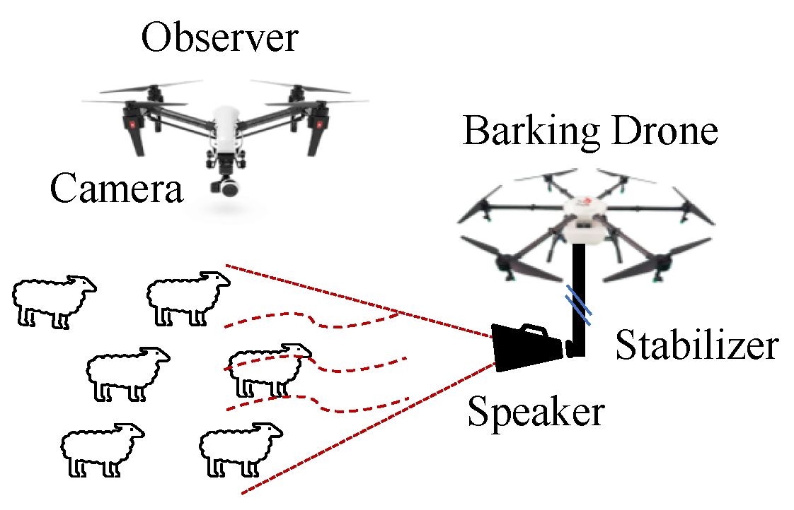
A drone of the second type is attached with a speaker that plays sheepdogs’ barking. The speaker should have a clear voice, abundant volume, relatively small size and low weight. There have been some drone digital voice broadcasting systems on the market. For example, the MP130 from Chengzhi [32] can broadcast the voice for 500 m with a weight of 550 g. Moreover, the speaker is designed to be mounted on a stabiliser attached to the drone, so that it can stably broadcast to a desired direction, no matter which direction the barking drone is moving towards. It is worth to mention that the speaker on current human-piloted barking drone is not mounted on the stabiliser, so we improved the design of the current barking drones.

The observer and the barking drones have the communication ability. The communication between them can be realised by 2.4 gigahertz radio waves, which is commonly used by different drone products. The communication is mainly unidirectional from the observer to the barking drones. Specifically, the observer monitors the locations of animals on the edge of the flock and sends them to the barking drones in the real-time. A typical application scenario of the proposed system is herding a large flock of animals with one observer and multiple barking drones. Figure 1 shows a schematic diagram of a basic unit of the drone herding system, with one operator and one barking drone.

Figure 1. A basic unit of the proposed drone herding system.

Limited battery life is always a problem of drones applications. Later we will show that the proposed herding system can usually accomplish the herding task in less than 50 min, which is the common endurance of some commercialised industrial drone products such as the DJI M300 [33] (Note that, such industrial drones usually cost thousands of US dollars each, i.e., might be cheaper than a fully trained sheepdog). Moreover, any drone in the system should be able to autonomously fly back to a ground drone base station to recharge the battery with automatic charging devices [34]. Besides, the advancement of solar-harvesting technology enables the drones to prolong the battery lifetime [35].

3. System Model and Problem Statement

In this section, we introduce the dynamics models of animal motion and drone motion. Then, we present the herding problem formulation and the preliminaries for designing drones motion controller.

3.1. Animal Motion Dynamics

Same as most research on robotic herding [20,27,36], we describe the dynamic of animal flocking by boids model based on Reynolds’ rules [37], which models the interaction of the agents based on attraction, repulsion and alignment models that are common in studies of collective animal behaviour. Field tests in [15] show that the boids model matches the behaviour of real flocks of sheep. The overall herd behaviour emerges from the decisions of individual members of the herd based on the four basic principles of collision avoidance, velocity matching (to nearby members of the herd), flock centring (the desire to be near the centre of the nearby members) and hazard avoidance. In detail, given the predefined constants $r_s$, $N_s$ and $r_a$, an animal under consideration behaves according to the following rules:

• If the distance to the barking drone is within $r_s$, then an animal will be repulsed directly away from the barking drone;
• An animal is attracted to the centre of mass of its $N_s$ nearest neighbours;
• Animals are also locally repulsed from each other, so that if two or more animals are within a distance of $r_a$ of each other there will be a repulsive force acting to separate them;
• Otherwise, an animal is semistationary with some small random movements.

Let unit vectors ${\overrightarrow{\aleph }}_d$, ${\overrightarrow{\aleph }}_L$, ${\overrightarrow{\aleph }}_r$, ${\overrightarrow{\aleph }}_i$ and ${\overrightarrow{\aleph }}_e$ denote the repulsive force from the barking drone to the animal, the attractive force to the centre of mass of the animal’s $N_s$ nearest neighbours, the repulsive force from other animals within a distance of $r_a$ of the animal, the inertial force to remain at the current location, and the noise element of the animal’s movement, respectively. Then, the animal’s moving direction vector $\overrightarrow{\aleph }$ is obtained by:

$$\overrightarrow{\aleph }={\eta }_d{\overrightarrow{\aleph }}_d+{\eta }_L{\overrightarrow{\aleph }}_L+{\eta }_r{\overrightarrow{\aleph }}_r+{\eta }_i{\overrightarrow{\aleph }}_i+{\eta }_e{\overrightarrow{\aleph }}_e,$$

(1)

where ${\eta }_d$, ${\eta }_L$, ${\eta }_r$, ${\eta }_i$, and ${\eta }_e$ are the weighting constants. Let $V_{\mathit{animal}}$ be the maximum speed of the animal.

3.2. Drone Motion Dynamics

In this paper, we assume the barking drones maintain at a fixed altitude that is relatively low to keep the barking drones close to the herding animals. With the fixed altitude, we study the 2D motion of a barking drone described by the following mathematical model. Let

$$\mathit{d}\left(t\right):=\left[x\right(t),y(t\left)\right]$$

(2)

be the 2D vector of the barking drone’s Cartesian coordinates. Then, the motion of the barking drone is described by the equations:

$$\dot{\mathit{d}}\left(t\right)=v\left(t\right)\mathit{a}\left(t\right),$$

(3)

$$\dot{\mathit{a}}\left(t\right)=\mathit{u}\left(t\right),$$

(4)

where $\mathit{a}\left(t\right)\in {\mathbb{R}}^2$, $\left|\mathit{a}\right(t\left)\right|=1$ for all t, $\mathit{u}\left(t\right)\in {\mathbb{R}}^2$, $v\left(t\right)\in \mathbb{R}$, and the following constraints hold:

$$\left|\mathit{u}\left(t\right)\right|\le U_{\mathit{max}},v\left(t\right)\in [0,V_{max}],$$

(5)

$$\left(\mathit{a}\right(t),\mathit{u}(t\left)\right)=0,$$

(6)

for all t. Here, $|·|$ denotes the standard Euclidean vector norm, and $(·,·)$ denotes the scalar product of two vectors. The scalar variable $v\left(t\right)$ is the speed or linear velocity of the barking drone, and the scalar $\mathit{u}\left(t\right)$ is applied to change the direction of the droneâ’s motion, given by $\mathit{a}\left(t\right)$. $v\left(t\right)$ and $\mathit{u}\left(t\right)$ are two control inputs in this model. $U_{max}$ and $V_{max}$ are constants depending on the manufacturing of the drone. The condition (6) guarantees that the vectors $\mathit{a}\left(t\right)$ and $\mathit{u}\left(t\right)$ are always orthogonal. Furthermore, $\dot{\mathit{d}}\left(t\right)$ is the velocity vector of the barking drone. The kinematics of many unmanned aerial vehicles can be described by the non-holonomic model (3)–(6); see, for example, [38] and references therein.

3.3. Problem Statement

Our goal is to navigate a network of barking drones to herd a flock of farm animals. A typical herding task consists of gathering and driving. In detail, we aim to navigate the barking drones to collect a flock of farm animals when they are too dispersed, namely gathering, and drive them to a designated location once they are aggregated, namely driving.

Let $\mathsf{\Phi }=\left\{{\mathit{\varphi }}_i\right\},i=1,\cdots ,n_s$ and $\mathcal{D}=\left\{{\mathit{d}}_j\right\},j=1,\cdots ,n_d$ be the sets of the two-dimensional (2D) positions of $n_s$ farm animals and $n_d$ barking drones, respectively. Let $C_o\in {\mathbb{R}}^2$ denote the position of the herding animals’ centroid. For gathering, the goal is to gather all the herding animals around until the distance between $C_o$ and any animal reaches a predefined constant $R_c$, that is,:

$$|{\mathit{\varphi }}_i{C}_o|⩽R_c,\forall i=1,\dots ,n_s.$$

(7)

After gathering, the animals need to be driven to a designated location such as the centre of a sheepfold. The barking drones have to keep the animals aggregated during driving. Let G be the designated location. Similar to gathering, the goal of driving is formulated as:

$$|{\mathit{\varphi }}_{i}G|⩽R_c,\forall i=1,\dots ,n_s.$$

(8)

3.4. Preliminaries

We now introduce the preliminaries for presenting the drones motion control algorithms, including the system’s available measurement and the drones’ motion restriction. During gathering, we use the convex hull of all the herding animals to describe the animals’ footprint.

Available measurement: We assume that at any time t, the observer has the measurements of the positions of the vertices of the convex hull of all the herding animals, described by $\mathcal{P}=\left\{P_i\right\},i=1,\cdots ,n_p$, and $n_p$ is the number of vertices of the convex hull, which is much smaller than $n_s$. Besides, we assume the observer can estimate $C_o$ with image processing techniques. The accurate real-time locations of the barking drones should also be available. In practice, the real-time drone locations can be provided by embedded GPS chips since the pastures are often open-air.

Definition 1.

The extended hull is a unique polygon surrounds the convex hull. The edges of the extended hull and the convex hull are in one-to-one correspondence, with each pair of the corresponding edges parallel to each other and maintaining the same fixed distance.

Let $\mathcal{E}=\left\{E_i\right\},i=1,\cdots ,n_e$ be the set of 2D positions of all the extended vertices in a counterclockwise manner, $n_e=n_p$. We now present the construction of the extended hull for a given convex hull of the herding animals. Let $P_i$ be the position of a convex hull vertex with two neighbour vertices $P_{i-1}$ and $P_{i+1}$. Construct parallel lines $l_1$ and $l_2$ of edges $P_i{P}_{i+1}$ and $P_i{P}_{i-1}$ on the periphery of the convex hull, respectively. Both the distance between $l_1$ and $P_i{P}_{i+1}$ and the distance between $l_2$ and $P_i{P}_{i-1}$ are $d_s$, where $d_s$ is the predefined drone-to-animal distance. Let $E_i$ be the position of the intersection of $l_1$ and $l_2$. Then, $E_i$ is the extended hull’s vertex corresponding to $P_i$, also called as the extended vertex of $P_i$. Let $L_1$ be the position of the intersection of $l_1$ and the extension line of $P_i{P}_{i-1}$. Let $L_2$ be the position of the intersection of $l_2$ and the extension line of $P_i{P}_{i+1}$, as shown in Figure 2. Naturally, $P_i{L}_1{E}_i{L}_2$ is a parallelogram. Let $\alpha$ denote $\angle L_1{P}_i{L}_2$. Then, we have:

$$cos\alpha =\frac{(\overrightarrow{P_i{P}_{i-1}},\overrightarrow{P_i{P}_{i+1}})}{|\overrightarrow{P_i{P}_{i-1}}\left|\right|\overrightarrow{P_i{P}_{i+1}}|},$$

(9)

$$\overrightarrow{P_i{L}_1}=\frac{d_s}{|cos\alpha |}·\frac{\overrightarrow{P_{i-1}{P}_i}}{|\overrightarrow{P_{i-1}{P}_i}|},$$

(10)

$$\overrightarrow{P_i{L}_2}=\frac{d_s}{|cos\alpha |}·\frac{\overrightarrow{P_{i+1}{P}_i}}{|\overrightarrow{P_{i+1}{P}_i}|}.$$

(11)

Figure 2. Illustration of the convex hull of the herding animals () and the corresponding extended hull.

Thus, given $P_{i-1}$, $P_i$ and $P_{i+1}$, $E_i$ can be computed by:

$$E_i=P_i+\overrightarrow{P_i{L}_1}+\overrightarrow{P_i{L}_2}.$$

(12)

Motion restriction: For the purpose of efficient gathering and avoiding to disperse any herding animals, all the barking drones are restricted to move only on the extended hull during gathering.

We assume that the spread range of the barking from the drone is fan-shaped, and only animals within this range will be affected by the repulsion of the barking drone. The intensity of barking outside this range is below the minimum level that can cause the evasive behaviour of the animal. We call this fan-shaped range as the barking cone, with the effective broadcasting angle $\beta$ and distance $R_b$, respectively. The number of repulsed animals of a barking drone will be influenced by four aspects: $\beta$, $R_b$, drone-to-animal distance $d_s$ and the distribution of animals. With the help of the stabiliser, the speaker should always face to $C_o$, as illustrated in Figure 3.

Figure 3. Illustration of the effective broadcasting angle $\beta$ and distance $R_b$ with (a) a small drone-to-animal distance $d_s$ and (b) a larger drone-to-animal distance $d_s$, under the same animals’ distribution. Here () stands for the animal repulsing by the barking drone (); () stands for the animal outsides the barking broadcasting range; () stands for $C_o$.

Remark 1.

Figure 3 also shows that a larger $d_s$ may lead to fewer animals repulsing by the barking drone with the same β, $R_b$ and animals’ distribution, if fewer animals locating near the edges of the convex hull. But if there are more animals concentrated near the edges, the situation may be reversed.

4. Drones Motion Control for Gathering

This section introduces the motion control algorithms for a network of barking drones to quickly accomplish the gathering task. We first introduce the algorithm for navigating the barking drones to fly to the extended hull and to fly on the extended hull in Section 4.1 and Section 4.2, respectively. Then, Section 4.3 presents the optimal positions (steering points) for the barking drones to efficiently gather animals, as well the collision-free allocation of the steering points. A flowchart of the proposed method is shown in Figure 4.

Figure 4. Overview of the proposed method.

Let A be any point on the plane of the extended hull. Let B be a vertex of the extended hull. We now introduce two guidance laws for navigating a barking drone from A to B in the shortest time:

• Fly to edge: navigate the barking drone from an initial position A to the extended hull in the shortest time. Note that the vertices of the extended hull can be moving. Let O denote the barking drone’s reaching point on the extended hull; see Figure 5.
  

  Figure 5. Illustration of the path planning for a barking drone from A to B, where A is a point on the plane of the extended hull, B is a vertex of the extended hull, O is the reaching point of the drone on the extended hull. The animals’ convex hull is denoted by blue lines. The green arrows and black arrows are the planned trajectories with a given clockwise and counterclockwise direction, respectively.
• Fly on edge: navigate the barking drone from O to B in the shortest time following a given direction, e.g., clockwise or counterclockwise, while keeping the barking drone on the extended hull. Since the drone has non-holonomic motion dynamics, it is allowed to move along a short arc when traveling between two adjacent edges, see Figure 5.

Note that A is not necessarily outside the extended hull. To avoid dispersing any herding animal, the speaker on the barking drone should be turned on only when it has arrived at the extended hull. Besides, if A is already on the extended hull, let $O=A$ and apply Fly on edge Guidance Law directly.

4.1. Fly to Edge Guidance Law

Let $w_1$ and $w_2$ be non-zero two-dimensional vectors, and $|w_1|=1$. Now introduce the following function $F(·,·)$ mapping from ${\mathbb{R}}^2\times {\mathbb{R}}^2$ to ${\mathbb{R}}^2$ as

$$\mathrm{F}\left(w_1,w_2\right):=\left\{\begin{array}{cc}0,\hfill & f\left(w_1,w_2\right)=0\hfill \\ {\left|f\left(w_1,w_2\right)\right|}^{-1}f\left(w_1,w_2\right),\hfill & f\left(w_1,w_2\right)\ne 0\hfill \end{array}\right.,$$

(13)

where $f\left(w_1,w_2\right):=w_2-\left(w_1,w_2\right)w_1$. In other words, the rule (14) defined in the plane of vectors $w_1$ and $w_2$. The resulted vector $F\left(w_1,w_2\right)$ is orthogonal to $w_1$ and directed “towards” $w_2$. Moreover, introduce the function $g\left(w_1,w_2\right)$ as follows

$$g\left(w_1,w_2\right):=\left\{\begin{array}{c}1,\left(w_1,w_2\right)>0,\hfill \\ -1,\left(w_1,w_2\right)\le 0,\hfill \end{array}\right.$$

(14)

We will also need the following notations to present the Fly to edge guidance law. At time t, let $E_{j+1}{E}_j$ be the extended hull edge that is the closest to the drone. We will show how to find $E_{j+1}{E}_j$ later. Let $q\left(t\right)\in {\mathbb{R}}^2$ denote the vector from vertex $E_{j+1}$ to $E_j$. Let $p\left(t\right)\in {\mathbb{R}}^2$ denote the vector from the vertex $E_{j+1}$ to the drone. Let O be the point on $E_{j+1}{E}_j$ that is the closest to the drone. Let $b\left(t\right)$ be the vector from the drone to O. If $(p,q)<0$, we have $O=E_{j+1}$ and $b\left(t\right)=-p\left(t\right)$, see Figure 6a. If $(p,q)>0$ and $\left|q\right|⩾\left|p\right|$, $b\left(t\right)$ is always orthogonal to $q\left(t\right)$. Let $o\left(t\right)$ be the vector from $E_{j+1}$ to O, see Figure 6b. $o\left(t\right)$ can be obtained by the following equation:

$$\left|o\left(t\right)\right|={\left|q\left(t\right)\right|}^{-1}(p\left(t\right),q\left(t\right)),$$

(15)

$$o\left(t\right)=\left|o\left(t\right)\right|·{\left|q\left(t\right)\right|}^{-1}q\left(t\right),$$

(16)

Figure 6. Illustration of (a) Fly to edge guidance with $(p,q)<0$; (b) Fly to edge guidance with $(p,q)<0$ and $\left|q\right|⩾\left|p\right|$; (c) Fly to edge guidance otherwise; (d) Fly on edge guidance navigates the drone from $\mathit{d}$ to $O^{*}$.

Otherwise, we have $O=E_j$ and $b\left(t\right)=q\left(t\right)-p\left(t\right)$, see Figure 6c. Given $p\left(t\right)$ and $q\left(t\right)$, we present the following Fly to edge guidance law:

$$b\left(t\right)=\left\{\begin{array}{c}-p\left(t\right),\mathrm{if}(p,q)<0,\hfill \\ o\left(t\right)-p\left(t\right),\mathrm{if}(p,q)>0\mathrm{and}\left|p\right|>\left|q\right|,\hfill \\ q\left(t\right)-p\left(t\right),\mathrm{otherwise},\hfill \end{array}\right.$$

(17)

$$\mathit{u}\left(t\right)=U_{\mathit{max}}g(\mathit{a}\left(t\right),b\left(t\right))F(\mathit{a}\left(t\right),b\left(t\right)),$$

(18)

$$v\left(t\right)=V_{\mathit{max}}g(\mathit{a}\left(t\right),b\left(t\right)).$$

(19)

The proposed Fly to edge guidance law belongs to the class of sliding-mode control laws (see, e.g., [39]). With the simple switching strategy, sliding mode control laws are quite robust and not sensitive to parameter variations and uncertainties of the control channel. Moreover, because the control input is not a continuous function, the sliding mode can be reached in finite time which is better than asymptotic behaviour, see for example, [39,40,41].

Assumption 1.

Let $\mathcal{X}\left(t\right)$ be the length of $E_i{E}_{(}i-1)$ at time t. Then ${\mathcal{X}}_1\le \mathcal{X}\left(t\right)\le {\mathcal{X}}_2$ for all t for some given constants $0<{\mathcal{X}}_1<{\mathcal{X}}_2$. Let $D_1$ and $D_2$ be some constants such that $0<D_1<D_2<{\mathcal{X}}_1$. Let $\delta \left(t\right)$ be the distance between the drone and $E_j$. $\delta \left(0\right)$ is the distance between A and $E_j$.

Assumption 2.

Let $\xi :=min\left\{\frac{{\mathcal{X}}_1-D_2}{D_2},\frac{D_1}{{\mathcal{X}}_2-D_1}\right\}$. Then

$$\xi V_{\mathit{max}}>\frac{D_1{V}_{animal}}{2{\mathcal{X}}_1},$$

(20)

$$U_{\mathit{max}}>\frac{V_{\mathit{animal}}}{{\mathcal{X}}_1},V_{\mathit{max}}>\frac{\left({\mathcal{X}}_2-D_1\right)V_{\mathit{animal}}}{{\mathcal{X}}_1},$$

(21)

$$D_1+\frac{\pi \left(V_{\mathit{max}}+V_{\mathit{animal}}\right)}{U_{\mathit{max}}}\le \delta \left(0\right)\le D_2-\frac{\pi \left(V_{\mathit{max}}+V_{\mathit{animal}}\right)}{U_{\mathit{max}}}.$$

(22)

Theorem 1.

Suppose that Assumptions 1 and 2 holds. Then, the guidance law (17), (18) and (19) navigate the barking drone from an initial position A to $E_{j+1}{E}_j$ and remains on $E_{j+1}{E}_j$ after arrival.

Remark 2.

It should be pointed out that Assumptions 1 and 2 are quite technical assumptions, which are necessary for a mathematically rigorous proof of the performance of the proposed guidance law. However, our simulations show that the proposed guidance law often performs well even in situations when Assumptions 1 and 2 do not hold.

Proof. 

From the definitions of $F\left(w_1,w_2\right)$ and $g\left(w_1,w_2\right)$, the guidance law (18), (19) turns the velocity vector $\dot{\mathit{d}}\left(t\right)$ towards $b\left(t\right)$. Moreover, Equation (17) gives that $b\left(t\right)$ is pointing from the drone to its closest point on $E_{j+1}{E}_j$, see Figure 6a–c. Furthermore, it follows from (22) together with Assumption 1 that there exists some time $t_{★}$ that for all $t\ge t_{★}$, the vectors $\dot{\mathit{d}}\left(t\right)$ and $b\left(t\right)$ are co-linear and $D_1\le \delta \left(t\right)\le D_2$. Introduce the function $Y\left(t\right)=\left|b\right(t\left)\right|$ is the distance between the drone’s current location and $E_{j+1}{E}_j$. Then, it follows from (20) of Assumption 2 and the inequality $D_1\le \delta \left(t\right)\le D_2$ that if $Y\left(t\right)>0$ then $\dot{Y}\left(t\right)<-\tau$ for some constant $\tau >0$. Therefore, there exists a time $t_a$ such that the drone’s current position belongs to $E_{j+1}{E}_j$ for all $t\ge t_a$. Moreover, (21) implies that for all $t\ge t_a$ the drone will remain in the sliding mode of the system (3), (4), (17), (18), (19) corresponding to the position of the drone on $E_{j+1}{E}_j$, and the and the vector $\dot{\mathit{d}}\left(t\right)$ orthogonal to $E_{j+1}{E}_j$. This completes the proof of Theorem 1.    □

Remark 3.

At time t, given $\mathit{d}\left(t\right)$ and E, calculate $b\left(t\right)$ for the barking drone to each edge of the extended hull. Then, the edge with the minimum $\left|b\right(t\left)\right|$ is the closest edge of the extended hull to the drone.

4.2. Fly on Edge Guidance Law

Before introducing the Fly on edge guidance law, we first present the edge sliding guidance law for a drone flying along an edge of the extended hull, with possibly moving vertices. At time t, let $E_{j+1}{E}_j$ be the edge that we want to keep the drone on. Let $O^{*}\in E_j{E}_{j+1}$ be the target position of the barking drone. Let $o^{*}\left(t\right)\in {\mathbb{R}}^2$ denote the vector from the drone to $O^{*}$, as shown in Figure 6d. We introduce $b^{*}\left(t\right)$ that is given by:

$$b^{*}\left(t\right)=b\left(t\right)+o^{*}\left(t\right).$$

(23)

Then, the edge sliding guidance law is as follows:

$$\mathit{u}\left(t\right)=U_{\mathit{max}}g(\mathit{a}\left(t\right),b^{*}\left(t\right))F(\mathit{a}\left(t\right),b^{*}\left(t\right)),$$

(24)

$$v\left(t\right)=V_{\mathit{max}}g(\mathit{a}\left(t\right),b^{*}\left(t\right)).$$

(25)

Theorem 2.

Suppose that Assumption 1 holds. Then the guidance law (23), (24) and (25) navigates the barking drone from $\mathit{d}\left(t\right)$ to $O^{*}$ along $E_{j+1}{E}_j$, and enables the drone to stay at $O^{*}$.

Note that, $b^{*}\left(t\right)$ consists of two vector components: $b\left(t\right)$ and $o^{*}\left(t\right)$. Where $b\left(t\right)$ is for keeping the drone on $E_{j+1}{E}_j$ and $o^{*}\left(t\right)$ is for navigating the drone to $O^{*}$. Thus, Theorem 2 can be proved similar to Theorem 1.

Suppose that the barking drone has arrived at the point O at time $t=t_0$. Introduce a direction index $\sigma =0$ for clockwise flying and $\sigma =1$ for counterclockwise flying. Given O, $\mathcal{E}$, B and $\sigma$, the Fly on edge guidance law solves for the barking drone’s control input $v\left(t\right)$ and $\mathit{u}\left(t\right)$ by commanding one of the two following motions.

4.2.1. TRANSFER

The drone flies to the adjacent edge in the given direction from its current location through a straight line and an arc. Consider that the drone flies from its current edge $E_{j-1}{E}_j$ to the adjacent edge $E_j{E}_{j+1}$. The drone first moves to $F_1\in E_{j-1}{E}_j$ following the edge sliding guidance law. Then, let $\mathit{u}\left(t\right)=U_{max}F(\mathit{a}\left(t\right),\mathit{e}\left(t\right))$ and $v\left(t\right)=V_{max}$, where $\mathit{e}\left(t\right):=\overrightarrow{\mathit{d}\left(t\right)C_t}$ denote the vector points from the drone’s current location to the turning centre $C_t$. The drone will turn with the minimum turning radius and arrives at $F_2\in E_j{E}_{j+1}$, as shown in Figure 7.

Figure 7. Illustration of the motion TRANSFER.

Let $\rho$ be the minimum turning radius of the drone. Let $\theta \in (0,\pi )$ denote the angle $\angle E_{j-1}{E}_j{E}_{j+1}$. $P_j$ is the convex hull vertex corresponding to $E_j$. Then, $F_1$ and $C_t$ can be computed by:

$$F_1=E_j+\frac{\overrightarrow{E_j{E}_{j-1}}}{|\overrightarrow{E_j{E}_{j-1}}|}·\frac{\rho }{tan\frac{\theta }{2}},$$

(26)

$$C_t=P_j+\frac{\overrightarrow{E_j{P}_j}}{|\overrightarrow{E_j{P}_j}|}·\frac{\rho -d_s}{sin\frac{\theta }{2}},$$

(27)

where $d_s$ denotes drone-to-animal distance, as defined above. $\theta$ can be obtained from the equation similar to (10). To avoid dispersing any animals, the turning trajectory should not touch the convex hull of the animals, which always holds in the case of $d_s>\rho$. If $d_s\le \rho$, the following inequalities need to be satisfied:

$$\begin{array}{c}\left|C_t{P}_j\right|=\frac{\rho -d_s}{sin\frac{\theta }{2}}<\rho ,\hfill \\ \Rightarrow sin\frac{\theta }{2}>1-\frac{d_s}{\rho },\hfill \\ \Rightarrow \theta >2arcsin\left(1-\frac{d_s}{\rho }\right).\hfill \end{array}$$

(28)

Remark 4.

If (28) does not hold, the drone directly flies to $E_j$ following the edge sliding guidance law, then stops and changes direction to $\overrightarrow{E_j{E}_{j+1}}$, which is slower than along the arc trajectory. An isolated animal far away from all the other animals may cause a very small θ and lead to this problem.

4.2.2. BRAKE

If the drone has arrived at an edge $E_{b}B$, where $E_b\in \mathcal{E}$ is the closest vertex of B on the opposite of the direction indicated by $\sigma$, then the drone flies to a point B following the edge sliding guidance law. Let $E_0^{\prime }\in \mathcal{E}$ be the closest vertex to the drone opposite to the given direction. Let $\mathcal{H}\subseteq \mathcal{E}$ be the set of vertices locating between O and B along the given direction.

We are now in a position to present the Fly on edge guidance law, as shown in Algorithm 1. Specifically, the drone approaches the edge $E_{b}B$ that contains the destination B by performing TRANSFER multiple times. Afterwards, the drone starts BRAKE once $\mathcal{H}$ is found to be an empty set (i.e., $\mathcal{H}=\varnothing$), which means the drone has arrived at $E_{b}B$. The drone will then reaches B through BRAKE. The presented guidance law is designed to navigate the barking drone from any point on the extended hull to a selected vertex following a given direction, and stop the drone at the selected vertex.

Algorithm 1: Fly On Edge Guidance Law.

Input O, $\mathcal{E}$, B, $\sigma$, $\rho$ 1:  Find $E_0^{\prime }$ and $\mathcal{H}$, if $\mathcal{H}=\varnothing$, go to line 4; 2:  [$v\left(t\right)$, $\mathit{u}\left(t\right)$] = TRANSFER($E_0^{\prime }$, $\mathcal{H}$); 3:  Repeat lines 1, 2; 4:  [$v\left(t\right)$, $\mathit{u}\left(t\right)$] = BRAKE($E_0^{\prime }$, B).

4.3. Selection and Allocation of Steering Points

We now find the optimal positions for the barking drones to effectively gather animals. Aiming to minimise the maximum animal-to-centroid distance in the shortest time, at any time t, we choose the animals with the largest animal-to-centroid distance as the target animals. These animals are also the convex hull vertices that are farthest to $C_o$. Since the barking drones have their motions restricted on the extended hull, we select the extended hull vertices corresponding to the target animals as the optimal drone positions for steering the target animals to approach $C_o$. From now on, we call these corresponding extended hull vertices the steering points, denoted by the set $\mathcal{S}=\left\{{\mathbf{s}}_j\right\},j=1,\cdots ,n_d$, $\mathcal{S}\subseteq \mathcal{E}$.

Remark 5.

For a large flock of animals, $n_e\ge n_d$ holds generally. In the cases of $n_e<n_d$, let $n_d-n_e$ barking drones that are far from the steering points quit the gathering task, stand by at their current locations. These drones may rejoin the gathering task when $n_e$ increases afterwards.

Definition 2.

The allocation of steering points specifies which drone goes to which steering point through which direction, that is, clockwise or counterclockwise.

The optimal allocation of steering points should meet the following two requirements:

• No collision happens when each drone is flying to its allocated steering point along the extended hull;
• With requirement 1 met, the maximum travel distance of the drones is minimised.

Suppose that all the drones have arrived at the extended hull at time $t=t_1$. We relabel the drones so that the index of the drone increases in the counterclockwise direction. Let M be the perimeter of the extended hull. Imagine that we disconnect the extended hull from the position of the first drone, that is, ${\mathit{d}}_1\left(t\right)$. Then, ’straighten’ the extended hull into a straight line segment with a length of M, so that $\mathcal{D}$, $\mathcal{S}$ and $\mathcal{E}$ become the points on the line segment. Based on this line segment we build a one-dimensional (1D) coordinate axis denoted as the z axis. Let $\mathcal{Z}=\left\{z_j\right\},j=1,\cdots ,n_d$ be the 1D coordinates of the drones’ positions on the z axis. Let $z_1=0$ be the origin. We have $z_j<z_{j+1},j=1,\cdots ,n_d-1$, as shown in Figure 8a. It can be seen that the left and right flying on the z axis corresponding to counterclockwise and clockwise flying on the extended hull, respectively.

Figure 8. The examples of (a) drones’ positions on the z axis, (b) steering points’ positions on the z axis, (c) steering points on the $z^{*}$ axis, and (d) drone’s positions, steering points’ positions and travel routes on the $z^{*}$ axis. Here () stands for $z_j$, () stands for $z_j^{\prime }$, () stands for $z_j^{*}$, and the blue arrows stand for the drones’ travel routes.

We will also need the following notations to present our algorithm. Let ${\mathcal{S}}^{\prime }=\left\{{\mathbf{s}}_j^{\prime }\right\},j=1,\cdots ,n_d$ be a set of allocated steering points with a corresponding z axis coordinates set ${\mathcal{Z}}^{\prime }=\left\{z_j^{\prime }\right\},j=1,\cdots ,n_d$, as shown in Figure 8b. ${\mathcal{Z}}^{\prime }$ is the destination of the drones on the z axis. Note that, $z_j^{\prime }<z_{j+1}^{\prime },j=1,\cdots ,n_d-1$ may not hold. Let $\mathsf{\Gamma }=\left\{{\gamma }_j\right\},j=1,\cdots ,n_d$ be the set of the drones’ travel distances for reaching their allocated steering points. We now define three variables ${\sigma }_j$, ${\lambda }_j^R$ and ${\lambda }_j^L\in \left\{0,1\right\}$ to indicate the flying direction and extent of drone j. Specifically, let ${\sigma }_j=1$ if drone j reaches $z_j^{\prime }\left(t\right)$ by right flying on the z axis, and ${\sigma }_j=0$ if drone j reaches $z_j^{\prime }\left(t\right)$ by left flying on the z axis. Furthermore, let ${\lambda }_j^R=1$ if drone j will pass $z=0$ by right flying to reach $z_j^{\prime }\left(t\right)$, and ${\lambda }_j^R=0$ otherwise. Similarly, let ${\lambda }_j^L=1$ if drone j will pass $z=0$ by left flying to reach $z_j^{\prime }\left(t\right)$, and ${\lambda }_j^L=0$ otherwise. Let $\mathsf{\Sigma }=\left\{{\sigma }_j\right\}$, ${\mathsf{\Lambda }}^L=\left\{{\lambda }_j^L\right\}$ and ${\mathsf{\Lambda }}^R=\left\{{\lambda }_j^R\right\},j=1,\cdots ,n_d$ be the sets of ${\lambda }_j^L$ and ${\lambda }_j^R$, respectively. Given $z_j$, $z_j^{\prime }$ and ${\sigma }_j$, ${\lambda }_j^L$ and ${\lambda }_j^R$ can be computed by:

$${\lambda }_j^L=\left\{\begin{array}{c}1,\mathrm{if}{z}_j^{\prime }>z_j\mathrm{and}{\sigma }_j=0,\hfill \\ 0,\mathrm{otherwise},\hfill \end{array}\right.$$

(29)

$${\lambda }_j^R=\left\{\begin{array}{c}1,\mathrm{if}{z}_j^{\prime }<z_j\mathrm{and}{\sigma }_j=1,\hfill \\ 0,\mathrm{otherwise}.\hfill \end{array}\right.$$

(30)

The main notations are listed in Table 1. Since the line segment $z=[0,M]$ is generated by straightening the enclosed extended hull, the drones passed $z=0$ by left flying will appear on the right side of the line segment, and the drones passed $z=M$ by right flying will be appear on the left side of the line segment. We now imagine extending the line segment $z=[0,M]$ to $z=[-M,2M]$ and build another 1D coordinate $z^{*}$ axis as shown in Figure 8c. On the $z^{*}$ axis, the drones passed $z^{*}=0$ by left flying will not appear on the right side of the line segment, but will appears on $z^{*}=[-M,0]$, and the drones passed $z^{*}=M$ by right flying will be appear on $z^{*}=[M,2M]$. Let ${\mathcal{Z}}^{*}=\left\{z_j^{*}\right\},j=1,\cdots ,n_d$ be the 1D coordinates set on the $z^{*}$ axis corresponding to ${\mathcal{Z}}^{\prime }$. Then, the mapping between ${\mathcal{Z}}^{*}$ and ${\mathcal{Z}}^{\prime }$ is obtained by:

$$z_j^{*}=\left\{\begin{array}{c}{z}_j^{\prime }-{\lambda }_j^{L}M,\mathrm{if}{\sigma }_j=0,\hfill \\ z_j^{\prime }+{\lambda }_j^{R}M,\mathrm{if}{\sigma }_j=1.\hfill \end{array}\right.$$

(31)

Table 1. Notations and Descriptions.

Notation	Description
M	Perimeter of the extended hull.
$\mathcal{D}=\left\{{\mathit{d}}_j\right\}$	Set of the drones’ 2D positions.
$\mathcal{Z}=\left\{z_j\right\}$	Set of the z coordinates of $\mathcal{D}$.
$\mathcal{S}=\left\{{\mathbf{s}}_j\right\}$	Set of the steering points’ 2D positions.
${\mathcal{S}}^{\prime }=\left\{{\mathbf{s}}_j^{\prime }\right\}$	Set of the allocated steering points’ 2D positions.
${\mathcal{Z}}^{\prime }=\left\{z_j^{\prime }\right\}$	Set of the z coordinates of ${\mathcal{S}}^{\prime }$.
${\mathcal{Z}}^{*}=\left\{z_j^{*}\right\}$	Set of the $z^{*}$ coordinates of ${\mathcal{Z}}^{\prime }$.
$\mathsf{\Gamma }=\left\{{\gamma }_j\right\}$	Set of drones’ travel distances .
$\mathsf{\Sigma }=\left\{{\sigma }_j\right\}$	Set of drones’ flying directions.
${\mathsf{\Lambda }}^L=\left\{{\lambda }_j^L\right\}$	Set of the indicators of passing $z=0$ by right flying.
${\mathsf{\Lambda }}^R=\left\{{\lambda }_j^R\right\}$	Set of the indicators of passing $z=0$ by left flying.

If place $\mathcal{Z}$ on the $z^{*}$ axis, as shown in Figure 8c, the travel route of any drone j will be $\overrightarrow{z_j{z}_j^{*}}$. We obtain the expression for the travel distances ${\gamma }_j$ as follows:

$${\gamma }_j=\left\{\begin{array}{c}{z}_j-z_j^{*},\mathrm{if}{\sigma }_j=0,\hfill \\ z_j^{*}-z_j,\mathrm{if}{\sigma }_j=1.\hfill \end{array}\right.$$

(32)

Then, the steering points allocation optimization problem is formulated as follows:

$$\underset{S^{\prime },\mathsf{\Sigma }}{min}\underset{j=1,\cdots ,n_d}{\mathit{max}}{\gamma }_j,$$

(33)

s.t.

$$0<z_{n_d}^{*}-z_1^{*}<M,$$

(34)

$$z_j^{*}<z_{j+1}^{*},j=1,\cdots ,n_d-1,$$

(35)

where (33) minimises the travel distance of the drone farthest to its allocated steering point.

Assumption 3.

All the drones start flying to their allocated steering points at the same time, follow the proposed Fly on edge guidance law.

Theorem 3.

Suppose that Assumption 2 holds. Then, (34), (35) guarantees that no collision happens when the drones are flying to their allocated steering points.

Proof. 

Suppose that all the drones start flying to their steering points at time $t=t_0$. Let $t=t_f^j$ be the time of drone j arrives at its steering point, that is, $z_j^{*}\left(t\right)$. From (14) and (25), at any time $t=t_s\in [t_0,t_f^j]$, drone $j\in \left\{2,\cdots ,n_d-1\right\}$ has:

$$|v\left(t_s\right)|=V_{max}.$$

(36)

From the proof of Theorem 1, $b\left(t\right)$ is always been minimised after drone j arrived at the extended hull. Since drone j is moving from $z_j\left(t_0\right)$ to $z_j^{*}$ along the z axis, it can be obtained from (23) and (3) that

$$b^{*}\left(t_s\right)=z_j^{*}-z_j\left(t_s\right),$$

(37)

$$z_j\left(t_s\right)=z_j\left(t_0\right)+(t_s-t_0)V_{max},$$

(38)

$$z_j^{*}=z_j\left(t_0\right)+(t_f^j-t_0)V_{max}.$$

(39)

Then, the distance between drone j and drone $j+1$ at time $t=t_s\in [t_0,\max (t_f^j,t_f^{j+1})]$ can be computed by

$$z_{j+1}\left(t_s\right)-z_j\left(t_s\right)=\left\{\begin{array}{c}\begin{array}{c}\hfill z_{j+1}\left(t_0\right)-z_j\left(t_0\right),\mathrm{if}{t}_s\le min(t_f^j,t_f^{j+1}),\\ \hfill z_{j+1}\left(t_s\right)-z_j^{*},\mathrm{if}{t}_f^j\le t_f^{j+1}\mathrm{and}{t}_f^j<t_s\le t_f^{j+1},\\ \hfill z_{j+1}^{*}-z_j\left(t_s\right),\mathrm{if}{t}_f^j>t_f^{j+1}\mathrm{and}{t}_f^{j+1}<t_s\le t_f^j.\end{array}\hfill \end{array}\right.$$

(40)

Since $z_j<z_{j+1},j=1,\cdots ,n_d-1$, it can be concluded from (35), (38), (39) and (40) that

$$z_{j+1}\left(t_s\right)-z_j\left(t_s\right)>0,t_s\in [t_0,\max (t_f^j,t_f^{j+1})]$$

(41)

Which means drone $j\in \left\{2,\cdots ,n_d-1\right\}$ will not collide with drone $j+1$ before they arrived at their steering points. Moreover, the actual distance $|z_1{z}_{n_d}|$ between drone 1 and drone $n_d$ is given by

$$|z_1{z}_{n_d}|=\left\{\begin{array}{c}\begin{array}{c}\hfill z_{n_d}\left(t_s\right)-z_1\left(t_s\right),\mathrm{if}{z}_{n_d}\left(t_s\right)-z_1\left(t_s\right)\le M/2,\\ \hfill M-(z_{n_d}\left(t_s\right)-z_1\left(t_s\right)),\mathrm{if}{z}_{n_d}\left(t_s\right)-z_1\left(t_s\right)>M/2.\end{array}\hfill \end{array}\right.$$

(42)

Given (34), $|z_1{z}_{n_d}|>0,t_s\in [t_0,\mathit{max}(t_f^1,t_f^{n_d})]$ can be proved similarly. Therefore, (34) guarantees that drone 1 will not collide with drone $n_d$, and (35) guarantees that each drone will not collide with their neighbours. This completes the proof of Theorem 3.    □

Remark 6.

For $n_d$ drones, $n_d$ steering points and two possible directions for each drone, the number of possible allocations is $N=n_d!2^{n_d}$.

Since $n_d$ is often a limited number, N will be limited as well. Therefore, the optimal allocation can be found by generating and searching all the possible allocations. We are now in a position to present the algorithm to find the optimal steering points allocation, as shown in Algorithm 2.

Algorithm 2: Optimal Steering Points Allocation.

Input $n_d$, E, D 1:  Find $\mathcal{S}\in \mathcal{E}$; 2:  Calculate $\mathcal{Z}$ from $\mathcal{D}$ and $\mathcal{E}$; 3:  Generate possible allocations ${({\mathcal{S}}^{\prime },\mathsf{\Sigma })}^k,k=1,\cdots ,N$; 4:  For each ${({\mathcal{S}}^{\prime },\mathsf{\Sigma })}^k$, calculate ${({\mathcal{Z}}^{*},\mathsf{\Gamma })}^k$; 5:  Solve (29)–(31) by searching ${({\mathcal{Z}}^{*},\mathsf{\Gamma })}^k,k=1,\cdots ,N$.

Suppose that the gathering task starts at $t=0$. The proposed herding system first navigates all the barking drones to the extended hull by Fly to edge guidance law. Then, the system calculates the optimal steering points allocation after every sampling time $\mathsf{\Delta }$ and navigates the barking drones to their allocated steering points by Fly on edge guidance law, until (7) is satisfied, that is, $|{\mathit{\varphi }}_i{C}_o|⩽R_c,\forall i=1,\dots ,n_s$. It is worth mentioning that the optimal allocation may change before some drones arrived at their allocated steering points due to the animals’ movement. The gathering task, however, will be interrupted. Because as long as the barking drones are flying on the extended hull, the animals inside the drones’ barking cone will be repulsed to move towards $C_o$.

5. Drones Motion Control for Driving

Suppose that (7) is satisfied at $t=t_g$, the goal is then transferred to drive the gathered animals to a desired location, for example, the centre of a sheepfold. The convex hull of the gathered animals will be close to a circle. For simplicity, from now on, we use the smallest enclosing circle to describe the footprint of the gathered animals. Let $R_c^{\prime }$ and $C_o^{\prime }$ be the radius and centre of the animals’ smallest enclosing circle during driving, respectively. Similar to the definition of the extended hull, we define the extended circle as a circle with a larger radius $R_e:=R_c^{\prime }+d_s$ centred at $C_o^{\prime }$.

According to (7), $R_c^{\prime }=R_c$ and $C_o^{\prime }=C_o$ when $t=t_g$. Imagine a point $C_{*}\in C_{o}G$ is moving from $C_o$ to G with a constant speed $V_{driving}\le V_{animal}$ when $t_g\le t\le t_d$, where $t_d$ denotes the time when the driving task is finished (i.e., (8) is satisfied). Given $C_o=[x_o,y_o]$ and $G=[x_g,y_g]$, $C_{*}=[x_{*},y_{*}]$ can be computed by:

$$\left[\begin{array}{c}{x}_{*}\hfill \\ y_{*}\hfill \end{array}\right]=\left[\begin{array}{c}{x}_0\hfill \\ y_0\hfill \end{array}\right]+V_{driving}\left(t-t_g\right)\frac{\overrightarrow{CG}}{|\overrightarrow{CG}|},t_g\le t\le t_d.$$

(43)

We aim to drive the animals so that $C_o^{\prime }$ can follow $C_{*}$ moving from $C_o$ to G, with $V_{driving}$ as the driving speed. Note that, a smaller $V_{driving}$ is preferred for a larger animals’ number $n_s$, because a larger flock of animals tend to move slower. To this end, we adopt a side-to-side movement for the baking drones, which is a common animal driving strategy that can also be seen in [15,42], and so forth. Let $l_g$ be the perpendicular line of $C_{o}G$ that passes $C_{*}$. Let $\mathcal{L}$ be the semicircle of the extended circle cut by $l_g$ that is farther to G; see Figure 9. Let $\mathcal{Q}=\left\{Q_j\right\},j=1,\cdots ,n_d+1$ be the set of points that evenly distributed on $\mathcal{L}$. Each drone j is then deployed to fly on $\mathcal{L}$ with $Q_j$ and $Q_{j+1}$ as its start and end points, respectively, as shown in Figure 9. With $C_{*}$ approaching G, the side-to-side movements of the barking drones can ’push’ the animals to approach G while keeping them aggregated.

Figure 9. Barking drones deployment for animal driving, where the star marker stands for the designated location G; the red dot stands for $C_o^{\prime }$. The dark red arrows stand for the side-to-side trajectories of the barking drones.

Given $R_e$ and $C_{*}=[x_{*},y_{*}]$, $Q_j:=[x_j^q,y_j^q],j=1,\cdots ,n_d+1$ can be computed by solving the following equations:

$${\left(x_j^q-x_{*}\right)}^2+{\left(y_j^q-y_{*}\right)}^2=R_e^2,$$

(44)

$$k_1\left(x_{1,n_d+1}^q-x_{*}\right)+k_2\left(y_{1,n_d+1}^q-y_{*}\right)=0.$$

(45)

If $n_d$ is an odd number,

$$\begin{array}{cc}\hfill k_1& \left(x_{j,n_d-j+2}^q-x_{*}\right)+k_2\left(y_{j,n_d-j+2}^q-y_{*}\right)\hfill \\ \hfill & =\mu R_{e}cos\left(\frac{\pi }{2}+\psi (j-1)\right),j=2,\dots ,\frac{n_d+1}{2}.\hfill \end{array}$$

(46)

If $n_d$ is an even number,

$$\begin{array}{cc}\hfill k_1& \left(x_{j,n_d-j+2}^q-x_{*}\right)+k_2\left(y_{j,n_d-j+2}^q-y_{*}\right)\hfill \\ \hfill & =\mu R_{e}cos\left(\frac{\pi }{2}+\psi (j-1)\right),j=2,\dots ,\frac{n_d}{2},\hfill \end{array}$$

(47)

$$k_1\left(x_{n_m}^q-x_{*}\right)+k_2\left(y_{n_m}^q-y_{*}\right)=-\mu R_e,$$

(48)

where

$$\psi =\frac{\pi }{n_d},$$

(49)

$$k_1=x_g-x_{*},k_2=y_g-y_{*},$$

(50)

$$\mu =\sqrt{{k_1}^2+{k_2}^2}.$$

(51)

$$n_m=\frac{n_d}{2}+1.$$

(52)

Specifically, once (7) is satisfied, all the barking drones immediately fly to the extended circle following the guardians law similar to the Fly to edge introduced in Section 4.1. It is worth mentioning that the extended polygon is inscribed in the extended circle, so the process of the drones flying to their closest point on the extended circle will not disperse any animal. After reaching the extended circle, the barking drones fly to their allocated start points in ${\mathcal{Q}}^{*}=\left\{Q_j\right\},j=1,\cdots ,n_d\in \mathcal{Q}$ following the guardians law similar to the Fly on edge introduced in Section IV.2. The allocation of ${\mathcal{Q}}^{*}$ can be found by the algorithm similar to Algorithm 2 introduced in Section IV.3. Then, drone j continuously flies between $Q_j$ and $Q_{j+1}$ along $\mathcal{L}$, as shown in Figure 9, until (8) is satisfied.

6. Results

In this section, the performance of the proposed method is evaluated using MATLAB. Each simulation runs for 20 times. The animal motions dynamic parameters are chosen based on the field tests with real sheep conducted by [15], as shown in Table 2. Table 2 also shows some parameters of the barking drones, if not specified in the following part.

Table 2. Simulation Parameter Values.

Parameters	Values	Parameters	Values
$N_s$	20	$r_a$	2 m
${\eta }_d$	1	${\eta }_L$	1.05
${\eta }_r$	2	${\eta }_i$	0.5
${\eta }_e$	0.3	$\mathsf{\Delta }$	0.2 s
$V_{max}$	25 m/s	$U_{max}$	5 m/s2
$V_{animal}$	4 m/s	$\beta$	$\frac{2\pi }{3}$
$R_b$	100 m	$d_s$	30 m
$n_s$	200, 1000	$R_c$	60, 110 m
$V_{driving}$	3.8 m/s, 1.9 m/s	$n_d$	4

For comparison, we introduce an intuitional collision-free method as the benchmark method. Specifically, the benchmark method divides the extended hull into $n_d$ segments with the same length at any time during gathering. Each drone is allocated to a segment and do the aforementioned side-to-side movement on the extended hull, until (7) is satisfied. The benchmark method adopts the same driving strategy as the proposed method. We consider that the animals are randomly distributed in an area with the size of 1200 m by 600 m as the initial field.

We first present some illustrative results showing 4 barking drones on two cases herding 200 and 1000 animals, respectively; see https://youtu.be/KMWxrlkU6t0, (accessed on 8 december 2021) and https://youtu.be/KPGrAcgPH8Q, (accessed on 8 december 2021). We can observe that the proposed method completes the gathering task in 9.5 min for the instance with 200 animals and 10.1 min for the case with 1000 animals. The total time for gathering and driving are 15 and 18.2 min for these cases. However, the benchmark method uses about 4.9 and 4.1 more minutes to complete these missions. Figure 10a shows how the animals’ footprint radius changes with time t for these cases. We also present snapshots when $t=0$, $t=5$ and $t=8$ min for the case of 1000 animals in Figure 10b–f.

Figure 10. (a) Animals’ footprint radius versus time t for herding 200 and 1000 animals with 4 barking drones using both the proposed and the benchmark method; (b) Initial distribution of the 1000 animals; (c–f) snapshots of the 1000 animals at $t=5,8$ min for both methods.

Interestingly, Figure 10a reveals that the difference between the time of gathering 200 animals and 1000 animals is not that obvious, with both the proposed method and the benchmark method. The proposed method, however, can always use less time to complete the gathering mission. This is because that the proposed method always chases and repulses the animals that are farthest to the centre, while the benchmark method is repulsing the animals indiscriminately. Therefore, the animals’ footprint with the proposed method becomes increasingly round-like during shrinking, while animals’ footprint with the benchmark method becomes long and narrow. This fact can be observed by comparing Figure 10c,e, and Figure 10d,f.

Note that, the time consumption of flying to the edge and the driving task mainly depend on the initial locations of the drones and the animals. From now on, we focus on evaluating the average gathering time after the drones have arrived on the extended hull. The aforementioned minor difference between herding 200 and 1000 animals is very likely because that the gathering time is strongly correlated with the size of the initial field, rather than the number of the animals. To confirm this, we change the initial field into square and investigate the relationship between the gathering time and the length of the initial square field; see Figure 11a. It reveals that the average gathering time increases significantly with the initial square field length. This supports the guess that the gathering time is strongly correlated with the size of the initial field. The reason is also that the gathering time mainly depends on the movement of the animals on the edge, and particularly the travelling time for them to move to the area close to $C_o$. With fixed $V_{animal}$ and the same repulsion from the barking drones, the travelling distances of these animals are dominated by the size of the initial field. Moreover, Figure 11a shows that the difference between the gathering time of the benchmark method and the proposed method increases with the initial square field length. It means the benchmark method is more ‘sensitive’ to the varying length of the initial square field. We further investigate the relationship between the gathering time and the the number of barking drones $n_d$; see Figure 11b. Not surprisingly, the average gathering time decreases significantly with the increase of $n_d$ for both methods. Besides, Figure 11b shows that the superiority of the proposed method becomes more obvious with $n_d$ increases when $n_d\ge 4$.

Figure 11. Comparisons of the average gathering time for different values of (a) length of the initial square field; (b) number of barking drones $n_d$.

Next, we investigate the impact of the drone speed and animal speed on the gathering time; see Figure 12. Figure 12a shows that slower drones will lead to a higher average gathering time, especially when the maximum drone speed $V_{max}<15$ m/s, for both the benchmark method and the proposed method. Moreover, the average gathering time of the benchmark method is more ‘sensitive’ to $V_{max}$ when $V_{max}<15$ m/s. In addition, in our simulations, drones with $V_{max}\le 10$ m/s cannot accomplish the gathering task using the benchmark method. In the implementation of the proposed method, drones with $V_{max}>15$ m/s is preferable. Furthermore, the average gathering time of the proposed method reduces with $V_{max}$ increases, the percentage of the reduction, however, is not significant when $V_{max}>30$ m/s. Figure 12b shows that animals with higher maximum speed $V_{animal}$ can be gathered in a shorter time. Particularly, with the proposed method, the average gathering time reduces around $38\%$ (from 14.7 min to 9.1 min) when $V_{animal}$ increases $150\%$ (from 2 m/s to 5 m/s). For the benchmark method, the average gathering time reduces around $39\%$ (from 20.8 min to 12.7 min). Therefore, the reduction of average gathering time is much slower than the increase of $V_{animal}$ when 2 m/s $\le V_{animal}\le 5$ m/s, for both methods.

Figure 12. Comparisons of the average gathering time for different values of (a) the maximum drone speed $V_{\mathit{max}}$; (b) the maximum animal speed $V_{animal}$.

We investigate impact of the barking cone radius $R_b$, the drone-to-animal distance $d_s$, and angle of barking cone $\beta$ on the gathering time; see Figure 13. Figure 13a presents the relationship between the barking radius $R_b$ and the gathering time with 200 animals and 1000 animals, respectively. We can observe that increasing $R_b$ will accelerate the gathering when $R_b\le 100$ m. But when $R_b>100$ m, the average gathering time increases with $R_b$, which is contradictory to our expectation. One possible reason is that the gathering time mainly depends on the animals on the edges. If $R_b$ is too lager, it may cause the mutual interference between the repulsive forces inflicted by the barking drones, which may pull down the gathering. Moreover, Figure 13a shows that the proposed method is more ‘sensitive’ to $R_b$ when gathering more animals with $R_b\le 100$ m. This is because that the proportion of the repulsed animals near the edges tend to be less when $n_s$ increases, for a fixed $R_b$.

Figure 13. Comparisons of the average gathering time for different values of (a) barking cone radius $R_b$; (b) drone-to-animal distance $d_s$; (c) angle of barking cone $\beta$.

Figure 13b suggests that the average gathering time decreases with $d_s$ increases when $d_s\le 30$ m. One possible reason is that more animals will be repulsed to the directions that are not point to the centre if $d_s$ is too small, since the repulsive force from the barking drone is point to the opposite of it and the barking zone is fan-shaped. This result is also considered the interference. However, increasing $d_s$ will decelerate the gathering when $d_s>30$ m, and this becomes more obvious with more animals. It is reasonable because increasing $d_s$ is almost equivalent to decreasing $R_b$ when $R_b$ is fixed.

Figure 13c indicates that the gathering time of the proposed method is significantly less than the one of the benchmark method among $\beta =\pi /2,2\pi /3$ and $3\pi /4$ with 200 animals and 1000 animals. It can also be seen from Figure 13c that the gathering time does not show monotonicity with the increase of $\beta$. The gathering time with $\beta =2\pi /3$, however, is slightly less than the cases with $\beta =\pi /2$ and $3\pi /4$, for both the proposed method and the benchmark method.

We are also interested in the impacts of the measurement errors from the ‘observer’ on our method. We add random noise to the measured positions of the animals, and the amplitude of the noise is from 2 to 10 m. We conduct 20 simulations with 200 animals and 1000 animals independently for each value with $d_s=20$ m. The results are as shown in Figure 12. Under the measurement error, the average impact on the gathering time is relatively small. Figure 12 shows that the average gathering time increased slightly with the measurement error increases from 2 to 10 m for both cases. For example, from no measurement error to 10 m error, the average gathering time for 1000 animals increased from 11.7 min to 12.6 min. The difference is less than 1 min. Moreover, the impact of measurement errors on the average gathering time is less significant in the case of 200 animals (see Figure 14).

Figure 14. Impact of measurement errors.

In summary, we present computer simulation results in this section to demonstrate the performance of the proposed method. These results confirm that the proposed method can efficiently herd a large number of farm animals and outperform the benchmark method. By investigating the impact of the system parameters we can obtain that higher speed of drones leads to shorter gathering time. The barking cone radius $R_b$ and the drone-to-animal distance $d_s$ also significantly affect the gathering time. The optimal values of them can be obtained via experiments on real animals.

7. Conclusions

In this paper, we proposed a novel robotic herding system based on autonomous barking drones. We developed a collision-free sliding mode based motion control algorithm, which navigates a network of barking drones to efficiently collect a flock of animals when they are too dispersed and drive them to a designated location. Simulations using a dynamic model of animal flocking based on Reynolds’ rules showed the proposed drone herding system can efficiently herd a thousand of animals with several drones. A unique contribution of this paper is the proposal of the first prototype of herding a large flock of farm animals by autonomous drones. The future work is to conduct experiments on real farm animals to test the proposed method. Moreover, the sound from drones may have some unknown effect on the animals and their responses. The study of such an aspect can also be carried out in field experiments.