New Analytical Solutions for Time-Fractional Stochastic (3+1)-Dimensional Equations for Fluids with Gas Bubbles and Hydrodynamics

Abstract

This paper explores the effects of spatial fractional derivatives and the multiplicative Wiener process on the analytical solutions for (3+1)-dimensional fractional stochastic equations for fluids with gas bubbles. We study the bifurcation of the analytical solutions and introduce new fractional stochastic solutions. We also discuss how the solutions differ depending on the initial conditions. The new solutions are notably more beneficial and impactful for understanding various, significant, and incredibly hard physical phenomena due to the significance of the modified fractional stochastic (3+1)-dimensional equations for fluids with gas bubbles and hydrodynamics. We also discuss the effects of the fractional order and the Wiener process on the obtained analytical solutions.

1. Introduction

Partial differential equations are used to model the most complicated natural phenomena in diverse branches of science, including fluid dynamics, condensed matter physics, optical fibers, geochemistry, mathematical biology, oceanography, chemical physics, etc. By analyzing the exact solutions, we are able to obtain insights into the specific physical systems that underly the dynamical behavior of these equations. Therefore, finding precise solutions to these nonlinear mathematical physical equations is essential for comprehending nonlinear phenomena. Nevertheless, there are no unified methods that can provide all the exact solutions to nonlinear partial differential equations because nonlinear partial differential equations have different forms and characteristics that present distinct challenges when trying to detect their exact analytical solutions. Numerous efficient methods have been reported that can find exact solutions using diverse properties. For instance, inverse scattering methods [1,2,3], Hirota’s bilinear operators [4,5,6], the variational iteration method [7], Lie group methods [8,9], the homogeneous balance method [10,11], the first integral method [12,13], and bifurcation methods [14,15,16,17,18] have been used, among others that are outlined in the references of those studies. Recently, partial differential equations have been extended or generalized in three directions: fractional partial differential equations, which take into account the fractional order instead of the integer order; stochastic partial differential equations, which take into account random effects in the modeling of complicated phenomena; fractional stochastic partial differential equations, which take into account both fractional order and random effects. Many branches of science, such as engineering and physics, have focused on the importance of taking random effects into account during the analysis and modeling of complex phenomena, as the noise effect may explain more important statistical properties of those phenomena that cannot be neglected [19,20,21,22,23]. It is worth mentioning that when stochastic terms are introduced into partial differential equations, the analytical solutions are more difficult to derive than those of deterministic partial differential equations.

Scientists have become increasingly interested in liquids with gas bubbles, which are commonly found in nature, science, engineering, and physics [24,25,26]. Bubble–liquid mixture equations have been found to weakly expound nonlinear waves that propagate in liquids with gas bubbles [25,26]. In the current work, we consider a space fractional stochastic (3+1)-dimensional wave equation for fluids with gas bubbles with the following form:

$$D_x^{\alpha }\left(U_t+a_{1}U{D}_x^{\alpha }U+a_2{D}_{xxx}^{\alpha }U+a_3{D}_x^{\alpha }U\right)+a_4{D}_{yy}^{\alpha }U+a_5{D}_{zz}^{\alpha }U=\sigma D_x^{\alpha }{\mathbb{G}}_t,$$

(1)

where U is the mixture velocity, which is a function of the scaled spatial coordinates $x,y,z$, characterizing the transverse y and z perturbations of waves propagating in the x direction; t is the temporal coordinate; $D^{\alpha }$ indicates the conformable fractional-order derivative of the fractional order $\alpha$, where $0<\alpha \le 1$; $\sigma$ refers to the noise intensity; $\mathbb{G}\left(t\right)$ is the standard Brownian motion. According to the authors of [27], the enclosed parameters $a_i$ are interpreted as $a_1,a_2$, and $a_3$, which stand for nonlinearity, dispersion, and perturbed effect, respectively, while $a_4$ and $a_5$ indicate the troubling wave velocities along the y and z directions, respectively.

Motivations

We had many motivations to examine Equation (1), including the following:

• (a) Due to the difficulties in considering every aspect of the problem, it is useful to consider the stochastic perturbations of the nonlinear (3+1)-dimensional wave equation that describes liquids with gas bubbles, which takes the following form [28]

  $${(U_t+a_{1}U{U}_x+a_2{U}_{xxx}+a_3{U}_x)}_x+a_4{U}_{yy}+a_5{U}_{zz}=0,$$

  (2)

  of Equation (1) with space fractional derivatives. Hence, Equation (1) provides a good description for the liquids with gas bubbles;
• (b) Equation (1) has not previously been considered in the literature. Consequently, it is a good model for investigation. Consequently, the obtained results are new;
• (c) Equation (1) is considered as an extension to Equation (2) by taking into account the effect of fractional order only, random effects, and the combined influence of both fractional order and random effects. Hence, the obtained results for Equation (1) can be employed to restore previous results or introduce new solutions to the equations, which can be obtained as special case forms of Equation (1) (as outlined in Table 1).
  Table 1. Previous results for Equation (1) when $\sigma =0,\alpha \to 1$.

  No.	$({\mathit{a}}_1,{\mathit{a}}_2,{\mathit{a}}_3,{\mathit{a}}_4,{\mathit{a}}_5)$	Equation (1) is Reduced to	Reference
  1.	$(-6,1,0,3,3)$	(3+1)-dimensional Kadomtsev–Petviashvili with constant coefficients	[29,30,31]
  2.	$(1,1,0,0,0)$	(2+1)-dimensional Kadomtsev–Petviashvili with constant coefficients	[32]
  3.	$(6,1,0,0.5,0.5)$	(3+1)-dimensional shallow water wave equation that weakly explains nonlinear long waves in weakly dispersing medium	[28]
  4.	$(1,0.25,-1,0.75,0.75)$	(3+1)-dimensional shallow water wave equation that explains nonlinear waves in a fluid having gas bubbles	[28,33]
  5.	$(6,1,0,0,0)$	(1+1)-dimensional KdV equation that describes the fluid dynamics in some complicated phenomena, such as plasma physics and lattice dynamics	[1]

This work is prepared as follows. Section 2 introduces some facts about fractional derivatives and the Wiener process that are applied throughout the paper. Section 3 presents a mathematical analysis of Equation (1) to reduce it to a planar dynamic system, as well as the application of the qualitative theory to the dynamics system, including the properties of the phase portrait. Section 4 offers some new solutions to the fractional stochastic equation in Equation (1). Section 5 considers the influence of the Brownian motion, fractional-order derivatives, and their combined effects on the derived solutions. Section 6 summarizes the obtained results.

2. Preliminaries

Since this work deals with time-fractional stochastic partial differential equations, we present some facts about fractional derivatives and the Wiener process in order to produce a self-contained article.

The application of fractional partial differential equation models has increased in many research fields over recent years, including fluid mechanics, plasma, nuclear physics, the mechanics of materials, biology, chemistry and finance.

To model and best analyze real-world problems, some appropriate operators had to be proposed. Recently, novel operators of fractional calculus have been proposed and developed, such as Riesz, Liouville, Hilfer, and conformable fractional. According to the definitions of the operators of conformable fractional, some restrictions of other fractional operators are resolved and basic rules of classical calculus, such as the chain rule, the product of two functions and the mean value theorem have been preserved. It is very simple and efficient to apply conformable derivatives, and it improves the study of how physical phenomena behave [34].

Definition 1

([34]). The conformable fractional derivative of order ε for the function $\mathcal{P}:{\mathbb{R}}^{+}\to \mathbb{R}$ is defined, for any $t\in {\mathbb{R}}^{+}$ and $0<\epsilon \le 1$, as

$$D^{\epsilon }\left(\mathcal{P}\right)\left(t\right)=\underset{\rho \to 0}{lim}\frac{\mathcal{P}(t+\rho t^{1-\epsilon })-\mathcal{P}\left(t\right)}{\rho }.$$

(3)

Next, we state some of basic rules of conformable derivatives that are helpful in the current work, assuming that ${\mathcal{P}}_1$ and ${\mathcal{P}}_2$ are $\epsilon -$ conformable differential functions for $t>0$ and that c and d are two real constants:

1.

$D^{\epsilon }(c{\mathcal{P}}_1+d{\mathcal{P}}_2)=c{D}^{\epsilon }\left({\mathcal{P}}_1\right)+d{D}^{\epsilon }\left({\mathcal{P}}_2\right)$;

2.

$D^{\epsilon }\left(t^{\rho }\right)=\rho t^{\rho -\epsilon }$, $\rho \in \mathbb{R}$;

3.

$D^{\epsilon }\left({\mathcal{P}}_1{\mathcal{P}}_2\right)={\mathcal{P}}_1{D}^{\epsilon }\left({\mathcal{P}}_2\right)+{\mathcal{P}}_2{D}^{\epsilon }\left({\mathcal{P}}_1\right)$;

4.

$D^{\epsilon }\left(\frac{{\mathcal{P}}_1}{{\mathcal{P}}_2}\right)=\frac{{\mathcal{P}}_2{D}^{\epsilon }\left({\mathcal{P}}_1\right)-{\mathcal{P}}_1{D}^{\epsilon }\left({\mathcal{P}}_2\right)}{{\mathcal{P}}_2^2}$;

5.

$D^{\epsilon }\left(\mathcal{P}\right)\left(t\right)=t^{1-ϵ}\frac{d\mathcal{P}}{dt}\left(t\right)$;

6.

$D^{\epsilon }({\mathcal{P}}_1\circ {\mathcal{P}}_2)\left(t\right)=t^{1-\epsilon }{\mathcal{P}}_2^{\prime }\left(t\right){\mathcal{P}}_1^{\prime }\left({\mathcal{P}}_2\left(t\right)\right)$, where ${\mathcal{P}}_2\left(t\right)$ is included in the range of ${\mathcal{P}}_1$.

Next, we present the definition of one-dimensional Brownian motion [35].

Definition 2.

A one-dimensional continuous time stochastic process ${\left\{\mathbb{J}\left(t\right)\right\}}_{t\ge 0}$ is termed Brownian motion if the following are verified:

1.

$\mathbb{J}\left(0\right)=0$;

2.

$\mathbb{J}\left(t\right)$ is an almost continuous function in t for $t\ge 0$;

3.

For $t_3<t_2<t_1,\mathbb{J}\left(t_1\right)-\mathbb{J}\left(t_2\right)$ and $\mathbb{J}\left(t_2\right)-\mathbb{J}\left(t_3\right)$ are independent;

4.

For $t_2<t_1$, $\mathbb{J}\left(t_1\right)-\mathbb{J}\left(t_2\right)$ admits a normal distribution with mean and variance to be zero and $t_1-t_2$, respectively.

Lemma 1

([35]). Assume that ${\left\{\mathbb{J}\left(t\right)\right\}}_{t\ge 0}$ is Brownian motion. The expectation of $\mathbb{J}\left(t\right)$ is given by $\mathbb{E}\left(e^{\sigma \mathbb{J}\left(t\right)}\right)=e^{\frac{-1}{2}{\sigma }^{2}t}$ for $t\ge 0$.

3. Mathematical Analysis

The previous studies concerning the construction of wave solutions to Equation (2) assumed that the solutions were in the form

$$U=v\left(\zeta \right),\zeta =b_{1}x+b_{2}y+b_{3}z-ct,$$

(4)

where $b_i$ ($i=1,2,3$) and c are constants (see, e.g., [36]). Solution (4) usually aims to convert Equation (2) into an ordinary differential equation. After extending Equation (2) into the fractional stochastic partial differential Equation (1), the solutions must also be imposed in extended forms, i.e., in the form

$$U=v\left(\zeta \right)e^{\sigma \mathbb{G}\left(t\right)-\frac{1}{2}{\sigma }^{2}t},\zeta =\frac{1}{\alpha }(b_1{x}^{\alpha }+b_2{y}^{\alpha }+b_3{z}^{\alpha })-ct.$$

(5)

Notice that when $\sigma =0,\alpha \to 1$, Solutions (4) and (5) become identical. Hence, the fractional stochastic forms of Solution (5) can be reduced to solutions for Equation (1) when $\sigma =0,\alpha \to 1$. After some calculations, we obtain

$$\begin{array}{cc}\hfill U_t& =e^{\sigma \mathbb{G}\left(t\right)-\frac{1}{2}{\sigma }^{2}t}[-c{v}^{\prime }+v\sigma {\mathbb{G}}_t],\hfill \\ \hfill D_x^{\alpha }U& =b_1{v}^{\prime }{e}^{\sigma \mathbb{G}\left(t\right)-\frac{1}{2}{\sigma }^{2}t},D_{xxx}^{\alpha }U=b_1^3{v}^{‴}{e}^{\sigma \mathbb{G}\left(t\right)-\frac{1}{2}{\sigma }^{2}t},\hfill \\ \hfill D_{yy}^{\alpha }U& =b_2^2{v}^{″}{e}^{\sigma \mathbb{G}\left(t\right)-\frac{1}{2}{\sigma }^{2}t},D_{zz}^{\alpha }U=b_3^2{v}^{″}{e}^{\sigma \mathbb{G}\left(t\right)-\frac{1}{2}{\sigma }^{2}t},\hfill \end{array}$$

(6)

where $v^{\prime }=\frac{dv}{d\zeta }$. Substituting the expressions in (6) into Solution (5), we obtain

$$a_2{b}_1^4{v}^{⁗}+(a_5{b}_3^2+a_4{b}_2^2+a_3{b}_1^2-c{b}_1)v^{″}+a_1{b}_1^2(v{v}^{″}+v^{{\prime }^2})e^{\sigma \mathbb{G}\left(t\right)}{e}^{-\frac{1}{2}{\sigma }^{2}t}=0.$$

(7)

According to our assumption, $\mathbb{G}\left(t\right)$ is normally distributed, so $\mathbb{E}\left(e^{\sigma \mathbb{G}\left(t\right)}\right)=e^{\frac{1}{2}{\sigma }^{2}t}$. Hence, the expectation of both sides of Equation (7) leads to

$$a_2{b}_1^4{v}^{⁗}+(a_5{b}_3^2+a_4{b}_2^2+a_3{b}_1^2-c{b}_1)v^{″}+a_1{b}_1^2(v{v}^{″}+v^{{\prime }^2})=0.$$

(8)

The double integration of both sides with respect to $\zeta$ implies

$$v^{″}-\gamma v-\beta v^2=0,$$

(9)

where $\gamma$ and $\beta$ are introduced instead of the original parameters for convenience. These are given by

$$\gamma =-\frac{c{b}_1+a_3{b}_1^2+a_4{b}_2^2+a_5{b}_3^2}{a_2{b}_1^4},\beta =-\frac{a_1}{2a_2{b}_1^2}.$$

(10)

The dynamical system corresponding to Equation (9) when $v^{\prime }=w$ is

$$\begin{array}{}\mathrm{(11a)}& v^{\prime }=w,\hfill \mathrm{(11b)}& w^{\prime }=\gamma v+\beta v^2.\hfill \end{array}$$

System (11) is conservative, since $\mathrm{div}(v^{\prime },w^{\prime })=0$ and Hamiltonian, where

$$H(v,w)=\frac{1}{2}{w}^2-\frac{\gamma v^2}{2}-\frac{\beta v^3}{3}.$$

(12)

The Hamiltonian system corresponding to Equation (12) is a conserved quantity, i.e.,

$$\frac{1}{2}{w}^2-\frac{\gamma v^2}{2}-\frac{\beta v^3}{3}=s,$$

(13)

where s is a constant that represents the total energy of the system. The equilibrium points for System (11) are $O(0,0)$ and $E\left(\frac{-\gamma }{\beta },0\right)$. The qualitative theory of dynamical systems [37] states that when $\gamma >0$, the equilibrium points O and E are saddle and center points, respectively, and when $\gamma <0$, they are converse points. The phase portraits of System (11) are shown in Figure 1 and Figure 2. The total energy at the equilibrium points is denoted by

$$s_1=H\left(O\right)=0,s_2=H\left(E\right)=\frac{-{\gamma }^3}{6{\beta }^2}.$$

(14)

Figure 1. The phase portrait of System (11) when $\gamma >0$.

Figure 2. The phase portrait of System (11) when $\gamma <0$.

The rest of this paper is devoted to analyzing System (11), as the solutions to this system lead to the solutions of Equation (1). We begin with the following clear result.

Lemma 2.

If $\left(v(\zeta ;\gamma ,\beta ,s),w(\zeta ;\gamma ,\beta ,s)\right)$ is a solution for System (11), then so are

$\left(v(\zeta ;\gamma ,\beta ,s),-w(\zeta ;\gamma ,\beta ,s)\right)$, $\left(-v(\zeta ;\gamma ,-\beta ,s),w(\zeta ;\gamma ,-\beta ,s)\right)$, and

$\left(v(\zeta ;-\gamma ,\beta ,s-s_2)+\frac{\gamma }{\beta },w(\zeta ;-\gamma ,\beta ,s-s_2)\right)$.

According to Figure 1 and Figure 2, the phase portraits of System (11) can be summarized by the following proposition.

Proposition 1.

For $\gamma >0$ and $\beta >0$, it follows:

• (a) For $s<s_1$, System (11) has a family of unbounded orbits, as illustrated by the brown lines in Figure 1a;
• (b) For $s=s_1$, System (11) has an unbounded orbit that separates the preceding family and the succeeding family, as shown by the black lines in Figure 1a;
• (c) For $s_1<s<s_2$, System (11) has two families of orbits: a family of periodic orbits around the center E and a family of unbounded orbits to the right of the saddle O, as shown by the green lines in Figure 1a;
• (d) For $s=s_2$, System (11) has a homoclinic orbit passing through the saddle O and surrounding the family of periodic orbits and two unbounded orbits passing through the saddle O, as shown by the red lines in Figure 1a;
• (e) For $s>s_2$, System (11) has a family of unbounded orbits outside the homoclinic orbit, as shown by the blue lines in Figure 1a.

The phase portraits illustrated in Figure 1b and Figure 2a,b for the other cases of $\gamma$ and $\beta$ can be similarly described using Lemma 2; consequently, we do not consider them here.

4. Solution Construction

In this section, we derive some novel solutions for Equation (1). We only focus on establishing wave solutions when $\gamma >0$ and $\beta >0$ and do not study any other cases due to their similarities (either in terms of signs, displacements, or both), according to Lemma 2. By substituting the first equation from System (11) into the conserved quantity, we obtain

$${\int }_{v_0}^v\frac{dt}{\sqrt{\mathcal{F}\left(t\right)}}=\sqrt{\frac{2}{3}}(\zeta -{\zeta }_0),$$

(15)

where

$$\mathcal{F}\left(v\right)=\frac{3w^2}{2}=\beta v^3+\frac{3\gamma }{2}{v}^2+3s.$$

(16)

• For $s_2<s<s_1$, there is a family of orbits consisting of periodic orbits and unbounded orbits, as shown by the green lines in Figure 1a. Since all orbits intersect the $v-$ axis at three different points, $\mathcal{F}\left(v\right)$ takes the form $\mathcal{F}\left(v\right)=\beta (v-v_0)(v-v_1)(v-v_2)$, where $v_0<v_1<0$ and $v_2>0$. We then focus on the regions that permit real propagation, i.e., the shaded regions in Figure 3a that are restricted by $]v_0,v_1[$ and $]v_2,\infty [$. Therefore, for Equation (15), using $\left\{(v,w)\in \mathbb{R}\times \mathbb{R}:\frac{3}{2}{w}^2=\mathcal{F}\left(v\right),v_0<v<v_1\right\},$ produces the following periodic solution:

  $$v\left(\zeta \right)=v_0+(v_1-v_0){\mathrm{sn}}^2\left(\sqrt{\frac{\beta (v_2-v_0)}{6}}(\zeta -{\zeta }_0),\sqrt{\frac{v_1-v_0}{v_2-v_0}}\right),$$

  (17)
  

  Figure 3. The regions of real propagation in System (11) when $\gamma >0$.
  Using $\left\{(v,w)\in \mathbb{R}\times \mathbb{R}:\frac{3}{2}{w}^2=\mathcal{F}\left(v\right),v>v_2\right\},$ produces the following singular solution:

  $$v\left(\zeta \right)=\frac{v_2-v_1{\mathrm{sn}}^2\left(\sqrt{\frac{\beta (v_2-v_0)}{6}}(\zeta -{\zeta }_0),\sqrt{\frac{v_1-v_0}{v_2-v_0}}\right)}{{\mathrm{cn}}^2\left(\sqrt{\frac{\beta (v_2-v_0)}{6}}(\zeta -{\zeta }_0),\sqrt{\frac{v_1-v_0}{v_2-v_{10}}}\right)}.$$

  (18)
  Consequently, Equation (1) has the following solutions:

  $$\begin{array}{cc}\hfill U(x,y,z,t)& =\left[v_0+(v_1-v_0){\mathrm{sn}}^2\left(\sqrt{\frac{\beta (v_2-v_0)}{6}}(\frac{1}{\alpha }(b_1{x}^{\alpha }+b_2{y}^{\alpha }+b_3{z}^{\alpha })\right.\right.\hfill \\ \hfill & \left.\left.-ct-{\zeta }_0),\sqrt{\frac{v_1-v_0}{v_2-v_0}}\right)\right]e^{\sigma \mathbb{G}\left(t\right)-\frac{1}{2}{\sigma }^{2}t},\hfill \end{array}$$

  (19)

  and

  $$\begin{array}{cc}\hfill U(x,y,z,t)& =\left[\frac{v_2-v_1{\mathrm{sn}}^2\left(\sqrt{\frac{\beta (v_2-v_0)}{6}}\left(\frac{1}{\alpha }(b_1{x}^{\alpha }+b_2{y}^{\alpha }+b_3{z}^{\alpha })-ct-{\zeta }_0\right),\sqrt{\frac{v_1-v_0}{v_2-v_0}}\right)}{{\mathrm{cn}}^2\left(\sqrt{\frac{\beta (v_2-v_0)}{6}}\left(\frac{1}{\alpha }(b_1{x}^{\alpha }+b_2{y}^{\alpha }+b_3{z}^{\alpha })-ct-{\zeta }_0\right),\sqrt{\frac{v_1-v_0}{v_2-v_{10}}}\right)}\right]\hfill \\ \hfill & \times e^{\sigma \mathbb{G}\left(t\right)-\frac{1}{2}{\sigma }^{2}t}.\hfill \end{array}$$

  (20)
• For $s=s_1$, there is a homoclinic orbit passing through the equilibrium point O around E and two unbounded orbits passing through the equilibrium point O, as shown by the red lines in Figure 1a. These orbits intersect the $v-$ axis in two points; therefore, $\mathcal{F}\left(v\right)$ has two real zeros: one is single (e.g., $v_3$) and the other (at O) is double. Hence, $\mathcal{F}\left(v\right)=\beta v^2(v-v_3)$. We then focus on the regions that permit real propagation, i.e., the shaded regions in Figure 3b that are restricted by $]v_3,0[$ and $]0,\infty [$. Therefore, for Equation (15), using $\left\{(v,w)\in \mathbb{R}\times \mathbb{R}:\frac{3}{2}{w}^2=\mathcal{F}\left(v\right),v_3<v<0\right\}$ produces the following one-soliton solution:

  $$v\left(\zeta \right)=v_3{\sec \mathrm{h}}^2\sqrt{\frac{-\beta v_3}{6}}(\zeta -{\zeta }_0),$$

  (21)
  Using $\left\{(v,w)\in \mathbb{R}\times \mathbb{R}:\frac{3}{2}{w}^2=\mathcal{F}\left(v\right),v>0\right\}$ produces the following solution:

  $$v\left(\zeta \right)=-v_3{\csc \mathrm{h}}^2\sqrt{\frac{-\beta v_3}{6}}(\zeta -{\zeta }_0).$$

  (22)
  Consequently, Equation (1) has the following solutions:

  $$U(x,y,z,t)=\left[v_3{\sec \mathrm{h}}^2\sqrt{\frac{-\beta v_3}{6}}\left(\frac{1}{\alpha }(b_1{x}^{\alpha }+b_2{y}^{\alpha }+b_3{z}^{\alpha })-ct-{\zeta }_0\right)\right]e^{\sigma \mathbb{G}\left(t\right)-\frac{1}{2}{\sigma }^{2}t},$$

  (23)

  and

  $$U(x,y,z,t)=\left[-v_3{\csc \mathrm{h}}^2\sqrt{\frac{-\beta v_3}{6}}\left(\frac{1}{\alpha }(b_1{x}^{\alpha }+b_2{y}^{\alpha }+b_3{z}^{\alpha })-ct-{\zeta }_0\right)\right]e^{\sigma \mathbb{G}\left(t\right)-\frac{1}{2}{\sigma }^{2}t}.$$

  (24)
• For $s>s_1$, there is a family of unbounded orbits outside the homoclinic orbit and its two unbounded orbits, as shown by the blue lines in Figure 1a. All of these orbits intersect the $v-$ axis on the left-hand side of equilibrium point E; therefore, $\mathcal{F}\left(v\right)$ has one real zero $v_4<0$ and two conjugate complex pair zeros z and $\overline{z}$. Hence, $\mathcal{F}\left(v\right)=\beta (v-v_4)(v-z)(v-\overline{z})$. We then focus on the region that permit real propagation, i.e., the shaded regions in Figure 3c that are restricted by $]v_4,\infty [$. Hence, for Equation (15), using $\left\{(v,w)\in \mathbb{R}\times \mathbb{R}:\frac{3}{2}{w}^2=\mathcal{F}\left(v\right),v>v_4\right\}$ produces the following solution:

  $$v\left(\zeta \right)=v_4-\frac{E\left[\mathrm{cn}\left(\sqrt{\frac{2A\beta }{3}}(\zeta -{\zeta }_0),\sqrt{\frac{A+e_1-v_4}{2E}}\right)-1\right]}{\mathrm{cn}\left(\sqrt{\frac{2A\beta }{3}}(\zeta -{\zeta }_0),\sqrt{\frac{A+e_1-v_4}{2E}}\right)+1},$$

  (25)

  where $A^2={(e_1-v_{14})}^2+e_2$; $e_1=\Re e$ and $e_2=\Im e$. Consequently, Equation (1) has the following solution:

  $$\begin{array}{cc}\hfill U(x,y,z,t)& =\left[v_4-\frac{E\left[\mathrm{cn}\left(\sqrt{\frac{2A\beta }{3}}\left(\frac{1}{\alpha }(b_1{x}^{\alpha }+b_2{y}^{\alpha }+b_3{z}^{\alpha })-ct-{\zeta }_0\right),\sqrt{\frac{A+e_1-v_4}{2E}}\right)-1\right]}{\mathrm{cn}\left(\sqrt{\frac{2A\beta }{3}}\left(\frac{1}{\alpha }(b_1{x}^{\alpha }+b_2{y}^{\alpha }+b_3{z}^{\alpha })-ct-{\zeta }_0\right),\sqrt{\frac{A+e_1-v_4}{2E}}\right)+1}\right]\hfill \\ \hfill & \times e^{\sigma \mathbb{G}\left(t\right)-\frac{1}{2}{\sigma }^{2}t},\hfill \end{array}$$

  (26)

5. Physical Interpretation

This section aims to explore the effects of noise intensity and fractional derivative order on the solutions, both individually and combined. We demonstrate these effects on the two most important types of solutions, namely Solutions (19) and (23), which reduce to the periodic and the solitary solutions in the deterministic state (i.e., when $\sigma =0$ and $\alpha =1$). It is worth mentioning that the selected values for the $\beta ,\gamma$, and s parameters are based on the bifurcation analysis illustrated in Section 3. The next graphic representations are based on finite-difference methods, with the help of Mathematica software.

• 1. Deviation from the periodic solution

Let us assume that $\beta =1,\gamma =2$, and ${\zeta }_0=0$ and choose $s=-0.2\in ]-\frac{4}{3},0[$. Then, Solution (19) takes the form

$$\begin{array}{cc}\hfill U(x,y,z,t)& =[-2.930115346+2.441310637{\mathrm{sn}}^2(\frac{0.7471094744}{\alpha }(b_1{x}^{\alpha }+b_2{y}^{\alpha }+b_3{z}^{\alpha })\hfill \\ \hfill & \left.\left.-0.7471094744ct,0.8537911574\right)\right]e^{\sigma \mathbb{G}\left(t\right)-\frac{1}{2}{\sigma }^{2}t}.\hfill \end{array}$$

(27)

• (a) The noise effect. Figure 4a shows the 2D representation of Solution (27) for diverse noise intensity $\sigma$, where the fractional differential order $\alpha$ is 1. The disturbance around the blue line, which represents the deterministic state, increases with an increase in noise strength. Note that the wave amplitude increases while the wavelength remains almost the same. It is evident from Figure 4b that the 3D solution represents a smooth periodic surface in the deterministic state ($\sigma =0$) but becomes a rough surface in the non-deterministic status. Moreover, it loses its periodicity for larger values of noise intensity, so the surface becomes flat.
  

  Figure 4. The effect of noise intensity on Solution (27) when the fractional order $\alpha$ is 1.
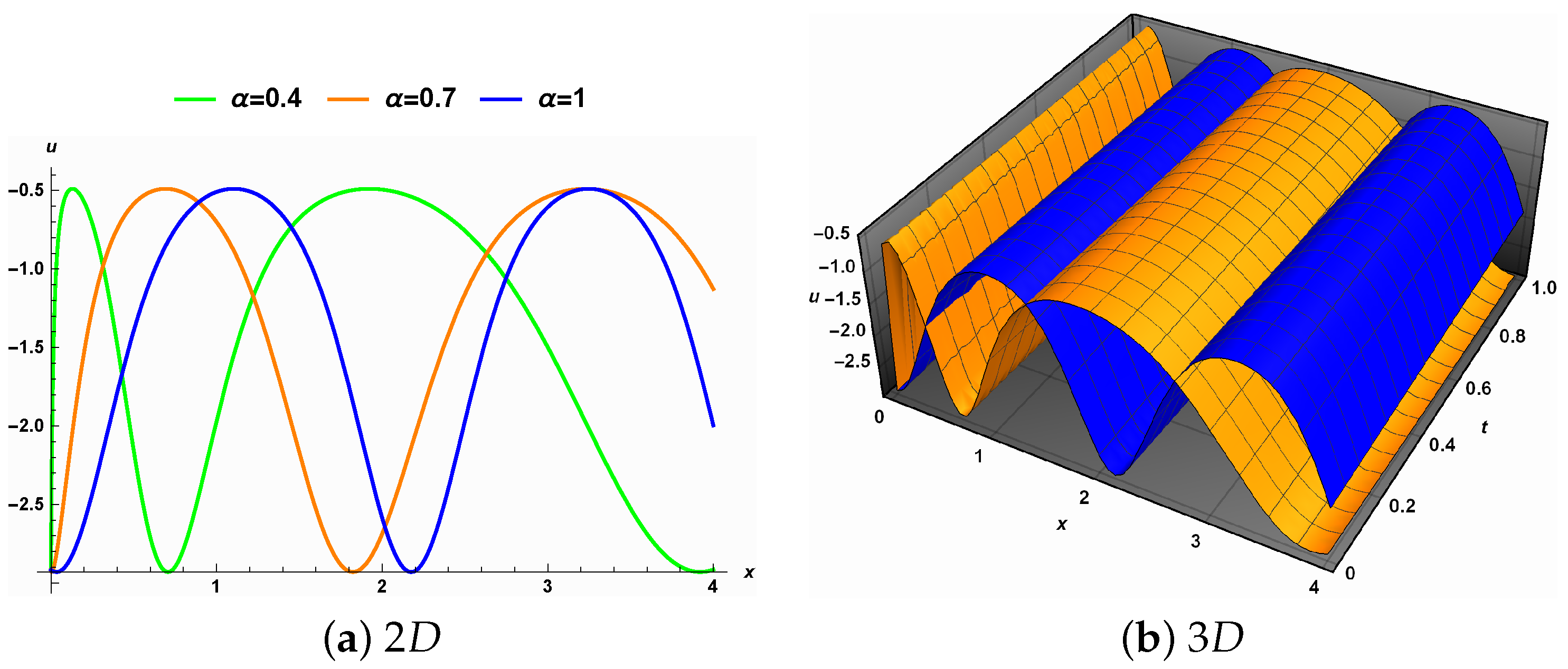
• (b) The fractional order effect. Figure 5a illustrates the impact of the fractional order $\alpha$ in the deterministic status $(\sigma =0)$ through the deviations surrounding the the blue line. The wavelength of Solution (27) increases as the fractional order $\alpha$ moves away from 1, while the amplitude remains almost the same. The corresponding 3D representation of the solution is shown in Figure 5b.
  

  Figure 5. The effect of the fractional order derivative $\alpha$ on Solution (27) in the deterministic case.
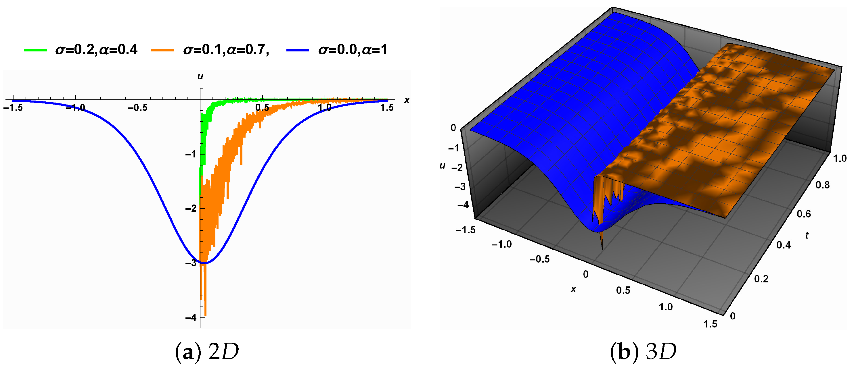
• (c) The combined influence. Figure 6a shows that the amplitude and wavelength of Solution (27) increase when both the noise intensity and the fractional order move away from 0 and 1, respectively. The surface characterized by Solution (27) that is smooth for $\sigma =0,\gamma \to 1$ becomes a rough surface, as shown in Figure 6b.
  

  Figure 6. The combined effect of noise intensity and fractional order derivative on Solution (27).

This discussion can be summarized by the following lemma.

Lemma 3.

For Solution (19), the further σ is from 0, the noisier the curve. On the other hand, the further σ is from 1 and the closer it is to 0, the more the curve loses its periodicity by gradually increasing the wavelength.

• 2. Deviation from the soliton solution

For the values $\beta =1$ and $\gamma =2$, we choose $s=0$. Hence, Solution (23), becomes

$$U(x,y,x,t)=\left[-3{\sec \mathrm{h}}^2\left(\frac{0.7071067810}{\alpha }(b_1{x}^{\alpha }+b_2{y}^{\alpha }+b_3{z}^{\alpha }-ct)\right)\right]e^{\sigma \mathbb{G}\left(t\right)-\frac{1}{2}{\sigma }^{2}t}.$$

(28)

• (a) The noise effect. Figure 7a illustrates the 2D representation of Solution (28) for different noise intensity values when the fractional order $\alpha =1$. The wave height increases while the width remains almost the same as the noise intensity increases. Figure 7b shows the surface characterized by this solution, which loses its smoothness as the noise intensity increases. Further, as the noise intensity increases, the surface flattens.
  

  Figure 7. The effect of noise intensity on Solution (28) when the fractional order $\alpha$ is one.
• (b) The fractional order effect. Figure 8a shows the effect of the fractional order derivative $\alpha$ on Solution (28) when $\sigma =0$. As the fractional order moves away from 1, Solution (28) gradually loses part of its wave structure and smoothness. The 3D representation is shown in Figure 8b.
  

  Figure 8. The effect of the fractional order derivative $\alpha$ on Solution (28) in the deterministic case.
• (c) The combined influence. Figure 9a shows the combined effect of $\sigma$ and $\alpha$. Solution (28) loses part of its wave structure and smoothness. The same conclusion can be drawn for the corresponding 3D representation and the surface gradually becomes rougher, as shown in Figure 9b.
  

  Figure 9. The combined effect of noise intensity and fractional order derivative on Solution (28).

The following lemma summarizes this discussion.

Lemma 4.

For solution (23), the further σ is from 0, the noisier the curve. On the other hand, the further σ is from 1 and the closer it is to 0, the more the curve loses part of its structure and gradually loses its smoothness.

6. Conclusions

The current work aimed to explore the impact of spatial fractional derivatives and the multiplicative Wiener process on the analytical solutions for (3+1)-dimensional fractional stochastic equations for fluids with gas bubbles. The bifurcation of the solutions was studied and some new solutions were introduced. These solutions were also new to the deterministic version of Equation (1), with derivatives that were either integers or fractions. Additionally, they were new for the stochastic integer-order derivative version of Equation (1). We concentrated on only forming real solutions for particular regions, which are called regions of real propagation. This type of solution is significant because it is applicable to real-world scenarios. On the other hand, the obtained exact solutions were significant because of their ability to describe diverse crucial challenges in weakly nonlinear waves propagating in liquids with gas bubbles, which are described by the fractional stochastic Equation (1). We graphically illustrated the individual impact of noise intensity and fractional order derivative, as well as the combined effect of both. These effects could be clearly observed in the amplitude, wavelength, and periodicity of the solutions. Furthermore, the smooth surface represented by the solution in the deterministic case became rough due to the noise term and lost its periodicity due to the fractional-order term.

References

- Lax, P.D. Integrals of nonlinear equations of evolution and solitary waves. Commun. Pure Appl. Math. 1968, 21, 467–490. [Google Scholar] [CrossRef]
- Ma, W.X.; Strampp, W. An explicit symmetry constraint for the Lax pairs and the adjoint Lax pairs of AKNS systems. Phys. Lett. A 1994, 185, 277–286. [Google Scholar] [CrossRef]
- Ramm, A. Inverse scattering with non-over-determined data. In Proceedings of the 2016 IEEE International Conference on Mathematical Methods in Electromagnetic Theory (MMET), Lviv, Ukraine, 5–7 July 2016; pp. 85–88. [Google Scholar]
- Hirota, R. Exact solution of the Korteweg—De Vries equation for multiple collisions of solitons. Phys. Rev. Lett. 1971, 27, 1192. [Google Scholar] [CrossRef]
- Radha, R.; Lakshmanan, M. Singularity analysis and localized coherent structures in (2+1)-dimensional generalized Korteweg–de Vries equations. J. Math. Phys. 1994, 35, 4746–4756. [Google Scholar] [CrossRef]
- Wazwaz, A.M. Two new integrable fourth-order nonlinear equations: Multiple soliton solutions and multiple complex soliton solutions. Nonlinear Dyn. 2018, 94, 2655–2663. [Google Scholar] [CrossRef]
- He, J.H. Variational iteration method—Some recent results and new interpretations. J. Comput. Appl. Math. 2007, 207, 3–17. [Google Scholar] [CrossRef]
- Schmid, R. Infinite Dimentional Lie Groups with Applications to Mathematical Physics. J. Geom. Symmetry Phys. 2004, 1, 54–120. [Google Scholar]
- Khalique, C.M.; Biswas, A. Optical solitons with power law nonlinearity using Lie group analysis. Phys. Lett. A 2009, 373, 2047–2049. [Google Scholar] [CrossRef]
- Fan, E.; Zhang, H. A note on the homogeneous balance method. Phys. Lett. A 1998, 246, 403–406. [Google Scholar] [CrossRef]
- Wang, M.; Zhou, Y.; Li, Z. Application of a homogeneous balance method to exact solutions of nonlinear equations in mathematical physics. Phys. Lett. A 1996, 216, 67–75. [Google Scholar] [CrossRef]
- Feng, Z. The first-integral method to study the Burgers–Korteweg–de Vries equation. J. Phys. Math. Gen. 2002, 35, 343. [Google Scholar] [CrossRef]
- Taghizadeh, N.; Mirzazadeh, M.; Farahrooz, F. Exact solutions of the nonlinear Schrödinger equation by the first integral method. J. Math. Anal. Appl. 2011, 374, 549–553. [Google Scholar] [CrossRef]
- Elbrolosy, M.; Elmandouh, A. Dynamical behaviour of nondissipative double dispersive microstrain wave in the microstructured solids. Eur. Phys. J. Plus 2021, 136, 1–20. [Google Scholar] [CrossRef]
- Elbrolosy, M.; Elmandouh, A. Dynamical behaviour of conformable time-fractional coupled Konno-Oono equation in magnetic field. Math. Probl. Eng. 2022, 2022, 3157217. [Google Scholar] [CrossRef]
- Elmandouh, A.A.; Elbrolosy, M.E. New traveling wave solutions for Gilson–Pickering equation in plasma via bifurcation analysis and direct method. Math. Methods Appl. Sci. 2022, 1–19. [Google Scholar] [CrossRef]
- Elmandouh, A.; Elbrolosy, M. Integrability, Variational Principle, Bifurcation, and New Wave Solutions for the Ivancevic Option Pricing Model. J. Math. 2022, 2, 3. [Google Scholar] [CrossRef]
- Siddique, I.; Mehdi, K.B.; Jaradat, M.M.; Zafar, A.; Elbrolosy, M.E.; Elmandouh, A.A.; Sallah, M. Bifurcation of some new traveling wave solutions for the time–space M-fractional MEW equation via three altered methods. Results Phys. 2022, 41, 105896. [Google Scholar] [CrossRef]
- Arnold, L. Trends and open problems in the theory of random dynamical systems. In Probability towards 2000; Springer: Berlin/Heidelberg, Germany, 1998; pp. 34–46. [Google Scholar]
- Weinan, E.; Li, X.; Vanden-Eijnden, E. Some recent progress in multiscale modeling. Multiscale Model. Simul. 2004, 39, 3–21. [Google Scholar]
- Mohammed, W.W.; Iqbal, N.; Botmart, T. Additive noise effects on the stabilization of fractional-space diffusion equation solutions. Mathematics 2022, 10, 130. [Google Scholar] [CrossRef]
- Mohammed, W.W.; Alshammari, M.; Cesarano, C.; Albadrani, S.; El-Morshedy, M. Brownian Motion Effects on the Stabilization of Stochastic Solutions to Fractional Diffusion Equations with Polynomials. Mathematics 2022, 10, 1458. [Google Scholar] [CrossRef]
- Elmandouh, A.; Fadhal, E. Bifurcation of Exact Solutions for the Space-Fractional Stochastic Modified Benjamin–Bona–Mahony Equation. Fractal Fract. 2022, 6, 718. [Google Scholar] [CrossRef]
- Van Wijngaarden, L. On the equations of motion for mixtures of liquid and gas bubbles. J. Fluid Mech. 1968, 33, 465–474. [Google Scholar] [CrossRef]
- Plesset, M.S.; Sadhal, S.S. On the stability of gas bubbles in liquid-gas solutions. In Mechanics and Physics of Bubbles in Liquids; Springer: Berlin/Heidelberg, Germany, 1982; pp. 133–141. [Google Scholar]
- Deng, G.F.; Gao, Y.T. Integrability, solitons, periodic and travelling waves of a generalized (3+ 1)-dimensional variable-coefficient nonlinear-wave equation in liquid with gas bubbles. Eur. Phys. J. Plus 2017, 132, 1–17. [Google Scholar] [CrossRef]
- Tu, J.M.; Tian, S.F.; Xu, M.J.; Song, X.Q.; Zhang, T.T. Bäcklund transformation, infinite conservation laws and periodic wave solutions of a generalized (3+ 1)-dimensional nonlinear wave in liquid with gas bubbles. Nonlinear Dyn. 2016, 83, 1199–1215. [Google Scholar] [CrossRef]
- Kudryashov, N.A.; Sinelshchikov, D.I. Equation for the three-dimensional nonlinear waves in liquid with gas bubbles. Phys. Scr. 2012, 85, 025402. [Google Scholar] [CrossRef]
- Ablowitz, M.J.; Segur, H. On the evolution of packets of water waves. J. Fluid Mech. 1979, 92, 691–715. [Google Scholar] [CrossRef]
- Ma, W.X.; Zhu, Z. Solving the (3+1)-dimensional generalized KP and BKP equations by the multiple exp-function algorithm. Appl. Math. Comput. 2012, 218, 11871–11879. [Google Scholar] [CrossRef]
- Ma, W.X.; Xia, T. Pfaffianized systems for a generalized Kadomtsev–Petviashvili equation. Phys. Scr. 2013, 87, 055003. [Google Scholar] [CrossRef]
- Alexander, J.; Pego, R.; Sachs, R. On the transverse instability of solitary waves in the Kadomtsev-Petviashvili equation. Phys. Lett. A 1997, 226, 187–192. [Google Scholar] [CrossRef]
- Yadav, S.; Arora, R. Lie symmetry analysis, optimal system and invariant solutions of (3+ 1)-dimensional nonlinear wave equation in liquid with gas bubbles. Eur. Phys. J. Plus 2021, 136, 1–25. [Google Scholar] [CrossRef]
- Khalil, R.; Al Horani, M.; Yousef, A.; Sababheh, M. A new definition of fractional derivative. J. Comput. Appl. Math. 2014, 264, 65–70. [Google Scholar] [CrossRef]
- Platen, E.; Bruti-Liberati, N. Numerical Solution of Stochastic Differential Equations with Jumps in Finance; Springer Science & Business Media: Cham, Switzerland, 2010; Volume 64. [Google Scholar]
- Kumar, S.; Hamid, I.; Abdou, M. Specific wave profiles and closed-form soliton solutions for generalized nonlinear wave equation in (3+1)-dimensions with gas bubbles in hydrodynamics and fluids. J. Ocean. Eng. Sci. 2021; in press. [Google Scholar] [CrossRef]
- Nemytskii, V.; Stepanov, V. Qualitative Theory of Differential Equations; Courier Dover Publications: New York, NY, USA, 1989; Volume 22. [Google Scholar]