Analytical and Numerical Study of Nonlinear Variable-Order Time Fractional Reaction-Diffusion Coupled Equations Arising in Biological and Chemical Processes

Abstract

In this article, we analyze a category of time-fractional variable-order reaction-diffusion equations coupled in the Caputo sense that are created with the modeling of complicated biological and chemical processes. Furthermore, it is shown that the solutions exist and are unique, and then the system is subjected to the Ulam-Hyers stability, which confirms the model’s reliability and robustness. An advanced solution method based on shifted second-kind Airfoil polynomials is proposed for the numerical solution, where the polynomials are used to derive an operational matrix for variable-order fractional derivatives that is then applied to the original system using the collocation method to convert it into an equivalent set of algebraic equations. The system created is solved in order to obtain very precise approximations of the unknown functions. The proposed method is illustrated through several numerical experiments that not only show its accuracy but also its efficiency. The results obtained prove that the method is superior to the currently existing numerical techniques for fractional reaction-diffusion systems.

1. Introduction

The fractional calculus is an area of mathematical analysis which, in a sense, opens up a world of new possibilities since it introduces the concept of differentiation and integration of any order, including non-integer ones, as its fundamental operations. A detailed account of the subject can be found in [1,2]. Equations that incorporate derivatives of fractional order, known as fractional differential equations (FDEs), have emerged as a central topic in contemporary research, as they provide a powerful framework for modeling physical and biological systems with memory and hereditary properties that cannot be satisfactorily represented by classical integer-order models. In the last years, the applications of fractional differential equations (FDEs) have been a hot topic mainly because of their capability of portraying phenomena with memory and hereditary effects that conventional integer-order models cannot represent well. (FDEs) have found many applications in practically all areas of science and engineering, including but not limited to physics, biology, engineering, economics, and finance. They are, for instance, implemented in the simulation of diverse phenomena such as heat conduction in materials with different properties, unusual diffusion in media with pores, and fluid characterized by both viscosity and elasticity. The use of nonlocal operators in fractional models makes them more physically accurate descriptions of nature than their integer-order counterparts [3,4,5]. In the literature, multiple definitions of fractional derivatives have been proposed, among which the ones based on Riemann–Liouville, Caputo, Riesz, Hadamard, and Grünwald–Letnikov are particularly noteworthy. Among these, the Caputo derivative is widely employed in physical and engineering problems because it enables the specification of standard initial conditions involving integer-order derivatives. Moreover, the classical notion of a constant fractional order has been extended to the notion of variable-order (VO) derivatives, this can only happen in a maximum-order derivative, in which differentiation order can function from an upper bound through the spatial and/or temporal derivatives. This idea is very helpful in simulating processes that have a memory effect differing with position or time. For instance, (VO) derivatives have been used in the case of diffusion processes in heterogeneous media, signal processing, and viscoelastic materials [6,7,8]. Their adaptability renders them an essential instrument for revealing the intricacies of dynamics that vary with both the scale and the environment, see for example [9].

In that context, fractional reaction-diffusion equations are considered as a major type of models owing to their broad use in natural sciences. The main idea behind reaction-diffusion systems is to describe the balance of diffusion, which is the main factor for the spatial distribution of substances, and the nonlinear reactions, which control the local dynamics. The behavior of these systems ranges from pattern formation and wave propagation to other complex behaviors, and hence they are considered as indispensable tools for studying various problems in chemistry, biology, and ecology. The classic examples of this category include the Gray-Scott model, Schnakenberg system, and the Brusselator model, which are commonly used to examine the phenomenon of pattern formation in chemical reactions as well as the dynamics of biological populations. Extending such systems to the fractional and variable-order settings introduces memory and anomalous transport effects, offering deeper insights into real-world processes where standard reaction-diffusion equations fall short [10,11].

In the present work, we investigate a variable-order time fractional reaction–diffusion system of coupled equations:

$$\begin{array}{cc}\hfill D_{\varsigma }^{{\alpha }_1(\varrho ,\varsigma )}\mathcal{U}(\varrho ,\varsigma )& =a_1{\mathcal{U}}_{\varrho \varrho }+p_1\mathcal{U}+q_1\mathcal{V}+s_1{\mathcal{U}}^2\mathcal{V}+n_1\mathcal{U}\mathcal{V}+m_1\mathcal{U}{\mathcal{V}}^2\hfill \\ \hfill & +{\kappa }_1+{\mathcal{F}}_1(\varrho ,\varsigma ),\varrho \in \mathrm{\Omega },\varsigma >0.\hfill \\ \hfill D_{\varsigma }^{{\alpha }_2(\varrho ,\varsigma )}\mathcal{V}(\varrho ,\varsigma )& =a_2{\mathcal{V}}_{\varrho \varrho }+p_2\mathcal{U}+q_2\mathcal{V}+s_2{\mathcal{U}}^2\mathcal{V}+n_2\mathcal{U}\mathcal{V}+m_2\mathcal{U}{\mathcal{V}}^2\hfill \\ \hfill & +{\kappa }_2+{\mathcal{F}}_2(\varrho ,\varsigma ),\varrho \in \mathrm{\Omega },\varsigma >0.\hfill \end{array}$$

(1)

The associated initial conditions (ICs) are:

$$\begin{array}{c}\hfill \mathcal{U}(\varrho ,0)={\mathcal{U}}_0\left(\varrho \right).\end{array}$$

(2)

$$\begin{array}{c}\hfill \mathcal{V}(\varrho ,0)={\mathcal{V}}_0\left(\varrho \right).\end{array}$$

(3)

In the manner thus ordered, the boundary conditions (BCs) are listed:

• Type 1:

  $$\begin{array}{cc}\hfill \mathcal{U}({\varrho }_0,\varsigma )& ={\epsilon }_0\left(\varsigma \right),\mathcal{U}({\varrho }_N,\varsigma )={\delta }_0\left(\varsigma \right),\varsigma >0.\hfill \\ \hfill \mathcal{V}({\varrho }_0,\varsigma )& ={\epsilon }_1\left(\varsigma \right),\mathcal{V}({\varrho }_N,\varsigma )={\delta }_1\left(\varsigma \right),\varsigma >0.\hfill \end{array}$$

  (4)
• Type 2:

  $$\begin{array}{cc}\hfill {\mathcal{U}}_{\varrho }({\varrho }_0,\varsigma )& ={\epsilon }_0\left(\varsigma \right),\mathcal{U}({\varrho }_N,\varsigma )={\delta }_0\left(\varsigma \right),\varsigma >0.\hfill \\ \hfill {\mathcal{V}}_{\varrho }({\varrho }_0,\varsigma )& ={\epsilon }_1\left(\varsigma \right),\mathcal{V}({\varrho }_N,\varsigma )={\delta }_1\left(\varsigma \right),\varsigma >0.\hfill \end{array}$$

  (5)
• Type 3:

  $$\begin{array}{cc}\hfill {\mathcal{U}}_{\varrho }({\varrho }_0,\varsigma )& ={\epsilon }_0\left(\varsigma \right),{\mathcal{U}}_{\varrho }({\varrho }_N,\varsigma )={\delta }_0\left(\varsigma \right),\varsigma >0.\hfill \\ \hfill {\mathcal{V}}_{\varrho }({\varrho }_0,\varsigma )& ={\epsilon }_1\left(\varsigma \right),{\mathcal{V}}_{\varrho }({\varrho }_N,\varsigma )={\delta }_1\left(\varsigma \right),\varsigma >0.\hfill \end{array}$$

  (6)

In the Equation (1), both $\mathcal{U}(\varrho ,\varsigma )$ and $\mathcal{V}(\varrho ,\varsigma )$ are the functions of two independent variables, which characterize the dynamics when $0<{\alpha }_1<{\alpha }_2<1$, and for each $j=1,2$, $a_j,p_j,q_j,s_j,n_j,m_j$ and ${\kappa }_j$ are real constants that have some physical interpretation.

Here, $a_j$ ($j=1,2$) denote the diffusion coefficients of the interacting variables $\mathcal{U}$ and $\mathcal{V}$. The parameters $p_j$ and $q_j$ represent the linear reaction and interaction coefficients, while $s_j$, $n_j$, and $m_j$ correspond to nonlinear interaction terms describing higher-order coupling effects between $\mathcal{U}$ and $\mathcal{V}$. The constants ${\kappa }_j$ represent constant source terms. All parameters are assumed to be real constants. The source terms are represented by ${\mathcal{F}}_1$ and ${\mathcal{F}}_2$, while $\Omega =[{\varrho }_0,{\varrho }_N]$ denotes the spatial domain that is further subdivided into M smaller subintervals. Each interval has the width of $d\varrho ={\displaystyle \frac{{\varrho }_N-{\varrho }_0}{M}}$. The system is then coupled with the corresponding initial and boundary conditions to make it complete. Such equations arise naturally in the modeling of biological and chemical processes, where nonlinear interactions and spatial heterogeneity play essential roles. The inclusion of (VO) fractional derivatives further enhances the model by accounting for space and time dependent memory effects.

The main goal of this research paper is to develop a complete numerical framework that uses the second kind of shifted Airfoil collocation method along with the operational matrix technique to obtain approximate solutions for the system under study. The operational matrices stem from the shifted second-kind Airfoil polynomials, and the appropriate collocation points are determined; therefore, the governing system is transformed into a system of algebraic equations whose capable solution yields very precise numerical approximations. Even though the orthogonality of these polynomials reduces the computational cost greatly, it doesn’t compromise the accuracy. The method’s validity is supported by comparisons with existing analytical or numerical results. The ongoing research involves the use of fractal-fractional operators, transform-based techniques, and polynomial-based operational matrices in other fractional system contexts [12,13].

For the model to have a valid mathematical interpretation and to be applied to the area of physics, one important part of the analysis is to prove that the corresponding solutions exist and are unique, which means that for certain starting conditions, there is only one solution that will change in a consistent way through time.

In addition, we explore the stability of Ulam-Hyers that guarantees the proximity of approximate solutions, for instance, the one achieved numerically, to the exact solution if the perturbation is small. This characteristic is very important in affirming the dependability of computational techniques, particularly in the case of modeling sensitive biological interactions where a slight change can cause a totally different outcome [14,15].

Many studies are available in the literature that would be directly relevant to this work. For example, ref. [16] explored numerical techniques based on the fractal–fractional derivative operator. In [17], a Laguerre wavelet method was proposed to investigate the motion of a fractional predator–prey population system. The numerical analysis of a fractional-order tumor–immune–vitamin interaction model was carried out in [18]. Besides, ref. [19] developed a new operational matrix technique based on generalized polynomials to derive numerical solutions of the variable-order nonlinear Klein–Gordon equation. Similarly, ref. [20] introduced a numerical method based on generalized Chebyshev polynomials for the solution of nonlinear variable-order fractional partial differential equations (VOFPDEs). Moreover, ref. [21] used the generalized Bernstein polynomial method for the numerical solution of the variable-order space–time fractional telegraph equation.

The essential innovations and unique aspects distinguishing this study are enumerated below:

• This research offers a pioneering definition and numerical appraisal of the coupled systems of reaction-diffusion with a different fractional order, which incorporates nonlinear interaction terms and space–time dependent memory effects within a unified fractional framework. This generalization extends the classical integer-order and fixed-order reaction–diffusion equations discussed in [22,23], enabling a more realistic description of complex physical and biological processes.
• Although several recent contributions such as [24,25] have explored fractional or variable-order models, most focus on single equations or systems with constant fractional orders. In contrast, the present work develops a coupled nonlinear system involving two distinct variable fractional orders, $0<{\alpha }_1(x,t)<{\alpha }_2(x,t)<1$, thereby extending variable-order fractional dynamics to multi-component diffusion–reaction phenomena.
• One of the most significant computational breakthroughs is the development of a hybrid numerical algorithm created by combining the method of second shifted collocation for airfoil and the operational matrix method. Unlike classical transform or polynomial-based techniques [26,27], the proposed strategy transforms the fractional coupled system into a low-dimensional algebraic system with enhanced accuracy, numerical stability, and computational efficiency.
• In contrast to existing methods employing Chebyshev, Bernstein, or wavelet-based operational matrices [28,29], the proposed scheme utilizes the orthogonality and smoothness of shifted airfoil polynomials, which ensures rapid convergence, minimal truncation error, and improved stability when applied to nonlinear coupled systems of variable fractional order.
• The paper from an analytical perspective has established the proof for the existence and uniqueness of the solution for the internal (VO) fractional coupled system, thereby assuring mathematical and at the same time, physical consistency. Theoretical considerations, which are sometimes neglected in numerical simulations, ref. [30] have implicitly affirmed the strength of the model that has been developed.
• Moreover, one attempt is being made at reviewing the Ulam-Hyers stability of the new-variable fractional-order system. This stability analysis assures that the approximate numerical solutions will not deviate much from the exact solutions even if small perturbations occur, thus establishing a crucial connection between theoretical and computational reliability. As per our knowledge, no such stability analysis for coupled variable-order reaction–diffusion systems has been published earlier [31,32]. In addition to exploring the stabilities of the presented new variable-order systems, the research emphasizes searching for the Ulam-Hyers stability aspect. This stability analysis assures that the approximate numerical solutions will not deviate much from the exact solutions even if small perturbations occur, thus establishing a crucial connection between theoretical and computational reliability. As per our knowledge, no such stability analysis for coupled variable-order reaction–diffusion systems has been published earlier [33,34,35].
• The suggested hybrid operational matrix utilizing shifted airfoil polynomials shows superior numerical efficiency over earlier polynomial methods developed for generalized Laguerre or Gegenbauer bases [36,37]. The method is versatile and can be easily modified to apply to other nonlinear fractional systems with multi-term or mixed fractional operators.
• The described method is able to handle various kinds of that boundary conditions (Dirichlet, mixed, and Neumann) at the same time, thus it is more versatile than the regular fixed-order numerical schemes [38,39]. The advantage of this method is that it can be applied in many boundary-controlled diffusion–reaction processes.
• The research additionally offers a convergence and error analysis of an all-encompassing nature, which is a showcase of the effectiveness of the suggested method in connection with mesh refinement and variable fractional order. This type of quantitative error evaluation is seldom mentioned in earlier fractional numerical models [40].
• Ultimately, the theoretical progress and numerical method are verified by means of extensive comparative simulations with published data [22,24]. The visual representations corroborate the precision, robustness, and physical significance of the suggested method and provide new perspectives on the fractional modeling of nonlinear diffusion-reaction systems.

The paper is structured in a very clear way, whereby seven sections are presented in total. The first section provides a brief introduction to the main ideas, namely the Riemann-Liouville fractional integral, Caputo-type fractional derivatives, and second-kind airfoil polynomials with their basic properties. The next section covers the operational matrix derivation for variable-order derivatives. In the following section, the author presents and justifies the existence-uniqueness-stability properties of the solution through an extensive discussion on the subject. Section 5 gives an in-depth treatment of the numerical method that has been proposed. Numerical experiments are reported in Section 6 aimed at demonstrating the potency of the proposed method, while Section 7 wraps up the paper with a summary of its key findings.

2. Preliminaries

The effectiveness of our numerical results is greatly strengthened through a fundamental comprehension of fractional calculus and its associated analytical techniques.

Definition 1. 

For a function $h(\varrho ,\varsigma )$ and variable fractional order $\beta (\varrho ,\varsigma )\in (0,1]$, the integral Riemann–Caputo is defined conventionally as [41]

$${\displaystyle I_{\varsigma }^{\beta (\varrho ,\varsigma )}h(\varrho ,\varsigma )={\displaystyle \frac{1}{\mathrm{\Gamma }\left(\beta \right(\varrho ,\varsigma \left)\right)}}{\int }_0^{\varsigma }{(\varsigma -s)}^{\beta (\varrho ,\varsigma )-1}h(\varrho ,s)ds.}$$

Definition 2. 

For a given function $h(\varrho ,\varsigma )$, the Caputo fractional derivative of variable order $\beta (\varrho ,\varsigma )$ is mathematically expressed as [42]

$$D_{\varsigma }^{\beta (\varrho ,\varsigma )}h(\varrho ,\varsigma )=\left\{\begin{array}{cc}{\displaystyle \frac{1}{\mathrm{\Gamma }\left(q-\beta (\varrho ,\varsigma )\right)}{\int }_0^{\varsigma }{(\varsigma -\rho )}^{q-\beta (\varrho ,\varsigma )-1}\frac{{\partial }^{q}h(\varrho ,\rho )}{\partial {\rho }^q}d\rho ,}\hfill & q-1<\beta (\varrho ,\varsigma )<q,q\in \mathbb{N},\hfill \\ {\displaystyle \frac{{\partial }^{q}h(\varrho ,\varsigma )}{\partial {\varsigma }^q},}\hfill & \beta (\varrho ,\varsigma )=q.\hfill \end{array}\right.$$

The operator $D_{\varsigma }^{\beta (\varrho ,\varsigma )}$ has the following properties

$$D_{\varsigma }^{\beta (\varrho ,\varsigma )}(\lambda h(\varrho ,\varsigma )+\mu g(\varrho ,\varsigma ))=\lambda D_{\varsigma }^{\beta (\varrho ,\varsigma )}h(\varrho ,\varsigma )+\mu D_{\varsigma }^{\beta (\varrho ,\varsigma )}g(\varrho ,\varsigma ),$$

(7)

$D_{\varsigma }^{\beta (\varrho ,\varsigma )}C=0$, C is a constant and

$$D_{\varsigma }^{\beta (\varrho ,\varsigma )}{\varsigma }^{\vartheta }=\left\{\begin{array}{cc}0,\hfill & \vartheta \in 0,1,2,\dots ,q-1,\hfill \\ {\displaystyle {\displaystyle \frac{\mathrm{\Gamma }(\vartheta +1)}{\mathrm{\Gamma }(\vartheta +1-\beta (\varrho ,\varsigma \left)\right)}}{\varsigma }^{\vartheta -\beta (\varrho ,\varsigma )},}\hfill & \mathrm{otherwise},\hfill \end{array}\right.$$

(8)

when the derivative order is between $q-1$ and q, and where the letter $\mathrm{\Gamma }(·)$ denotes the Gamma function.

Definition 3. 

The two-parameter Mittag–Leffler function defined for a real variable h and with positive parameters i and j can be expressed as [43]

$$E_{i,j}\left(h\right)=1+{\displaystyle \frac{h}{\mathrm{\Gamma }(i+j)}}+{\displaystyle \frac{h^2}{\mathrm{\Gamma }(2i+j)}}+{\displaystyle \frac{h^3}{\mathrm{\Gamma }(3i+j)}}+\dots$$

2.1. Airfoil Polynomials and Their Shifted Forms

In this subsection, the second kind of Airfoil polynomials and their essential characteristics are examined. They are constructed through the recursive formula given below [44]

$${\mathbb{A}}_{n+1}\left(l\right)=2l{\mathbb{A}}_n\left(l\right)-{\mathbb{A}}_{n-1}\left(l\right).n=1,2,3,\dots ,$$

(9)

with the initial values

$${\mathbb{A}}_0\left(l\right)=1,{\mathbb{A}}_1\left(l\right)=2l+1.$$

The second kind of airfoil polynomial ${\mathbb{A}}_n\left(l\right)$ can be written explicitly in the following expanded form

$${\mathbb{A}}_n\left(l\right)={\displaystyle \frac{1}{2^n}}\sum _{j=0}^n{(-1)}^j\left({\displaystyle \genfrac{}{}{0pt}{}{2n+1}{2j+1}}\right){(1-l)}^j{(1+l)}^{n-j}.n=0,1,2,3,\dots$$

(10)

The polynomials in the family $\mathbb{A}\left(l\right)$ are orthogonal over the interval $[-1,1]$ with the weight function $\omega \left(l\right)=\sqrt{{\displaystyle \frac{1-l}{1+l}}}$. This weight function is defined as

$${\displaystyle {\int }_{-1}^1{\mathbb{A}}_m\left(l\right){\mathbb{A}}_n\left(l\right)\omega \left(l\right)dl=\left\{\begin{array}{cc}\pi ,\hfill & m=n,\hfill \\ 0,\hfill & m\ne n.\hfill \end{array}\right.}$$

(11)

It should be noted that the weight function

$$\omega \left(l\right)=\sqrt{{\displaystyle \frac{1-l}{1+l}}}$$

has integrable singularities at the endpoints $l=\pm 1$. However, the orthogonality relation is understood in the sense of improper integrals over the open interval $(-1,1)$, for which the integral remains finite. Shifted polynomials need to be used on the interval $[0,1]$. Hence, let’s start by defining these polynomials,

$${\mathbb{A}}_n^{\ast }\left(l\right)={\mathbb{A}}_n(2l-1).$$

(12)

By using the aforementioned transformation in Equation (9), the recurrence becomes

$${\Delta }^2{\mathbb{A}}_{n-1}^{\ast }\left(l\right)=2(2l-1){\mathbb{A}}_n^{\ast }\left(l\right).$$

(13)

Here, the operator $\Delta$ denotes the spatial Laplacian defined by

$${\displaystyle \Delta =\frac{{\partial }^2}{\partial {\varrho }^2}+\frac{{\partial }^2}{\partial {\varsigma }^2}.}$$

It is worth noting that the initial values of the shifted airfoil polynomials $A_n^{\ast }\left(l\right)$ are consistent with those of the original airfoil polynomials $A_n\left(l\right)$. Indeed, using the transformation defined in (12), $A_n^{\ast }\left(l\right)=A_n(2l-1)$, we have

$$A_n^{\ast }\left(0\right)=A_n(-1),A_n^{\ast }\left(1\right)=A_n\left(1\right);$$

which shows that the initial values of $A_n^{\ast }\left(l\right)$ directly follow from the corresponding initial values of $A_n\left(l\right)$. and explicit expansion form is provided as follows

$${\mathbb{A}}_n^{\ast }\left(l\right)=\sum _{j=0}^n{(-1)}^j\left({\displaystyle \genfrac{}{}{0pt}{}{2n+1}{2j+1}}\right){(1-l)}^j{l}^{n-j}.n=0,1,2,3,\dots$$

(14)

Equation (14) is obtained directly from Equation (10) by applying the variable transformation defined in Equation (12). Substituting $l=2l-1$ into Equation (11)and using $A_n^{\ast }\left(l\right)=A_n(2l-1)$, together with the chain rule for derivatives, the corresponding relation for the shifted airfoil polynomials is derived. This procedure leads straightforwardly to Equation (14).

Equation (14) can equivalently be expressed as

$${\mathbb{A}}_n^{\ast }\left(l\right)=\sum _{j=0}^n{(-1)}^{n-j}{\displaystyle \frac{2^{2j}\mathrm{\Gamma }(n+j+1)}{\mathrm{\Gamma }(n-j+1)\mathrm{\Gamma }(2j+1)}}{l}^j.n=0,1,2,3,\dots ,$$

(15)

with weight function ${\omega }^{\ast }(l)=\sqrt{{\displaystyle \frac{1-l}{l}}}$, acknowledging that the polynomials ${\mathbb{A}}_m^{\ast }$ for the distribution element are independent:

$${\displaystyle {\int }_0^1{\mathbb{A}}_m^{\ast }\left(l\right){\mathbb{A}}_n^{\ast }\left(l\right){\omega }^{\ast }(l)dl=\left\{\begin{array}{cc}{\displaystyle \frac{\pi }{2}},\hfill & m=n,\hfill \\ 0,\hfill & m\ne n.\hfill \end{array}\right.}$$

(16)

The weight function ${\omega }^{\ast }(l)$ associated with the shifted airfoil polynomials is obtained directly from the original weight function $\omega \left(l\right)$ through the variable transformation defined in Equation (12). Indeed, by letting $l=2l-1$ and $dl=2dl$, the orthogonality relation Equation (11) can be rewritten as

$${\int }_0^1{A}_m^{\ast }\left(l\right)A_n^{\ast }\left(l\right){\omega }^{\ast }(l)dl=0.m\ne n,$$

where the shifted weight function is given by

$${\omega }^{\ast }(l)=2\omega (2l-1).$$

This shows that the orthogonality property of the airfoil polynomials is preserved under the shifting transformation.

Since the shifted Airfoil polynomials $A_n^{\ast }\left(l\right)$ are defined on the interval $[0,1]$, we restrict the temporal domain to a finite interval $[0,T]$ and introduce the transformation

$$\tilde{\varsigma }={\displaystyle \frac{\varsigma }{T}},0\le \varsigma \le T,$$

so that $\tilde{\varsigma }\in [0,1]$.

We are now expanding our functions as

$$\mathcal{U}(\varrho ,\varsigma )\approx \sum _{m=0}^M\sum _{n=0}^N{a}_{mn}{\mathbb{A}}_m^{\ast }\left(\varrho \right)A_n^{\ast }\left(\varsigma \right).$$

(17)

Similarly for $\mathcal{V}(\varrho ,\varsigma )$

$$\mathcal{V}(\varrho ,\varsigma )\approx \sum _{m=0}^M\sum _{n=0}^N{b}_{mn}{\mathbb{A}}_m^{\ast }\left(\varrho \right)A_n^{\ast }\left(\varsigma \right).$$

(18)

2.2. Function Approximation

Assuming that the function $\mathcal{U}\left(l\right)$ is a member of $L^2\left([0,1]\right)$, it can be represented in the form of series through the second kind of shifted Airfoil polynomials, like this:

$$\mathcal{U}\left(l\right)=\sum _{J=0}^{\infty }{g}_j{\mathbb{A}}_j^{\ast }\left(l\right).$$

(19)

where the coefficients $g_j$ remain undetermined.

Generally, the formula portrayed in Equation (19) is computed using a limited series of the $(n+1)$ displaced second kind Airfoil polynomials, which are defined by

$$\mathcal{U}\left(l\right)\approx \sum _{j=0}^n{g}_j{\mathbb{A}}_j^{\ast }\left(l\right).$$

(20)

The Equation (20) can also be expressed in the matrix-vector form as:

$$\mathcal{U}\left(l\right)\approx G^T\mathrm{\Pi }\left(l\right),$$

(21)

We note that the truncation from the infinite series in Equation (19) to the finite series in Equation (20), and its corresponding matrix-vector form in Equation (21), introduces a standard spectral approximation error. This error depends on the smoothness of the function $\mathcal{U}$ or $\mathcal{V}$ and decreases rapidly as the number of basis polynomials n increases. Consequently, the truncated representation provides a highly accurate approximation for practical computations, as also confirmed by the numerical results presented in

Table 1. Error norms for $\mathcal{U}(\varrho ,\varsigma )$.

n	${{\mathit{L}}_2}^{\mathit{Set}1}$	${{\mathit{L}}_{\mathbf{\infty }}}^{\mathit{Set}1}$	${{\mathit{L}}_{\mathbf{2}}}^{\mathit{Set}2}$	${{\mathit{L}}_{\mathbf{\infty }}}^{\mathit{Set}2}$
3	$3.419\times {10}^{-3}$	$1.333\times {10}^{-3}$	$3.471\times {10}^{-3}$	$1.367\times {10}^{-3}$
5	$2.672\times {10}^{-5}$	$7.122\times {10}^{-6}$	$2.663\times {10}^{-5}$	$7.107\times {10}^{-6}$
7	$1.015\times {10}^{-7}$	$2.066\times {10}^{-8}$	$1.023\times {10}^{-7}$	$2.089\times {10}^{-8}$
9	$2.106\times {10}^{-10}$	$3.463\times {10}^{-11}$	$2.107\times {10}^{-10}$	$3.468\times {10}^{-11}$
11	$2.891\times {10}^{-13}$	$4.041\times {10}^{-14}$	$2.962\times {10}^{-13}$	$3.997\times {10}^{-14}$

and

Table 2. Error norms for $\mathcal{V}(\varrho ,\varsigma )$.

n	${{\mathit{L}}_2}^{\mathit{Set}1}$	${{\mathit{L}}_{\mathbf{\infty }}}^{\mathit{Set}1}$	${{\mathit{L}}_{\mathbf{2}}}^{\mathit{Set}2}$	${{\mathit{L}}_{\mathbf{\infty }}}^{\mathit{Set}2}$
3	$2.620\times {10}^{-3}$	$8.788\times {10}^{-4}$	$2.734\times {10}^{-3}$	$9.076\times {10}^{-4}$
5	$1.927\times {10}^{-5}$	$4.374\times {10}^{-6}$	$1.948\times {10}^{-5}$	$4.518\times {10}^{-6}$
7	$7.967\times {10}^{-8}$	$1.233\times {10}^{-8}$	$8.307\times {10}^{-8}$	$1.296\times {10}^{-8}$
9	$1.598\times {10}^{-10}$	$2.040\times {10}^{-11}$	$1.609\times {10}^{-10}$	$2.059\times {10}^{-11}$
11	$2.211\times {10}^{-13}$	$2.354\times {10}^{-14}$	$2.485\times {10}^{-13}$	$4.366\times {10}^{-14}$

.

Where

$$G^T=[g_0,g_1,g_2,\dots ,g_n],\mathrm{\Pi }\left(l\right)={[{\mathbb{A}}_0^{\ast }\left(l\right),{\mathbb{A}}_1^{\ast }\left(l\right),\dots ,{\mathbb{A}}_n^{\ast }\left(l\right)]}^T.$$

(22)

Here, $g_j$$(j=0,1,2,\dots ,c_n)$ denote the unknown coefficients, which can be determined using the following expression

$${\displaystyle g_j={\displaystyle \frac{2}{\pi }}{\int }_0^1\mathcal{U}\left(l\right){\mathbb{A}}_j^{\ast }{\omega }^{\ast }(l)dl.}$$

(23)

Now, As we are dealing with unknown functions $\mathcal{U}(\varrho ,\varsigma )$,and $\mathcal{V}(\varrho ,\varsigma )$. These are functions of $\varrho ,\varsigma$. To approximate these functions, we use Airfoil polynomials. For this, suppose an arbitrary function $\mathcal{U}(\varrho ,\varsigma )\in L^2(\left([0,1]\right)\times \left([0,1]\right))$, it can be described using a shifted airfoil polynomial given below

$$\mathcal{U}(\varrho ,\varsigma )=\sum _{j=0}^n\sum _{k=0}^m{v}_{jk}{\mathbb{A}}_j^{\ast }(\varrho ){\mathbb{A}}_k^{\ast }(\varsigma ).$$

(24)

where $v_{jk}$ are unknown time-dependent coefficients and is given by

$${\displaystyle v_{jk}={\displaystyle \frac{4}{{\pi }^2}}{\int }_0^1{\int }_0^1\mathcal{U}(\varrho ,\varsigma ){\mathbb{A}}_j^{\ast }(\varrho ){\mathbb{A}}_k^{\ast }(\varsigma ){\omega }^{\ast }(\varrho ){\omega }^{\ast }(\varsigma )d\varrho d\varsigma .}$$

(25)

The truncated series of Equation (24) can be given as below

$$\mathcal{U}(\varrho ,\varsigma )\approx \sum _{j=0}^n\sum _{k=0}^m{v}_{jk}{\mathbb{A}}_j^{\ast }\left(\varrho \right){\mathbb{A}}_k^{\ast }\left(\varsigma \right)={\mathrm{\Pi }}^T\left(\varrho \right)V\mathrm{\Pi }\left(\varsigma \right).$$

(26)

where

$$\begin{array}{c}\hfill \mathrm{\Pi }\left(\varrho \right)={[{\mathbb{A}}_0^{\ast }\left(\varrho \right),{\mathbb{A}}_1^{\ast }\left(\varrho \right),{\mathbb{A}}_2^{\ast }\left(\varrho \right),\dots ,{\mathbb{A}}_n^{\ast }\left(\varrho \right)]}^T,\\ \hfill \mathrm{and}\mathrm{\Pi }\left(\varsigma \right)={[{\mathbb{A}}_0^{\ast }\left(\varsigma \right),{\mathbb{A}}_1^{\ast }\left(\varsigma \right),{\mathbb{A}}_2^{\ast }\left(\varsigma \right),\dots ,{\mathbb{A}}_m^{\ast }\left(\varsigma \right)]}^T.\end{array}$$

(27)

$V\left(\varsigma \right)={\left(v_{jk}\right)}_{j,k=0}^{n,m}$.

Similarly for $\mathcal{V}(\varrho ,\varsigma )$, we have

$$\mathcal{V}(\varrho ,\varsigma )\approx \sum _{j=0}^n\sum _{k=0}^m{w}_{jk}{\mathbb{A}}_j^{\ast }\left(\varrho \right){\mathbb{A}}_k^{\ast }\left(\varsigma \right)={\mathrm{\Pi }}^T\left(\varrho \right)W\mathrm{\Pi }\left(\varsigma \right),$$

(28)

where $W\left(\varsigma \right)={\left(w_{jk}\right)}_{j,k=0}^{n,m}.$

Theorem 1. 

The derivative of the translated or shifted airfoil vector $\mathrm{\Pi }\left(\varrho \right)$ is then presented

$${\displaystyle \frac{d^1\mathrm{\Pi }\left(\varrho \right)}{d\varrho }}=M^{\left(1\right)}\mathrm{\Pi }\left(\varrho \right).$$

(29)

In this system, $M^{\left(1\right)}={\left(m_{ij}\right)}_{(n+1)\times (n+1)}$ represents the operational matrix which refers to the first-order derivative and satisfies

$$m_{ij}=\left\{\begin{array}{cc}2(j-i),\hfill & wheni>jand(i+j)iseven,\hfill \\ 2(i+j+1),\hfill & wheni>jand(i+j)isodd,\hfill \\ 0,\hfill & otherwise.\hfill \end{array}\right.$$

(30)

Thus, the 2nd and 3rd order definitions of vector $\mathrm{\Pi }\left(\varrho \right)$ are as

$${\displaystyle \frac{d^2\mathrm{\Pi }\left(\varrho \right)}{d{\varrho }^2}}=M^{{\left(1\right)}^2}\mathrm{\Pi }\left(\varrho \right)=M^{\left(2\right)}\mathrm{\Pi }\left(\varrho \right),$$

(31)

and

$${\displaystyle \frac{d^3\mathrm{\Pi }\left(\varrho \right)}{d{\varrho }^3}}=M^{{\left(1\right)}^3}\mathrm{\Pi }\left(\varrho \right)=M^{\left(3\right)}\mathrm{\Pi }\left(\varrho \right).$$

(32)

From Equations (31) and (32), we have the kth order derivatives of vector $\mathrm{\Pi }\left(\varrho \right)$ can we written as

$${\displaystyle \frac{d^k\mathrm{\Pi }\left(\varrho \right)}{d{\varrho }^k}}=M^{{\left(1\right)}^k}\mathrm{\Pi }\left(\varrho \right)=M^{\left(k\right)}\mathrm{\Pi }\left(\varrho \right).$$

(33)

where k represents an integer from the set of natural numbers.

Proof. 

We want to express the derivative of each ${\mathbb{A}}_i^{\ast }\left(l\right)$ as a linear expansion in terms of the shifted polynomials ${\mathbb{A}}_j^{\ast }\left(l\right)$ for $j=0,1,2,\dots ,i$. That is

$${\displaystyle \frac{d}{dl}}{\mathbb{A}}_i^{\ast }\left(l\right)=\sum _{j=0}^i{m}_{ij}{\mathbb{A}}_j^{\ast }\left(l\right).$$

(34)

We have

$${\mathbb{A}}_n^{\ast }\left(l\right)={\mathbb{A}}_n(2l-1).$$

(35)

Applying the chain rule, we get

$${\displaystyle \frac{d}{dl}}{\mathbb{A}}_n^{\ast }\left(l\right)={\displaystyle \frac{d}{dl}}{\mathbb{A}}_n(2l-1)=2{{\mathbb{A}}^{\prime }}_n(2l-1).$$

(36)

This means the derivative of the shifted polynomials depends on the derivative of the original Airfoil polynomial evaluated at $2l-1$.

Remark 1. 

The second identity in Equation (36) follows directly from the standard chain rule of differentiation. Since the shifted polynomial $A_n^{\ast }\left(l\right)$ is defined as $A_n^{\ast }\left(l\right)=A_n(2l-1)$, differentiation with respect to l yields

$${\displaystyle \frac{d}{dl}}{A}_n^{\ast }\left(l\right)={\displaystyle \frac{d}{dl}}{A}_n(2l-1)=2A_n^{\prime }(2l-1).$$

where $A_n^{\prime }$ denotes the derivative of the original airfoil polynomial $A_n$.

This step is purely analytical and does not affect the structure of the operational matrix $M\left(1\right)$ defined in Theorem 1.

Now, expressing ${{\mathbb{A}}^{\prime }}_n\left(l\right)$ in terms of ${\mathbb{A}}_k\left(l\right)$. It is well known that the derivative of an orthogonal polynomial of degree n can be expressed as a linear combination of orthogonal polynomials of lower degree. Hence, for the Airfoil polynomials, we have

$${\displaystyle \frac{d}{dl}}{A}_n\left(l\right)=\sum _{k=0}^{n-1}{c}_{nk}{A}_k\left(l\right).$$

Using the shifting relation $A_n^{\ast }\left(l\right)=A_n(2l-1)$ and applying the chain rule, we obtain

$${\displaystyle \frac{d}{dl}}{A}_n^{\ast }\left(l\right)=2A_n^{\prime }(2l-1)=2\sum _{k=0}^{n-1}{c}_{nk}{A}_k(2l-1)=\sum _{k=0}^{n-1}{m}_{nk}{A}_k^{\ast }\left(l\right),$$

(37)

where $m_{nk}=2c_{nk}$.

So the matrix $M^{\left(1\right)}=m_{ij}$ is lower triangular, since the derivative of ${\mathbb{A}}_n^{\ast }\left(l\right)$ is a linear combination of ${\mathbb{A}}_k^{\ast }\left(l\right)$ for $k<n$.

Now to compute the entries of $M^{\left(1\right)}$, we have to derive the formula for $m_{ij}$, we project the derivative ${\displaystyle \frac{d}{dl}}{\mathbb{A}}_i^{\ast }\left(l\right)$ onto the basis function ${\mathbb{A}}_j^{\ast }\left(l\right)$ using the orthogonality property

$$m_{ij}={\displaystyle \frac{{\displaystyle {\int }_0^1{\displaystyle \frac{d}{dl}}\mathbb{A}{i}^{\ast }(l){\mathbb{A}}_j^{\ast }(l){\omega }^{\ast }(l)dl}}{{\displaystyle {\int }_0^1{\left({\mathbb{A}}_j^{\ast }(l)\right)}^2{\omega }^{\ast }(l)dl}}}.$$

(38)

But from the orthogonality Equation (16),we have

$${\displaystyle {\int }_0^1{\mathbb{A}}_m^{\ast }(l){\mathbb{A}}_n^{\ast }(l){\omega }^{\ast }(l)dl=\left\{\begin{array}{cc}{\displaystyle \frac{\pi }{2}},\hfill & m=n,\hfill \\ 0,\hfill & m\ne n.\hfill \end{array}\right.}$$

(39)

This allows direct computation of the entries through inner products.

To derive the explicit formula for $m_{ij}$, we project the derivative ${\displaystyle \frac{d}{dl}}{A}_i^{\ast }(l)$ onto the basis function $A_j^{\ast }(l)$ using the orthogonality relation (38). That is,

$$m_{ij}={\displaystyle \frac{{\displaystyle {\int }_0^1\frac{d}{dl}{A}_i^{\ast }(l)A_j^{\ast }\left(l\right){\omega }^{\ast }(l)dl}}{{\displaystyle {\int }_0^1{\left(A_j^{\ast }(l)\right)}^2{\omega }^{\ast }(l)dl}}}.$$

Using the fact that the derivative of an orthogonal polynomial of degree i is a linear combination of polynomials of degree less than i, it follows that $m_{ij}=0$ for $i\le j$, which explains the lower triangular structure of the matrix $M^{\left(1\right)}$. Moreover, due to the symmetry and parity properties of the Airfoil polynomials, the coefficients depend on whether $i+j$ is even or odd. Carrying out the inner product computation (or equivalently using the recurrence relation of the Airfoil polynomials) yields the explicit form given in Equation (40).

$$m_{ij}=\left\{\begin{array}{cc}2(j-i),\hfill & \mathrm{when}i>j\mathrm{and}(i+j)\mathrm{is}\mathrm{even},\hfill \\ 2(i+j+1),\hfill & \mathrm{when}i>j\mathrm{and}(i+j)\mathrm{is}\mathrm{odd},\hfill \\ 0,\hfill & \mathrm{otherwise}.\hfill \end{array}\right.$$

(40)

Thus, $M^{\left(1\right)}$ is a lower triangular matrix with analytic structure based on the parity of $i+j$. To compute the higher derivatives, we simply apply the operator multiple times

$${\displaystyle \frac{d^k}{d{l}^k}}\mathrm{\Pi }\left(l\right)={\left(M^{\left(1\right)}\right)}^k\mathrm{\Pi }\left(l\right)=M^{\left(k\right)}\mathrm{\Pi }\left(l\right),$$

(41)

$k=1,2,\dots ,k$. □

3. Operational Matrix of Variable Order Fractional Derivative

Improvement of the operational matrix associated with Caputo-type variable-order fractional derivatives has been discussed in this section. Through the application of shifted Airfoil polynomials, an efficient computational framework is established to approximate the derivatives, thereby reducing the governing equations to an algebraic system. The proposed approach demonstrates high effectiveness in solving complex problems with variable fractional orders. The theorem below presents the corresponding operational matrix formulation.

Theorem 2. 

Let $\mathrm{\Pi }\left(\varrho \right)$ be the shifted airfoil polynomial vector, defined by

$$\begin{array}{c}\hfill \mathrm{\Pi }\left(\varrho \right)={[{\mathbb{A}}_0^{\ast }\left(\varrho \right),{\mathbb{A}}_1^{\ast }\left(\varrho \right),{\mathbb{A}}_2^{\ast }\left(\varrho \right),\dots ,{\mathbb{A}}_n^{\ast }\left(\varrho \right)]}^T,\end{array}$$

(42)

and let ${\alpha }_1(\varrho ,\varsigma ),{\alpha }_2(\varrho ,\varsigma )$ be the variable fractional orders in Caputo sense for the functions $\mathcal{U}(\varrho ,\varsigma )$ and $\mathcal{V}(\varrho ,\varsigma )$ respectively. Then the Caputo fractional derivative of $\mathcal{U}$ and $\mathcal{V}$ w.r.t ς can be approximated by

$$\begin{array}{c}\hfill D_{\varsigma }^{{\alpha }_1(\varrho ,\varsigma )}\mathcal{U}(\varrho ,\varsigma )\approx {\mathrm{\Pi }}^T\left(\varrho \right)M^{\left({\alpha }_1(\varrho ,\varsigma )\right)}V\mathrm{\Pi }\left(\varsigma \right).\\ \hfill \mathrm{and}{D}_{\varsigma }^{{\alpha }_2(\varrho ,\varsigma )}\mathcal{V}(\varrho ,\varsigma )\approx {\mathrm{\Pi }}^T\left(\varrho \right)M^{\left({\alpha }_2(\varrho ,\varsigma )\right)}W\mathrm{\Pi },\end{array}$$

(43)

where $V,W\in {\mathbb{R}}^{(n+1)\times (n+1)}$ are the matrices corresponding to the coefficients and $M^{\left({\alpha }_i(\varrho ,\varsigma )\right)}$ is the operational matrix that represents the variable-order Caputo derivative, which is defined by

$$\begin{array}{c}\hfill M^{\left({\alpha }_i(\varrho ,\varsigma )\right)}={\left[m_{ij}\right]}_{(n+1)\times (n+1)},m_{ij}=\left\{\begin{array}{cc}0,\hfill & fori<q\hfill \\ \sum _{k=q}^i{Q}_{i,j,k},\hfill & fori\ge q.\hfill \end{array}\right.\end{array}$$

(44)

Therefore the fractional derivative operator in the time derivative for $\mathcal{U}$ becomes

$$D_{\varsigma }^{{\alpha }_1(\varrho ,\varsigma )}\left[{\mathrm{\Pi }}^T\left(\varrho \right)V\mathrm{\Pi }\left(\varsigma \right)\right]\approx {\mathrm{\Pi }}^T\left(\varrho \right)M^{\left({\alpha }_1(\varrho ,\varsigma )\right)}V\mathrm{\Pi }\left(\varsigma \right).$$

(45)

Similar structure for $\mathcal{V}(\varrho ,\varsigma )$ with W and order ${\alpha }_2(\varrho ,\varsigma )$

$$D_{\varsigma }^{{\alpha }_2(\varrho ,\varsigma )}\left[{\mathrm{\Pi }}^T\left(\varrho \right)W\mathrm{\Pi }\left(\varsigma \right)\right]\approx {\mathrm{\Pi }}^T\left(\varrho \right)M^{\left({\alpha }_2(\varrho ,\varsigma )\right)}W\mathrm{\Pi }\left(\varsigma \right).$$

(46)

Let $\mathrm{\Pi }\left(\varrho \right)$ be the shifted airfoil vector and $\beta >0$, then from Equations (45) and (46), we can write

$$D_{\varsigma }^{\beta (\varrho ,\varsigma )}\mathrm{\Pi }\left(\varrho \right)\simeq M^{\beta (\varrho ,\varsigma )}\mathrm{\Pi }\left(\varrho \right).$$

(47)

where $M^{\beta (\varrho ,\varsigma )}$ indicates the $(n+1)\times (n+1)$ operational matrix that is connected to the Caputo-type variable-order fractional derivative of order $\beta (\varrho ,\varsigma )$, and it is mathematically described by:

$$\left(\begin{array}{ccccccc}0& & 0& & \dots & & 0\\ ⋮& & ⋮& & \dots & & ⋮\\ 0& & 0& & \dots & & 0\\ \sum _{k=q}^q{Q}_{q,0,k}& & \sum _{k=q}^q{Q}_{q,1,k}& & \dots & & \sum _{k=q}^q{Q}_{q,n,k}\\ ⋮& & ⋮& & \dots & & ⋮\\ \sum _{k=q}^r{Q}_{r,0,k}& & \sum _{k=q}^r{Q}_{r,1,k}& & \dots & & \sum _{k=q}^r{Q}_{r,n,k}\\ ⋮& & ⋮& & \dots & & ⋮\\ \sum _{k=q}^n{Q}_{n,0,k}& & \sum _{k=q}^n{Q}_{n,1,k}& & \dots & & \sum _{k=q}^n{Q}_{n,n,k}\end{array}\right)$$

where $Q_{i,j,k}$ for Equation (47) is provided as below

$$Q_{i,j,k}={\varrho }^{-\beta (\varrho ,\varsigma )}{\displaystyle \frac{{(-1)}^{i-k}{2}^{2k}\mathrm{\Gamma }(i+k+1)\mathrm{\Gamma }(k+1)}{\sqrt{\pi }\mathrm{\Gamma }(i-k+1)\mathrm{\Gamma }(2k+1)\mathrm{\Gamma }(k+1-\beta (\varrho ,\varsigma ))}}\sum _{l=0}^j{\displaystyle \frac{{(-1)}^{j-l}{2}^{2l}\mathrm{\Gamma }(j+l+1)\mathrm{\Gamma }(k+l+{\displaystyle \frac{l}{2}})}{\mathrm{\Gamma }(j-l+1)\mathrm{\Gamma }(2l+1)\mathrm{\Gamma }(2+k+l)}}.$$

Proof. 

The shifted airfoil polynomial can be formulated below

$${\mathbb{A}}_i^{\ast }\left(\varrho \right)=\sum _{k=0}^i{g}_{i,k}{\varrho }^k.$$

(48)

$${\mathbb{A}}_i^{\ast }\left(\varrho \right)=\sum _{k=0}^i{\displaystyle \frac{{(-1)}^{i-k}{2}^{2k}\mathrm{\Gamma }(i+k+1)}{\mathrm{\Gamma }(i-k+1)\mathrm{\Gamma }(2k+1)}}{\varrho }^k.$$

(49)

Using the derivative of Caputo of Equation (49), we may then provide the solution.

$$D_{\varsigma }^{\beta (\varrho ,\varsigma )}\left({\mathbb{A}}_i^{\ast }\left(\varrho \right)\right)=D_{\varsigma }^{\beta (\varrho ,\varsigma )}\left(\sum _{k=0}^i{(-1)}^{i-k}{\displaystyle \frac{2^{2k}\mathrm{\Gamma }(i+k+1)}{\mathrm{\Gamma }(i-k+1)\mathrm{\Gamma }(2k+1)}}{\varrho }^k\right).$$

(50)

By the linearity property of Caputo derivatives stated in Equation (50), this becomes

$$D_{\varsigma }^{\beta (\varrho ,\varsigma )}\left({\mathbb{A}}_i^{\ast }\left(\varrho \right)\right)=\sum _{k=0}^i{(-1)}^{i-k}{\displaystyle \frac{2^{2k}\mathrm{\Gamma }(i+k+1)}{\mathrm{\Gamma }(i-k+1)\mathrm{\Gamma }(2k+1)}}{D}_{\varsigma }^{\beta (\varrho ,\varsigma )}{\varrho }^k.$$

(51)

Taking Caputo derivative of ${\varrho }^k$, we get

$$D_{\varsigma }^{\beta }\left({\varrho }^k\right)={\displaystyle \frac{\mathrm{\Gamma }(k+1)}{\mathrm{\Gamma }(k+1-\beta (\varrho ,\varsigma \left)\right)}}{\varrho }^{k-\beta }.$$

(52)

Equation (51) becomes

$$D_{\varsigma }^{\beta (\varrho ,\varsigma )}\left({\mathbb{A}}_i^{\ast }\left(\varrho \right)\right)=\sum _{k=0}^i{(-1)}^{i-k}{\displaystyle \frac{2^{2k}\mathrm{\Gamma }(i+k+1)}{\mathrm{\Gamma }(i-k+1)\mathrm{\Gamma }(2k+1)}}{\displaystyle \frac{\mathrm{\Gamma }(k+1)}{\mathrm{\Gamma }(k+1-\beta (\varrho ,\varsigma \left)\right)}}{\varrho }^{k-\beta }\left(\varsigma \right),$$

(53)

then

$$D_{\varsigma }^{\beta (\varrho ,\varsigma )}\left({\mathbb{A}}_i^{\ast }\left(\varrho \right)\right)={\varrho }^{-\beta (\varrho ,\varsigma )}\sum _{k=0}^i{(-1)}^{i-k}{\displaystyle \frac{2^{2k}\mathrm{\Gamma }(i+k+1)\mathrm{\Gamma }(k+1)}{\mathrm{\Gamma }(i-k+1)\mathrm{\Gamma }(2k+1)\mathrm{\Gamma }(k+1-\beta (\varrho ,\varsigma \left)\right)}}{\varrho }^k.$$

(54)

From Equation (8), we obtain

$$D_{\varsigma }^{\beta (\varrho ,\varsigma )}\left[{\mathbb{A}}_i^{\ast }\left(\varrho \right)\right]=0.i=0,1,2,\dots ,q-1,$$

(55)

and

$$D_{\varsigma }^{\beta (\varrho ,\varsigma )}\left({\mathbb{A}}_i^{\ast }\left(\varrho \right)\right)={\varrho }^{-\beta (\varrho ,\varsigma )}\sum _{k=q}^i{(-1)}^{i-k}{\displaystyle \frac{2^{2k}\mathrm{\Gamma }(i+k+1)\mathrm{\Gamma }(k+1)}{\mathrm{\Gamma }(i-k+1)\mathrm{\Gamma }(2k+1)\mathrm{\Gamma }(k+1-\beta (\varrho ,\varsigma \left)\right)}}{\varrho }^k,$$

(56)

$fori=q,\dots ,n$.

Equation (56) gives us terms of the form ${\varrho }^{k-\beta }$, which we need to reexpress in the airfoil basis. Upon this approximation, $x^k$ is summed up with the Airfoil Polynomials in order to receive $(n+1)$ increasingly smooth sets of power sums.

$${\varrho }^k\simeq \sum _{j=0}^n{g}_{kj}{\mathbb{A}}_j^{\ast }\left(\varrho \right),$$

(57)

where

$${\displaystyle g_{kj}={\displaystyle \frac{2}{\pi }}{\int }_0^1{\varrho }^k{\mathbb{A}}_j^{\ast }\left(\varrho \right){\omega }^{\ast }\left(\varrho \right)d\varrho .}$$

(58)

We have ${\omega }^{\ast }\left(\varrho \right)$ and ${\mathbb{A}}_j^{\ast }\left(\varrho \right)$ provided respectively as

$${\omega }^{\ast }\left(\varrho \right)=\sqrt{{\displaystyle \frac{1-\varrho }{\varrho }}},{\mathbb{A}}_j^{\ast }\left(\varrho \right)=\sum _{l=0}^j{(-1)}^{j-l}{\displaystyle \frac{2^{2l}\mathrm{\Gamma }(j+l+1)}{\mathrm{\Gamma }(j-l+1)\mathrm{\Gamma }(2l+1)}}{\varrho }^l.$$

(59)

Upon substituting the expressions for ${\mathbb{A}}_j^{\ast }\left(\varrho \right)$ and ${\omega }^{\ast }\left(\varrho \right)$ into Equation (58), we achieve

$${\displaystyle g_{kj}={\displaystyle \frac{2}{\pi }}{\int }_0^1{\varrho }^k\sqrt{{\displaystyle \frac{1-\varrho }{\varrho }}}\sum _{l=0}^j{(-1)}^{j-l}{\displaystyle \frac{2^{2l}\mathrm{\Gamma }(j+l+1)}{\mathrm{\Gamma }(j-l+1)\mathrm{\Gamma }(2l+1)}}{\varrho }^{l}d\varrho .}$$

(60)

$${\displaystyle ={\displaystyle \frac{2}{\pi }}\sum _{l=0}^j{(-1)}^{j-l}{\displaystyle \frac{2^{2l}\mathrm{\Gamma }(j+l+1)}{\mathrm{\Gamma }(j-l+1)\mathrm{\Gamma }(2l+1)}}{\int }_0^1{\varrho }^{k+l}\sqrt{{\displaystyle \frac{1-\varrho }{\varrho }}}d\varrho }$$

(61)

$$={\displaystyle \frac{1}{\sqrt{\pi }}}\sum _{l=0}^j{(-1)}^{j-l}{\displaystyle \frac{2^{2l}\mathrm{\Gamma }(j+l+1)\mathrm{\Gamma }(k+l+{\displaystyle \frac{1}{2}})}{\mathrm{\Gamma }(j-l+1)\mathrm{\Gamma }(2l+1)\mathrm{\Gamma }(2+k+l)}}.$$

(62)

Using Equation (62) in Equation (57), we get

$${\varrho }^k\simeq \sum _{j=0}^n{\displaystyle \frac{1}{\sqrt{\pi }}}\sum _{l=0}^j{(-1)}^{j-l}{\displaystyle \frac{2^{2l}\mathrm{\Gamma }(j+l+1)\mathrm{\Gamma }(k+l+{\displaystyle \frac{1}{2}})}{\mathrm{\Gamma }(j-l+1)\mathrm{\Gamma }(2l+1)\mathrm{\Gamma }(2+k+l)}}{\mathbb{A}}_j^{\ast }\left(\varrho \right).$$

(63)

Now using Equations (57)–(62) in Equation (56), we get

$$\begin{array}{cc}\hfill D_{\varsigma }^{\beta (\varrho ,\varsigma )}\left({\mathbb{A}}_i^{\ast }\left(\varrho \right)\right)& \simeq \sum _{j=0}^n\sum _{k=q}^i{\varrho }^{-\beta (\varrho ,\varsigma )}{\displaystyle \frac{{(-1)}^{i-k}{2}^{2k}\mathrm{\Gamma }(i+k+1)\mathrm{\Gamma }(k+1)}{\sqrt{\pi }\mathrm{\Gamma }(i-k+1)\mathrm{\Gamma }(2k+1)\mathrm{\Gamma }\left(k+1-\beta (\varrho ,\varsigma )\right)}}\hfill \\ \hfill & \times \sum _{l=0}^j{\displaystyle \frac{{(-1)}^{j-l}{2}^{2l}\mathrm{\Gamma }(j+l+1)\mathrm{\Gamma }\left(k+l+\frac{1}{2}\right)}{\mathrm{\Gamma }(j-l+1)\mathrm{\Gamma }(2l+1)\mathrm{\Gamma }(2+k+l)}}{A}_j^{\ast }\left(\varrho \right).i=q,\dots ,n\hfill \end{array}$$

(64)

then

$$D_{\varsigma }^{\beta (\varrho ,\varsigma )}\left({\mathbb{A}}_i^{\ast }\left(\varrho \right)\right)\simeq \sum _{j=0}^n\sum _{k=q}^i{Q}_{i,j,k}{\mathbb{A}}_j^{\ast }\left(\varrho \right).i=q,\dots ,n$$

(65)

where $Q_{i,j,k}$ is provided as follows

$$Q_{i,j,k}={\varrho }^{-\beta (\varrho ,\varsigma )}{\displaystyle \frac{{(-1)}^{i-k}{2}^{2k}\mathrm{\Gamma }(i+k+1)\mathrm{\Gamma }(k+1)}{\sqrt{\pi }\mathrm{\Gamma }(i-k+1)\mathrm{\Gamma }(2k+1)\mathrm{\Gamma }(k+1-\beta (\varrho ,\varsigma ))}}\sum _{l=0}^j{\displaystyle \frac{{(-1)}^{j-l}{2}^{2l}\mathrm{\Gamma }(j+l+1)\mathrm{\Gamma }(k+l+{\displaystyle \frac{l}{2}})}{\mathrm{\Gamma }(j-l+1)\mathrm{\Gamma }(2l+1)\mathrm{\Gamma }(2+k+l)}}.$$

We can write Equation (65) in vector form provided below

$$D_{\varrho }^{\beta (\varrho ,\varsigma )}\left({\mathbb{A}}_i^{\ast }\left(\varrho \right)\right)\simeq \left[\sum _{k=q}^i{Q}_{i,0,k},\sum _{k=q}^i{Q}_{i,1,k},\cdots ,\sum _{k=q}^i{Q}_{i,n,k}\right]\prod \left(\varrho \right).$$

(66)

The related vector form of Formula $\left(\right)$ is obtained as

$$D_{\varsigma }^{\beta (\varrho ,\varsigma )}\left({\mathbb{A}}_i^{\ast }\left(\varrho \right)\right)\simeq \prod \left(\varrho \right)[0,0,\dots ,0].i=0,1,2,\dots ,q-1.$$

(67)

By combining Equations (66) and (67), the desired results are obtained. □

4. Existence, Uniqueness and Ulam-Hyers Stability

Originally, the section begins with a demonstration showing that there are solutions for Equations (1)–(3) and also that there is only one solution. After that, the topic of stability in the sense of Ulam–Hyers is introduced.

4.1. Existence and Uniqueness Analysis

Those aforementioned brackets so configured will be followed by (69), (71) when the Riemann-Liouville integral operator with variable order is utilized on Equation (1)

$$\begin{array}{cc}\hfill {\displaystyle \mathcal{U}(\varrho ,\varsigma )}& =\mathcal{U}(\varrho ,0)+I_{\varsigma }^{{\alpha }_1(\varrho ,\varsigma )}(a_1{\mathcal{U}}_{\varrho \varrho }+p_1\mathcal{U}+q_1\mathcal{V}+s_1{\mathcal{U}}^2\mathcal{V}\hfill \\ \hfill & +n_1\mathcal{U}\mathcal{V}+m_1\mathcal{U}{\mathcal{V}}^2+{\kappa }_1+{\mathcal{F}}_1(\varrho ,\varsigma )).\hfill \end{array}$$

(68)

$$\begin{array}{cc}\hfill {\displaystyle \mathcal{U}(\varrho ,\varsigma )-\mathcal{U}(\varrho ,0)}& {\displaystyle ={\displaystyle \frac{1}{\mathrm{\Gamma }\left({\alpha }_1(\varrho ,\varsigma )\right)}}{\int }_0^{\varsigma }{(\varsigma -s)}^{{\alpha }_1(\varrho ,\varsigma )-1}(a_1{\mathcal{U}}_{\varrho \varrho }+p_1\mathcal{U}+q_1\mathcal{V}}\hfill \\ \hfill & +s_1{\mathcal{U}}^2\mathcal{V}+n_1\mathcal{U}\mathcal{V}+m_1\mathcal{U}{\mathcal{V}}^2+{\kappa }_1+{\mathcal{F}}_1(\varrho ,\varsigma ))ds,\hfill \end{array}$$

(69)

and

$$\begin{array}{cc}\hfill \mathcal{V}(\varrho ,\varsigma )& =\mathcal{V}(\varrho ,0)+I_{\varsigma }^{{\alpha }_2(\varrho ,\varsigma )}(a_2{\mathcal{V}}_{\varrho \varrho }+p_2\mathcal{U}+q_2\mathcal{V}+s_2{\mathcal{U}}^2\mathcal{V}\hfill \\ \hfill & +n_2\mathcal{U}\mathcal{V}+m_2\mathcal{U}{\mathcal{V}}^2+{\kappa }_2+{\mathcal{F}}_2(\varrho ,\varsigma )).\hfill \end{array}$$

(70)

$$\begin{array}{cc}\hfill {\displaystyle \mathcal{V}(\varrho ,\varsigma )-\mathcal{V}(\varrho ,0)}& {\displaystyle ={\displaystyle \frac{1}{\mathrm{\Gamma }\left({\alpha }_2(\varrho ,\varsigma )\right)}}{\int }_0^{\varsigma }{(\varsigma -s)}^{{\alpha }_2(\varrho ,\varsigma )-1}(a_2{\mathcal{V}}_{\varrho \varrho }+p_2\mathcal{U}+q_2\mathcal{V}}\hfill \\ \hfill & +s_2{\mathcal{U}}^2\mathcal{V}+n_2\mathcal{U}\mathcal{V}+m_2\mathcal{U}{\mathcal{V}}^2+{\kappa }_2+{\mathcal{F}}_2(\varrho ,\varsigma )).\hfill \end{array}$$

(71)

Suppose that

$$\begin{array}{cc}\hfill \mathbb{T}(\varsigma ,\mathcal{U}(\varrho ,\varsigma \left)\right)& =(a_1{\mathcal{U}}_{\varrho \varrho }+p_1\mathcal{U}+q_1\mathcal{V}+s_1{\mathcal{U}}^2\mathcal{V}+n_1\mathcal{U}\mathcal{V}\hfill \\ \hfill & +m_1\mathcal{U}{\mathcal{V}}^2+{\kappa }_1+{\mathcal{F}}_1(\varrho ,\varsigma )).\hfill \end{array}$$

(72)

and

$$\begin{array}{cc}\hfill {\mathbb{T}}^{\prime }(\varsigma ,\mathcal{V}(\varrho ,\varsigma ))& =(a_2{\mathcal{V}}_{\varrho \varrho }+p_2\mathcal{U}+q_2\mathcal{V}+s_2{\mathcal{U}}^2\mathcal{V}+n_2\mathcal{U}\mathcal{V}\hfill \\ \hfill & +m_2\mathcal{U}{\mathcal{V}}^2+{\kappa }_2+{\mathcal{F}}_2(\varrho ,\varsigma )).\hfill \end{array}$$

(73)

Throughout this section, the norm $\parallel ·\parallel$ denotes the standard $L^2((0,1)\times (0,1))$ norm defined by

$$\parallel \mathcal{U}\parallel ={\left({\int }_0^1{\int }_0^1{\left|\mathcal{U}(\varrho ,\varsigma )\right|}^{2}d\varrho d\varsigma \right)}^{{\displaystyle \frac{1}{2}}}.$$

Hence, $L^2((0,1)\times (0,1))$ equipped with this norm forms a Banach space. All Lipschitz estimates and contraction arguments below are considered with respect to this norm and for continuous function $\mathcal{U}(\varrho ,\varsigma )$, ${\mathcal{U}}_1(\varrho ,\varsigma )$, $\mathcal{V}(\varrho ,\varsigma )$ and ${\mathcal{V}}_1(\varrho ,\varsigma )\in L^2\left((0,1)\times (0,1)\right)$, there exists some constants ${\lambda }_1,{\lambda }_1^{\prime }>0$, such that

$$\begin{array}{cc}\hfill ∥{\mathcal{U}}_{\varrho \varrho }-{\left({\mathcal{U}}_1\right)}_{\varrho \varrho }∥& ={\lambda }_1∥\mathcal{U}-{\mathcal{U}}_1∥,\hfill \end{array}$$

(74)

and

$$\begin{array}{cc}\hfill ∥{\mathcal{V}}_{\varrho \varrho }-{\left({\mathcal{V}}_1\right)}_{\varrho \varrho }∥& ={\lambda }_1^{\prime }∥\mathcal{V}-{\mathcal{V}}_1∥.\hfill \end{array}$$

(75)

Also here $|a_1| \le r_1$, $|p_1| \le r_2$, $|q_1| \le r_3$, $|s_1| \le r_4$, $|n_1| \le r_5$, $|m_1| \le r_6$, $|a_2| \le r_1^{\prime }$, $|p_2| \le r_2^{\prime }$, $|q_2| \le r_3^{\prime }$, $|s_2| \le r_4^{\prime }$, $|n_2| \le r_5^{\prime }$, and $|m_2| \le r_6^{\prime }$ such that $r_i,r_i^{\prime }>0,i=1,2,3,\dots ,6$. Next, it can be verified that $\mathbb{T}(\varsigma ,\mathcal{U}(\varrho ,\varsigma \left)\right)$ and ${\mathbb{T}}^{\prime }(\varsigma ,\mathcal{V}(\varrho ,\varsigma ))$ fulfill the Lipschitz condition, using the approach outlined below

$$\begin{array}{cc}\hfill \parallel \mathbb{T}(\varsigma ,\mathcal{U})-\mathbb{T}(\varsigma ,{\mathcal{U}}_1)& \parallel =\parallel a_1{\mathcal{U}}_{\varrho \varrho }+p_1\mathcal{U}+s_1{\mathcal{U}}^2\mathcal{V}+n_1\mathcal{U}\mathcal{V}+m_1\mathcal{U}{\mathcal{V}}^2\hfill \\ \hfill & -a_1{\left({\mathcal{U}}_1\right)}_{\varrho \varrho }-p_1\left({\mathcal{U}}_1\right)-s_1\left({\mathcal{U}}_1^2\right)\mathcal{V}-n_1\left({\mathcal{U}}_1\right)\mathcal{V}-m_1\left({\mathcal{U}}_1\right){\mathcal{V}}^2\parallel ,\hfill \\ \hfill & \le r_1{\lambda }_1\parallel \mathcal{U}-{\mathcal{U}}_1\parallel +r_2\parallel \mathcal{U}-{\mathcal{U}}_1\parallel +r_4\parallel \mathcal{V}\parallel \parallel {\mathcal{U}}^2-{\mathcal{U}}_1^2\parallel \hfill \\ \hfill & +r_5\parallel \mathcal{V}\parallel \parallel \mathcal{U}-{\mathcal{U}}_1\parallel +r_6\parallel {\mathcal{V}}^2\parallel \parallel \mathcal{U}-{\mathcal{U}}_1\parallel ,\hfill \\ \hfill & \le \left(r_1{\lambda }_1+r_2+r_4{\gamma }_1^{\prime }|{\gamma }_1-{\gamma }_2|+r_5{\gamma }_1^{\prime }+r_6{\left({\gamma }_1^{\prime }\right)}^2\right)∥\mathcal{U}-{\mathcal{U}}_1∥,\hfill \end{array}$$

(76)

where $\mathcal{U},{\mathcal{U}}_1,\mathcal{V},{\mathcal{V}}_1$ are bounded functions such that $\parallel \mathcal{U}\parallel \le {\gamma }_1$, $\parallel {\mathcal{U}}_1\parallel \le {\gamma }_2$, $\parallel \mathcal{V}\parallel \le {\gamma }_1^{\prime }$, and $\parallel {\mathcal{V}}_1\parallel \le {\gamma }_2^{\prime }$. Also setting $\sigma =\left(r_1{\lambda }_1+r_2+r_4{\gamma }_1^{\prime }|{\gamma }_1-{\gamma }_2|+r_5{\gamma }_1^{\prime }+r_6{\left({\gamma }_1^{\prime }\right)}^2\right)$, then we get

$$\begin{array}{c}\hfill ∥\mathbb{T}(\varsigma ,\mathcal{U})-\mathbb{T}(\varsigma ,{\mathcal{U}}_1)∥\le \sigma ∥\mathcal{U}-{\mathcal{U}}_1∥.\end{array}$$

(77)

Similarly

$$\begin{array}{cc}\hfill \parallel {\mathbb{T}}^{\prime }(\varsigma ,\mathcal{V})-{\mathbb{T}}^{\prime }(\varsigma ,{\mathcal{V}}_1)& \parallel =\parallel a_2{\mathcal{V}}_{\varrho \varrho }+q_2\mathcal{V}+s_2{\mathcal{U}}^2\mathcal{V}+n_2\mathcal{U}\mathcal{V}+m_2\mathcal{U}{\mathcal{V}}^2\hfill \\ \hfill & -a_2{\left({\mathcal{V}}_1\right)}_{\varrho \varrho }-q_2\left({\mathcal{V}}_1\right)-s_2{\mathcal{U}}^2\left({\mathcal{V}}_1\right)-n_2\mathcal{U}\left({\mathcal{V}}_1\right)-m_2\mathcal{U}\left({\mathcal{V}}_1^2\right)\parallel ,\hfill \\ \hfill & \le r_1^{\prime }{\lambda }_1^{\prime }\parallel \mathcal{V}-{\mathcal{V}}_1\parallel +r_3^{\prime }\parallel \mathcal{V}-{\mathcal{V}}_1\parallel +r_4^{\prime }\parallel {\mathcal{U}}^2\parallel \parallel \mathcal{V}-{\mathcal{V}}_1\parallel \hfill \\ \hfill & +r_5^{\prime }\parallel \mathcal{U}\parallel \parallel \mathcal{V}-{\mathcal{V}}_1\parallel +r_6^{\prime }\parallel \mathcal{V}\parallel \parallel {\mathcal{V}}^2-{\mathcal{V}}_1^2\parallel ,\hfill \\ \hfill & \le \left(r_1^{\prime }{\lambda }_1^{\prime }+r_3^{\prime }+r_4^{\prime }{\left({\gamma }_1\right)}^2+r_5^{\prime }{\gamma }_1+r_6^{\prime }{\gamma }_1|{\gamma }_1^{\prime }-{\gamma }_2^{\prime }|\right)∥\mathcal{V}-{\mathcal{V}}_1∥.\hfill \end{array}$$

(78)

So we have,

$$\begin{array}{c}\hfill ∥{\mathbb{T}}^{\prime }(\varsigma ,\mathcal{V})-{\mathbb{T}}^{\prime }(\varsigma ,{\mathcal{V}}_1)∥\le {\sigma }^{\prime }∥\mathcal{V}-{\mathcal{V}}_1∥.\end{array}$$

(79)

Also setting ${\sigma }^{\prime }=\left(r_1^{\prime }{\lambda }_1^{\prime }+r_3^{\prime }+r_4^{\prime }{\left({\gamma }_1\right)}^2+r_5^{\prime }{\gamma }_1+r_6^{\prime }{\gamma }_1|{\gamma }_1^{\prime }-{\gamma }_2^{\prime }|\right)$. Thus, the Lipschitz condition holds for $\mathbb{T}(\varsigma ,\mathcal{U})$ and ${\mathbb{T}}^{\prime }(\varsigma ,\mathcal{V})$, moreover, being so, such an assumption challenges the valid proposition of the contraction theorem under the condition $0\le \sigma ,{\sigma }^{\prime }\le 1$.

From Equations (69)–(71), the following recursive relation can be interpreted as

$${\displaystyle {\mathcal{U}}_{n+1}(\varrho ,\varsigma )={\displaystyle \frac{1}{\mathrm{\Gamma }\left({\alpha }_1(\varrho ,\varsigma )\right)}}{\int }_0^{\varsigma }{(\varsigma -s)}^{{\alpha }_1(\varrho ,\varsigma )-1}\mathbb{T}(s,{\mathcal{U}}_n)ds,}$$

(80)

and

$${\displaystyle {\mathcal{V}}_{n+1}(\varrho ,\varsigma )={\displaystyle \frac{1}{\mathrm{\Gamma }\left({\alpha }_2(\varrho ,\varsigma )\right)}}{\int }_0^{\varsigma }{(\varsigma -s)}^{{\alpha }_2(\varrho ,\varsigma )-1}{\mathbb{T}}^{\prime }(s,{\mathcal{V}}_n)ds,}$$

(81)

with ${\mathcal{U}}_0(\varrho ,\varsigma )=\mathcal{U}(\varrho ,0)$ and ${\mathcal{V}}_0(\varrho ,\varsigma )=\mathcal{V}(\varrho ,0)$.

Now, defining the difference as follows

$$\begin{array}{cc}\hfill {\theta }_{n+1}(\varrho ,\varsigma )& ={\mathcal{U}}_{n+1}(\varrho ,\varsigma )-{\mathcal{U}}_n(\varrho ,\varsigma )\hfill \\ \hfill & {\displaystyle ={\displaystyle \frac{1}{\mathrm{\Gamma }\left({\alpha }_1(\varrho ,\varsigma )\right)}}{\int }_0^{\varsigma }{(\varsigma -s)}^{{\alpha }_1(\varrho ,\varsigma )-1}\left(\mathbb{T}(s,{\mathcal{U}}_n)-\mathbb{T}(s,{\mathcal{U}}_{n-1})\right)ds.}\hfill \end{array}$$

(82)

Similarly

$$\begin{array}{cc}\hfill {\theta }_{n+1}^{\prime }(\varrho ,\varsigma )& ={\mathcal{V}}_{n+1}(\varrho ,\varsigma )-{\mathcal{V}}_n(\varrho ,\varsigma )\hfill \\ \hfill & {\displaystyle ={\displaystyle \frac{1}{\mathrm{\Gamma }\left({\alpha }_2(\varrho ,\varsigma )\right)}}{\int }_0^{\varsigma }{(\varsigma -s)}^{{\alpha }_2(\varrho ,\varsigma )-1}\left({\mathbb{T}}^{\prime }(s,{\mathcal{V}}_n)-{\mathbb{T}}^{\prime }(s,{\mathcal{V}}_{n-1})\right)ds.}\hfill \end{array}$$

(83)

Considering the norm on both sides of Equation (82), it follows that

$$\begin{array}{cc}\hfill \parallel {\theta }_{n+1}(\varrho ,\varsigma )\parallel & =∥{\displaystyle {\displaystyle \frac{1}{\mathrm{\Gamma }\left({\alpha }_1(\varrho ,\varsigma )\right)}}{\int }_0^{\varsigma }{(\varsigma -s)}^{{\alpha }_1(\varrho ,\varsigma )-1}\left(\mathbb{T}(s,{\mathcal{U}}_n)-\mathbb{T}(s,{\mathcal{U}}_{n-1})\right)ds}∥,\hfill \\ \hfill & {\displaystyle \le {\displaystyle \frac{1}{\mathrm{\Gamma }\left({\alpha }_1(\varrho ,\varsigma )\right)}}{\int }_0^{\varsigma }{(\varsigma -s)}^{{\alpha }_1(\varrho ,\varsigma )-1}∥\mathbb{T}(s,{\mathcal{U}}_n)-\mathbb{T}(s,{\mathcal{U}}_{n-1})∥ds.}\hfill \end{array}$$

(84)

Also applying norm on (83), we get

$$\begin{array}{cc}\hfill \parallel {\theta }_{n+1}^{\prime }(\varrho ,\varsigma )\parallel & =∥{\displaystyle {\displaystyle \frac{1}{\mathrm{\Gamma }\left({\alpha }_2(\varrho ,\varsigma )\right)}}{\int }_0^{\varsigma }{(\varsigma -s)}^{{\alpha }_2(\varrho ,\varsigma )-1}\left({\mathbb{T}}^{\prime }(s,{\mathcal{V}}_n)-{\mathbb{T}}^{\prime }(s,{\mathcal{V}}_{n-1})\right)ds}∥,\hfill \\ \hfill & {\displaystyle \le {\displaystyle \frac{1}{\mathrm{\Gamma }\left({\alpha }_2(\varrho ,\varsigma )\right)}}{\int }_0^{\varsigma }{(\varsigma -s)}^{{\alpha }_2(\varrho ,\varsigma )-1}∥{\mathbb{T}}^{\prime }(s,{\mathcal{V}}_n)-{\mathbb{T}}^{\prime }(s,{\mathcal{V}}_{n-1})∥ds.}\hfill \end{array}$$

(85)

Building on the results obtained above, we now establish the following theorems.

Theorem 3. 

Assume that the nonlinear operators T and $T^{\prime }$ satisfy the Lipschitz conditions

$$\parallel \mathbb{T}(s,{\mathcal{U}}_n)-\mathbb{T}(s,{\mathcal{U}}_{n-1})\parallel \le \sigma \parallel {\mathcal{U}}_n-{\mathcal{U}}_{n-1}\parallel .$$

$$\parallel {\mathbb{T}}^{\prime }(s,{\mathcal{V}}_n)-{\mathbb{T}}^{\prime }(s,{\mathcal{V}}_{n-1})\parallel \le {\sigma }^{\prime }\parallel {\mathcal{V}}_n-{\mathcal{V}}_{n-1}\parallel ,$$

for some positive constants σ and ${\sigma }^{\prime }$. If there exists ${\varsigma }_0>0$ such that

$${\displaystyle \frac{\sigma {\varsigma }_0^{{\alpha }_1(\varrho ,\varsigma )}}{\mathrm{\Gamma }({\alpha }_1(\varrho ,\varsigma )+1)}}<1,$$

(86)

$${\displaystyle \frac{{\sigma }^{\prime }{\varsigma }_0^{{\alpha }_2(\varrho ,\varsigma )}}{\mathrm{\Gamma }({\alpha }_2(\varrho ,\varsigma )+1)}}<1,$$

(87)

then the variable-order time-fractional reaction–diffusion coupled system described in Equation (1) admits an existence of the solution on the interval $[0,{\varsigma }_0]$.

Equations (86) and (87) is achieved as:

From Equation (84)

$$\begin{array}{cc}\hfill \parallel {\theta }_{n+1}(\varrho ,\varsigma )\parallel & =∥{\displaystyle {\displaystyle \frac{1}{\mathrm{\Gamma }\left({\alpha }_1(\varrho ,\varsigma )\right)}}{\int }_0^{\varsigma }{(\varsigma -s)}^{{\alpha }_1(\varrho ,\varsigma )-1}\left(\mathbb{T}(s,{\mathcal{U}}_n)-\mathbb{T}(s,{\mathcal{U}}_{n-1})\right)ds}∥,\hfill \\ \hfill & {\displaystyle \le {\displaystyle \frac{1}{\mathrm{\Gamma }\left({\alpha }_1(\varrho ,\varsigma )\right)}}{\int }_0^{\varsigma }{(\varsigma -s)}^{{\alpha }_1(\varrho ,\varsigma )-1}∥\mathbb{T}(s,{\mathcal{U}}_n)-\mathbb{T}(s,{\mathcal{U}}_{n-1})∥ds.}\hfill \end{array}$$

(88)

As

$$\parallel \mathbb{T}(s,{\mathcal{U}}_n)-\mathbb{T}(s,{\mathcal{U}}_{n-1})\parallel \le \sigma \parallel {\mathcal{U}}_n-{\mathcal{U}}_{n-1}\parallel \le \sigma \parallel {\theta }_n\parallel .$$

Also,

$${\displaystyle {\int }_0^{\varsigma }{(\varsigma -s)}^{{\alpha }_1(\varrho ,\varsigma )-1}dsle{\displaystyle \frac{{\varsigma }^{{\alpha }_1(\varrho ,\varsigma )}}{{\alpha }_1(\varrho ,\varsigma )}}\le {\displaystyle \frac{\mathrm{\Gamma }\left({\alpha }_1(\varrho ,\varsigma )\right)}{\mathrm{\Gamma }\left({\alpha }_1(\varrho ,\varsigma )+1\right)}}{\varsigma }^{{\alpha }_1(\varrho ,\varsigma )}.}$$

Then, we have

$${\displaystyle {\displaystyle \frac{1}{\mathrm{\Gamma }\left({\alpha }_1(\varrho ,\varsigma )\right)}}{\int }_0^{\varsigma }{(\varsigma -s)}^{{\alpha }_1(\varrho ,\varsigma )-1}ds\le {\displaystyle \frac{{\varsigma }^{{\alpha }_1(\varrho ,\varsigma )}}{\mathrm{\Gamma }\left({\alpha }_1(\varrho ,\varsigma )+1\right)}}.}$$

Now, Equation (88) can be written as

$$\parallel {\theta }_{n+1}\parallel \le {\displaystyle \frac{\sigma {\varsigma }^{{\alpha }_1(\varrho ,\varsigma )}}{\mathrm{\Gamma }({\alpha }_1(\varrho ,\varsigma )+1)}}\parallel {\theta }_n\parallel .$$

(89)

Similarly we have,

$$\parallel {\theta }_{n+1}^{\prime }\parallel \le {\displaystyle \frac{{\sigma }^{\prime }{\varsigma }^{{\alpha }_2(\varrho ,\varsigma )}}{\mathrm{\Gamma }({\alpha }_2(\varrho ,\varsigma )+1)}}\parallel {\theta }_n^{\prime }\parallel .$$

(90)

To ensure the convergence condition and consequently the existence of the solution, it is required that

$$q={\displaystyle \frac{\sigma {\varrho }_0^{{\alpha }_1(\varrho ,\varsigma )}}{\mathrm{\Gamma }\left({\alpha }_1(\varrho ,\varsigma )+1\right)}}<1\mathrm{and}{q}^{\prime }={\displaystyle \frac{{\sigma }^{\prime }{\varsigma }_0^{{\alpha }_2(\varrho ,\varsigma )}}{\mathrm{\Gamma }\left({\alpha }_2(\varrho ,\varsigma )+1\right)}}<1.$$

Hence, the following inequalities must hold:

$${\displaystyle \frac{\sigma {\varsigma }_0^{{\alpha }_1(\varrho ,\varsigma )}}{\mathrm{\Gamma }\left({\alpha }_1(\varrho ,\varsigma )+1\right)}}<1,{\displaystyle \frac{{\sigma }^{\prime }{\varsigma }_0^{{\alpha }_2(\varrho ,\varsigma )}}{\mathrm{\Gamma }\left({\alpha }_2(\varrho ,\varsigma )+1\right)}}<1.$$

Remark 2. 

The constants σ and ${\sigma }^{\prime }$ appearing in Theorem 3 represent Lipschitz-type bounds associated with the nonlinear operators involved in the analytical formulation of the problem. They are introduced exclusively to establish the existence, and uniqueness of the solution to Equation (1). These constants are not required in the numerical implementation of the proposed operational matrix method and therefore do not explicitly appear in the governing equations or in the illustrative examples presented in the subsequent sections.

Proof. 

Let the functions ${\mathrm{\Psi }}_n(\varrho ,\varsigma )={\mathcal{U}}_{n+1}-\mathcal{U}+\mathcal{U}(\varrho ,0)$ and ${\mathrm{\Psi }}_n^{\prime }(\varrho ,\varsigma )={\mathcal{V}}_{n+1}-\mathcal{V}+\mathcal{V}(\varrho ,0)$. Then by Equation (84), we obtain

$$\begin{array}{cc}\hfill \parallel {\mathrm{\Psi }}_n(\varrho ,\varsigma )\parallel & =∥{\displaystyle {\displaystyle \frac{1}{\mathrm{\Gamma }\left({\alpha }_1(\varrho ,\varsigma )\right)}}{\int }_0^{\varsigma }{(\varsigma -s)}^{{\alpha }_1(\varrho ,\varsigma )-1}\left(\mathbb{T}(s,{\mathcal{U}}_n)-\mathbb{T}(s,\mathcal{U})\right)ds}∥,\hfill \\ \hfill & \le {\displaystyle \frac{\sigma {\varsigma }^{{\alpha }^1(\varrho ,\varsigma )}}{\mathrm{\Gamma }({\alpha }_1(\varrho ,\varsigma )+1)}}∥{\mathcal{U}}_n-\mathcal{U}∥.\hfill \end{array}$$

(91)

In a similar way,

$$\begin{array}{cc}\hfill \parallel {\mathrm{\Psi }}_n^{\prime }(\varrho ,\varsigma )\parallel & =∥{\displaystyle {\displaystyle \frac{1}{\mathrm{\Gamma }\left({\alpha }_2(\varrho ,\varsigma )\right)}}{\int }_0^{\varsigma }{(\varsigma -s)}^{{\alpha }_2(\varrho ,\varsigma )-1}\left({\mathbb{T}}^{\prime }(s,{\mathcal{V}}_n)-{\mathbb{T}}^{\prime }(s,\mathcal{V})\right)ds}∥,\hfill \\ \hfill & \le {\displaystyle \frac{{\sigma }^{\prime }{\varsigma }^{{\alpha }^2(\varrho ,\varsigma )}}{\mathrm{\Gamma }({\alpha }_2(\varrho ,\varsigma )+1)}}∥{\mathcal{V}}_n-\mathcal{V}∥.\hfill \end{array}$$

(92)

Now, recursively applying the same process results, we get

$$\parallel {\mathrm{\Psi }}_n(\varrho ,\varsigma )\parallel \le {\left({\displaystyle \frac{\sigma {\varsigma }^{{\alpha }^1(\varrho ,\varsigma )}}{\mathrm{\Gamma }({\alpha }_1(\varrho ,\varsigma )+1)}}\right)}^n∥\mathcal{U}-{\mathcal{U}}_1∥,$$

(93)

and

$$\parallel {\mathrm{\Psi }}_n^{\prime }(\varrho ,\varsigma )\parallel \le {\left({\displaystyle \frac{{\sigma }^{\prime }{\varsigma }^{{\alpha }^2(\varrho ,\varsigma )}}{\mathrm{\Gamma }({\alpha }_2(\varrho ,\varsigma )+1)}}\right)}^n∥\mathcal{V}-{\mathcal{V}}_1∥.$$

(94)

At $\varsigma ={\varsigma }_0$ Equations (93) and (94) respectively becomes

$$\parallel {\mathrm{\Psi }}_n(\varrho ,\varsigma )\parallel \le {\left[{\displaystyle \frac{\sigma {\varsigma }_0^{{\alpha }^1(\varrho ,\varsigma )}}{\mathrm{\Gamma }({\alpha }_1(\varrho ,\varsigma )+1)}}\right]}^n∥\mathcal{U}-{\mathcal{U}}_1∥,$$

(95)

and

$$\parallel {\mathrm{\Psi }}_n^{\prime }(\varrho ,\varsigma )\parallel \le {\left[{\displaystyle \frac{{\sigma }^{\prime }{\varsigma }_0^{{\alpha }^2(\varrho ,\varsigma )}}{\mathrm{\Gamma }({\alpha }_2(\varrho ,\varsigma )+1)}}\right]}^n∥\mathcal{V}-{\mathcal{V}}_1∥.$$

(96)

If $n\to \infty$, then $\parallel {\mathrm{\Psi }}_n(\varrho ,\varsigma )\parallel \to 0$ and $\parallel {\mathrm{\Psi }}_n^{\prime }(\varrho ,\varsigma )\parallel \to 0$ for ${\displaystyle \frac{\sigma {\varsigma }_0^{{\alpha }^1(\varrho ,\varsigma )}}{\mathrm{\Gamma }({\alpha }_1(\varrho ,\varsigma )+1)}}$ and ${\displaystyle \frac{{\sigma }^{\prime }{\varsigma }_0^{{\alpha }^2(\varrho ,\varsigma )}}{\mathrm{\Gamma }({\alpha }_2(\varrho ,\varsigma )+1)}}$ respectively, which can be concluded that

$$\underset{n\to \infty }{lim}{\mathcal{U}}_n(\varrho ,\varsigma )=\mathcal{U}(\varrho ,\varsigma ),$$

and

$$\underset{n\to \infty }{lim}{\mathcal{V}}_n(\varrho ,\varsigma )=\mathcal{V}(\varrho ,\varsigma ).$$

Hence, a solution to Equation (1) exists.

Next, for the purpose of analyzing the uniqueness of the solution to Equation (1), assume that the system (1) admits another pair of solutions, $u(\varrho ,\varsigma )$ and $v(\varrho ,\varsigma )$. Under this assumption, we arrive at

$${\displaystyle \mathcal{U}(\varrho ,\varsigma )-u(\varrho ,\varsigma )={\displaystyle \frac{1}{\mathrm{\Gamma }\left({\alpha }_1(\varrho ,\varsigma )\right)}}{\int }_0^{\varsigma }{(\varsigma -s)}^{{\alpha }_1(\varrho ,\varsigma )-1}\left[\mathbb{T}(s,\mathcal{U}(\varrho ,s\left)\right)-\mathbb{T}(s,u(\varrho ,s\left)\right)\right]ds.}$$

(97)

Applying norm on Equation (97), we get

$$\begin{array}{cc}\hfill \parallel \mathcal{U}(\varrho ,\varsigma )-u(\varrho ,\varsigma )\parallel & =∥{\displaystyle {\displaystyle \frac{1}{\mathrm{\Gamma }\left({\alpha }_1(\varrho ,\varsigma )\right)}}{\int }_0^{\varsigma }{(\varsigma -s)}^{{\alpha }_1(\varrho ,\varsigma )-1}\left[\mathbb{T}(s,\mathcal{U}(\varrho ,s\left)\right)-\mathbb{T}(s,u(\varrho ,s\left)\right)\right]ds}∥,\hfill \\ \hfill & \le {\displaystyle \frac{\sigma {\varsigma }^{{\alpha }^1(\varrho ,\varsigma )}}{\mathrm{\Gamma }({\alpha }_1(\varrho ,\varsigma )+1)}}∥\mathcal{U}(\varrho ,\varsigma )-u(\varrho ,\varsigma )∥.\hfill \end{array}$$

(98)

We get,

$$\parallel \mathcal{U}(\varrho ,\varsigma )-u(\varrho ,\varsigma )\parallel \left(1-{\displaystyle \frac{\sigma {\varsigma }^{{\alpha }^1(\varrho ,\varsigma )}}{\mathrm{\Gamma }({\alpha }_1(\varrho ,\varsigma )+1)}}\right)\le 0.$$

(99)

Similarly

$${\displaystyle \mathcal{V}(\varrho ,\varsigma )-v(\varrho ,\varsigma )={\displaystyle \frac{1}{\mathrm{\Gamma }\left({\alpha }_2(\varrho ,\varsigma )\right)}}{\int }_0^{\varsigma }{(\varsigma -s)}^{{\alpha }_2(\varrho ,\varsigma )-1}\left[{\mathbb{T}}^{\prime }(s,\mathcal{V}(\varrho ,s))-{\mathbb{T}}^{\prime }(s,v(\varrho ,s))\right]ds.}$$

(100)

$$\begin{array}{cc}\hfill \parallel \mathcal{V}(\varrho ,\varsigma )-v(\varrho ,\varsigma )\parallel & =∥{\displaystyle {\displaystyle \frac{1}{\mathrm{\Gamma }\left({\alpha }_2(\varrho ,\varsigma )\right)}}{\int }_0^{\varsigma }{(\varsigma -s)}^{{\alpha }_2(\varrho ,\varsigma )-1}\left[{\mathbb{T}}^{\prime }(s,\mathcal{V}(\varrho ,s))-{\mathbb{T}}^{\prime }(s,v(\varrho ,s))\right]ds}∥,\hfill \\ \hfill & \le {\displaystyle \frac{{\sigma }^{\prime }{\varsigma }^{{\alpha }^2(\varrho ,\varsigma )}}{\mathrm{\Gamma }({\alpha }_2(\varrho ,\varsigma )+1)}}∥\mathcal{V}(\varrho ,\varsigma )-v(\varrho ,\varsigma )∥.\hfill \end{array}$$

(101)

$$\parallel \mathcal{V}(\varrho ,\varsigma )-v(\varrho ,\varsigma )\parallel \left(1-{\displaystyle \frac{{\sigma }^{\prime }{\varsigma }^{{\alpha }^2(\varrho ,\varsigma )}}{\mathrm{\Gamma }({\alpha }_2(\varrho ,\varsigma )+1)}}\right)\le 0.$$

(102)

From Equation (99), we have $\parallel \mathcal{U}(\varrho ,\varsigma )-u(\varrho ,\varsigma )\parallel =0$. Consequently $\mathcal{U}(\varrho ,\varsigma )=u(\varrho ,\varsigma )$. Similarly from Equation (102), we have $\parallel \mathcal{V}(\varrho ,\varsigma )-v(\varrho ,\varsigma )\parallel =0$. Consequently $\mathcal{V}(\varrho ,\varsigma )=v(\varrho ,\varsigma )$. So we can confirm that the solution to the system of Equation $\left(\right)$ is unique. □

4.2. Ulam-Hyers Stability

This part of the text is dedicated to showing the Ulam–Hyers stability of the variable-order time fractional reaction-diffusion coupled system described by Equation (1).

Definition 4. 

The system identified in Equation (1) has the property of being Ulam-Hyers stable provided that for any ${\delta }_1,{\delta }_2>0$, the functions $\mathcal{U}$ and $\mathcal{V}$ satisfy the subsequent relations

$$\begin{array}{cc}\hfill \left|D_{\varsigma }^{{\alpha }_1(\varrho ,\varsigma )}\mathcal{U}(\varrho ,\varsigma )-a_1{\mathcal{U}}_{\varrho \varrho }-p_1\mathcal{U}-q_1\mathcal{V}-s_1{\mathcal{U}}^2\mathcal{V}-n_1\mathcal{U}\mathcal{V}-m_1\mathcal{U}{\mathcal{V}}^2-{\kappa }_1-{\mathcal{F}}_1(\varrho ,\varsigma )\right|& <{\delta }_1,\hfill \end{array}$$

(103)

and

$$\begin{array}{c}\hfill \left|D_{\varsigma }^{{\alpha }_2(\varrho ,\varsigma )}\mathcal{V}(\varrho ,\varsigma )-a_2{\mathcal{V}}_{\varrho \varrho }-p_2\mathcal{U}-q_2\mathcal{V}-s_2{\mathcal{U}}^2\mathcal{V}-n_2\mathcal{U}\mathcal{V}-m_2\mathcal{U}{\mathcal{V}}^2-{\kappa }_2-{\mathcal{F}}_2(\varrho ,\varsigma )\right|<{\delta }_2,\end{array}$$

(104)

there exists solutions ${\mathcal{U}}^{\ast }$ and ${\mathcal{V}}^{\ast }$, such that

$$|\mathcal{U}-{\mathcal{U}}^{\ast }| <a_1{\delta }_1,a_1\in \mathbb{R},$$

(105)

and

$$|\mathcal{V}-{\mathcal{V}}^{\ast }| <a_2{\delta }_2.a_2\in \mathbb{R}.$$

(106)

When $\mathcal{U}(\varrho ,\varsigma )$ and $\mathcal{V}(\varrho ,\varsigma )$ satisfy the Equations (103) and (104), there exists a function $q_1^{\prime }(\varrho ,\varsigma )$ and $q_2^{\prime }(\varrho ,\varsigma )$ satisfying $|q_1^{\prime }| <{\delta }_1$ and $|q_2^{\prime }| <{\delta }_2$ respectively such that

$$D_{\varsigma }^{{\alpha }_1(\varrho ,\varsigma )}\mathcal{U}(\varrho ,\varsigma )-a_1{\mathcal{U}}_{\varrho \varrho }-p_1\mathcal{U}-q_1\mathcal{V}+s_1{\mathcal{U}}^2\mathcal{V}-n_1\mathcal{U}\mathcal{V}-m_1\mathcal{U}{\mathcal{V}}^2-{\kappa }_1-{\mathcal{F}}_1(\varrho ,\varsigma )=q_1^{\prime }(\varrho ,\varsigma ).$$

(107)

$$D_{\varsigma }^{{\alpha }_2(\varrho ,\varsigma )}\mathcal{V}(\varrho ,\varsigma )-a_2{\mathcal{V}}_{\varrho \varrho }-p_2\mathcal{U}-q_2\mathcal{V}-s_2{\mathcal{U}}^2\mathcal{V}-n_2\mathcal{U}\mathcal{V}-m_2\mathcal{U}{\mathcal{V}}^2-{\kappa }_2-{\mathcal{F}}_2(\varrho ,\varsigma )=q_2^{\prime }(\varrho ,\varsigma ).$$

(108)

Now, by applying the Riemann-Louville integral operator on both sides of Equation (107) and Equation (108), respectively, we get.

$$\begin{array}{c}\hfill \mathcal{U}(\varrho ,\varsigma )-\mathcal{U}(\varrho ,0)+I_{\varsigma }^{{\alpha }_1(\varrho ,\varsigma )}(-a_1{\mathcal{U}}_{\varrho \varrho }-p_1\mathcal{U}-q_1\mathcal{V}+s_1{\mathcal{U}}^2\mathcal{V}-n_1\mathcal{U}\mathcal{V}\\ \hfill -m_1\mathcal{U}{\mathcal{V}}^2-{\kappa }_1-{\mathcal{F}}_1(\varrho ,\varsigma ))=I_{\varsigma }^{{\alpha }_1(\varrho ,\varsigma )}{q}_1^{\prime }(\varrho ,\varsigma ),\end{array}$$

(109)

and

$$\begin{array}{c}\hfill \mathcal{V}(\varrho ,\varsigma )-\mathcal{V}(\varrho ,0)+I_{\varsigma }^{{\alpha }_2(\varrho ,\varsigma )}(-a_2{\mathcal{V}}_{\varrho \varrho }-p_2\mathcal{U}-q_2\mathcal{V}-s_2{\mathcal{U}}^2\mathcal{V}-n_2\mathcal{U}\mathcal{V}\\ \hfill -m_2\mathcal{U}{\mathcal{V}}^2-{\kappa }_2-{\mathcal{F}}_2(\varrho ,\varsigma ))=I_{\varsigma }^{{\alpha }_2(\varrho ,\varsigma )}{q}_2^{\prime }(\varrho ,\varsigma ).\end{array}$$

(110)

Equations (109) and (110) can be written as

$$\begin{array}{c}\hfill |\mathcal{U}(\varrho ,\varsigma )-\mathcal{U}(\varrho ,0)+I_{\varsigma }^{{\alpha }_1(\varrho ,\varsigma )}(-a_1{\mathcal{U}}_{\varrho \varrho }-p_1\mathcal{U}-q_1\mathcal{V}-s_1{\mathcal{U}}^2\mathcal{V}-n_1\mathcal{U}\mathcal{V}\\ \hfill -m_1\mathcal{U}{\mathcal{V}}^2-{\kappa }_1-{\mathcal{F}}_1(\varrho ,\varsigma )\left)\right|=|I_{\varsigma }^{{\alpha }_1(\varrho ,\varsigma )}{q}_1^{\prime }(\varrho ,\varsigma )|,\\ \hfill \le |q_1^{\prime }|I_{\varsigma }^{{\alpha }_1(\varrho ,\varsigma )}\left(1\right).\end{array}$$

(111)

then

$$\begin{array}{c}\hfill |\mathcal{U}(\varrho ,\varsigma )-\mathcal{U}(\varrho ,0)+I_{\varsigma }^{{\alpha }_1(\varrho ,\varsigma )}(-a_1{\mathcal{U}}_{\varrho \varrho }-p_1\mathcal{U}-q_1\mathcal{V}-s_1{\mathcal{U}}^2\mathcal{V}-n_1\mathcal{U}\mathcal{V}\\ \hfill {\displaystyle -m_1\mathcal{U}{\mathcal{V}}^2-{\kappa }_1-{\mathcal{F}}_1(\varrho ,\varsigma )\left)\right|\le {\delta }_1{\displaystyle \frac{1}{\mathrm{\Gamma }\left({\alpha }_1(\varrho ,\varsigma )\right)}}{\int }_0^{\varsigma }{(\varsigma -s)}^{{\alpha }_1(\varrho ,\varsigma )-1}ds,}\end{array}$$

(112)

and

$$\begin{array}{c}\hfill |\mathcal{V}(\varrho ,\varsigma )-\mathcal{V}(\varrho ,0)+I_{\varsigma }^{{\alpha }_2(\varrho ,\varsigma )}(-a_2{\mathcal{V}}_{\varrho \varrho }-p_2\mathcal{U}-q_2\mathcal{V}-s_2{\mathcal{U}}^2\mathcal{V}-n_2\mathcal{U}\mathcal{V}\\ \hfill -m_2\mathcal{U}{\mathcal{V}}^2-{\kappa }_2-{\mathcal{F}}_2(\varrho ,\varsigma )\left)\right|,=|I_{\varsigma }^{{\alpha }_2(\varrho ,\varsigma )}{q}_2^{\prime }(\varrho ,\varsigma )|,\\ \hfill \le |q_2^{\prime }|I_{\varsigma }^{{\alpha }_2(\varrho ,\varsigma )},\end{array}$$

(113)

then

$$\begin{array}{c}\hfill |\mathcal{V}(\varrho ,\varsigma )-\mathcal{V}(\varrho ,0)+I_{\varsigma }^{{\alpha }_2(\varrho ,\varsigma )}(-a_2{\mathcal{V}}_{\varrho \varrho }-p_2\mathcal{U}-q_2\mathcal{V}-s_2{\mathcal{U}}^2\mathcal{V}-n_2\mathcal{U}\mathcal{V}\\ \hfill {\displaystyle -m_2\mathcal{U}{\mathcal{V}}^2-{\kappa }_2-{\mathcal{F}}_2(\varrho ,\varsigma )\left)\right|\le {\delta }_2{\displaystyle \frac{1}{\mathrm{\Gamma }\left({\alpha }_2(\varrho ,\varsigma )\right)}}{\int }_0^{\varsigma }{(\varsigma -s)}^{{\alpha }_2(\varrho ,\varsigma )-1}ds.}\end{array}$$

(114)

Equations (112) and (114) can be provided below

$$\begin{array}{c}\hfill |\mathcal{U}(\varrho ,\varsigma )-\mathcal{U}(\varrho ,0)+I_{\varsigma }^{{\alpha }_1(\varrho ,\varsigma )}(-a_1{\mathcal{U}}_{\varrho \varrho }-p_1\mathcal{U}-q_1\mathcal{V}-s_1{\mathcal{U}}^2\mathcal{V}-n_1\mathcal{U}\mathcal{V}\\ \hfill -m_1\mathcal{U}{\mathcal{V}}^2-{\kappa }_1-{\mathcal{F}}_1(\varrho ,\varsigma )\left)\right|\le {\displaystyle \frac{{\varsigma }^{{\alpha }_1(\varrho ,\varsigma )}}{\mathrm{\Gamma }({\alpha }_1(\varrho ,\varsigma )+1)}}{\delta }_1.\end{array}$$

(115)

$$\begin{array}{c}\hfill |\mathcal{V}(\varrho ,\varsigma )-\mathcal{V}(\varrho ,0)+I_{\varsigma }^{{\alpha }_2(\varrho ,\varsigma )}(-a_2{\mathcal{V}}_{\varrho \varrho }-p_2\mathcal{U}-q_2\mathcal{V}-s_2{\mathcal{U}}^2\mathcal{V}-n_2\mathcal{U}\mathcal{V}\\ \hfill -m_2\mathcal{U}{\mathcal{V}}^2-{\kappa }_2-{\mathcal{F}}_2(\varrho ,\varsigma )\left)\right|\le {\displaystyle \frac{{\varsigma }^{{\alpha }_2(\varrho ,\varsigma )}}{\mathrm{\Gamma }({\alpha }_2(\varrho ,\varsigma )+1)}}{\delta }_2.\end{array}$$

(116)

Suppose that the function ${\mathcal{U}}^{\ast }(\varrho ,\varsigma )$ denotes the resolution of system (1) wherein the initial condition is set as $\mathcal{U}(\varrho ,0)={\mathcal{U}}^{\ast }(\varrho ,0)=u_0(\varrho ,\varsigma )$, then we obtain

$$\begin{array}{cc}\hfill {\mathcal{U}}^{\ast }(\varrho ,\varsigma )& =\mathcal{U}(\varrho ,0)+I_{\varsigma }^{{\alpha }_1(\varrho ,\varsigma )}(a_1{\mathcal{U}}_{\varrho \varrho }^{\ast }+p_1{\mathcal{U}}^{\ast }+q_1\mathcal{V}+s_1{\left({\mathcal{U}}^2\right)}^{\ast }\mathcal{V}+n_1{\mathcal{U}}^{\ast }\mathcal{V}\hfill \\ \hfill & +m_1{\mathcal{U}}^{\ast }{\mathcal{V}}^2+{\kappa }_1+{\mathcal{F}}_1(\varrho ,\varsigma )),\hfill \end{array}$$

(117)

then

$$\begin{array}{cc}\hfill \parallel \mathcal{U}-{\mathcal{U}}^{\ast }\parallel & =\parallel \mathcal{U}(\varrho ,\varsigma )-\mathcal{U}(\varrho ,0)-I_{\varsigma }^{{\alpha }_1(\varrho ,\varsigma )}(a_1{\mathcal{U}}_{\varrho \varrho }^{\ast }+p_1{\mathcal{U}}^{\ast }+q_1\mathcal{V}+s_1{\left({\mathcal{U}}^2\right)}^{\ast }\mathcal{V}\hfill \\ \hfill & +n_1{\mathcal{U}}^{\ast }\mathcal{V}+m_1{\mathcal{U}}^{\ast }{\mathcal{V}}^2+{\kappa }_1+{\mathcal{F}}_1(\varrho ,\varsigma ))\parallel .\hfill \end{array}$$

(118)

$$\begin{array}{cc}\hfill \parallel \mathcal{U}-{\mathcal{U}}^{\ast }\parallel & =\parallel \mathcal{U}(\varrho ,\varsigma )-\mathcal{U}(\varrho ,0)+I_{\varsigma }^{{\alpha }_1(\varrho ,\varsigma )}(-a_1{\mathcal{U}}_{\varrho \varrho }-p_1\mathcal{U}-q_1\mathcal{V}-s_1{\mathcal{U}}^2\mathcal{V}\hfill \\ \hfill & -n_1\mathcal{U}\mathcal{V}-m_1\mathcal{U}{\mathcal{V}}^2-{\kappa }_1-{\mathcal{F}}_1(\varrho ,\varsigma ))-I_{\varsigma }^{{\alpha }_1(\varrho ,\varsigma )}(-a_1{\mathcal{U}}_{\varrho \varrho }-p_1\mathcal{U}\hfill \\ \hfill & -q_1\mathcal{V}-s_1{\mathcal{U}}^2\mathcal{V}-n_1\mathcal{U}\mathcal{V}-m_1\mathcal{U}{\mathcal{V}}^2-{\kappa }_1-{\mathcal{F}}_1(\varrho ,\varsigma ))-I_{\varsigma }^{{\alpha }_1(\varrho ,\varsigma )}\hfill \\ \hfill & (a_1{\mathcal{U}}_{\varrho \varrho }^{\ast }+p_1{\mathcal{U}}^{\ast }+q_1\mathcal{V}+s_1{\left({\mathcal{U}}^2\right)}^{\ast }\mathcal{V}+n_1{\mathcal{U}}^{\ast }\mathcal{V}+m_1{\mathcal{U}}^{\ast }{\mathcal{V}}^2\hfill \\ \hfill & +{\kappa }_1+{\mathcal{F}}_1(\varrho ,\varsigma )).\hfill \end{array}$$

(119)

We can write

$$\begin{array}{cc}\hfill \parallel \mathcal{U}-{\mathcal{U}}^{\ast }\parallel & \le {\displaystyle \frac{{\varsigma }^{{\alpha }_1(\varrho ,\varsigma )}{\delta }_1}{\mathrm{\Gamma }({\alpha }_1(\varrho ,\varsigma )+1)}}+\left(r_1{\lambda }_1+r_2+r_4{\gamma }_1^{\prime }({\gamma }_1-{\gamma }_2)+r_5{\gamma }_1^{\prime }+r_6{\left({\gamma }_1^{\prime }\right)}^2\right)\hfill \\ \hfill & (I_{\varsigma }^{{\alpha }_1(\varrho ,\varsigma )}\parallel \mathcal{U}-{\mathcal{U}}^{\ast }\parallel ).\hfill \end{array}$$

(120)

By analogy, let ${\mathcal{V}}^{\ast }(\varrho ,\varsigma )$ be the answer of the system (1) for the initial condition $\mathcal{V}(\varrho ,0)={\mathcal{V}}^{\ast }(\varrho ,0)=v_0\left(\varrho \right)$; thus, it can be drawn that

$$\begin{array}{cc}\hfill {\mathcal{V}}^{\ast }(\varrho ,\varsigma )& =\mathcal{V}(\varrho ,0)+I_{\varsigma }^{{\alpha }_2(\varrho ,\varsigma )}(a_2{\mathcal{V}}_{\varrho \varrho }^{\ast }+p_2\mathcal{U}+q_2{\mathcal{V}}^{\ast }+s_2{\mathcal{U}}^2{\mathcal{V}}^{\ast }+n_2\mathcal{U}{\mathcal{V}}^{\ast }\hfill \\ \hfill & +m_2\mathcal{U}{\left({\mathcal{V}}^2\right)}^{\ast }+{\kappa }_2+{\mathcal{F}}_2(\varrho ,\varsigma )).\hfill \end{array}$$

(121)

$$\begin{array}{cc}\hfill \parallel \mathcal{V}-{\mathcal{V}}^{\ast }\parallel & =\parallel \mathcal{V}(\varrho ,\varsigma )-\mathcal{V}(\varrho ,0)-I_{\varsigma }^{{\alpha }_2(\varrho ,\varsigma )}(a_2{\mathcal{V}}_{\varrho \varrho }^{\ast }+p_2\mathcal{U}+q_2{\mathcal{V}}^{\ast }+s_2{\mathcal{U}}^2{\mathcal{V}}^{\ast }\hfill \\ \hfill & +n_2\mathcal{U}{\mathcal{V}}^{\ast }+m_2\mathcal{U}{\left({\mathcal{V}}^2\right)}^{\ast }+{\kappa }_2+{\mathcal{F}}_2(\varrho ,\varsigma ))\parallel ,\hfill \end{array}$$

(122)

then

$$\begin{array}{cc}\hfill \parallel \mathcal{V}-{\mathcal{V}}^{\ast }\parallel & =\parallel \mathcal{V}(\varrho ,\varsigma )-\mathcal{V}(\varrho ,0)+I_{\varsigma }^{{\alpha }_2(\varrho ,\varsigma )}(-a_2{\mathcal{V}}_{\varrho \varrho }-p_2\mathcal{U}-q_2\mathcal{V}-s_2{\mathcal{U}}^2\mathcal{V}\hfill \\ \hfill & -n_2\mathcal{U}\mathcal{V}-m_2\mathcal{U}{\mathcal{V}}^2-{\kappa }_2-{\mathcal{F}}_2(\varrho ,\varsigma ))-I_{\varsigma }^{{\alpha }_2(\varrho ,\varsigma )}(-a_2{\mathcal{V}}_{\varrho \varrho }-p_2\mathcal{U}\hfill \\ \hfill & -q_2\mathcal{V}-s_2{\mathcal{U}}^2\mathcal{V}-n_2\mathcal{U}\mathcal{V}-m_2\mathcal{U}{\mathcal{V}}^2-{\kappa }_2-{\mathcal{F}}_2(\varrho ,\varsigma ))-I_{\varsigma }^{{\alpha }_2(\varrho ,\varsigma )}\hfill \\ \hfill & (a_2{\mathcal{V}}_{\varrho \varrho }^{\ast }+p_2\mathcal{U}+q_2{\mathcal{V}}^{\ast }+s_2\left({\mathcal{U}}^2\right){\mathcal{V}}^{\ast }+n_2\mathcal{U}{\mathcal{V}}^{\ast }+m_2\mathcal{U}{\left({\mathcal{V}}^2\right)}^{\ast }\hfill \\ \hfill & +{\kappa }_2+{\mathcal{F}}_2(\varrho ,\varsigma )).\hfill \end{array}$$

(123)

We can write

$$\begin{array}{cc}\hfill \parallel \mathcal{V}-{\mathcal{V}}^{\ast }\parallel & \le {\displaystyle \frac{{\varsigma }^{{\alpha }_2(\varrho ,\varsigma )}{\delta }_2}{\mathrm{\Gamma }({\alpha }_2(\varrho ,\varsigma )+1)}}+\left(r_1^{\prime }{\lambda }_1^{\prime }+r_3^{\prime }+r_4^{\prime }{\left({\gamma }_1\right)}^2+r_5^{\prime }{\gamma }_1+r_6^{\prime }{\gamma }_1({\gamma }_1^{\prime }-{\gamma }_2^{\prime })\right)\hfill \\ \hfill & (I_{\varsigma }^{{\alpha }_2(\varrho ,\varsigma )}\parallel \mathcal{V}-{\mathcal{V}}^{\ast }\parallel ).\hfill \end{array}$$

(124)

In [45], a Gronwall-type inequality is presented for the variable-order Riemann–Liouville integral operator.

Lemma 1. 

Assume ${\alpha }_1(\varrho ,\varsigma )>0$, with $u_1(\varrho ,\varsigma )$ representing a function characterized by the traits of being nonnegative, nondecreasing, and locally integrable on the interval $(c,d)$. The function $u_2(\varrho ,\varsigma )$ is considered to be limited in value, and $\mathcal{U}(\varrho ,\varsigma )$ is a nonnegative and locally integrable function on the interval $(c,d)$ that complies with the requirement

$$\mathcal{U}(\varrho ,\varsigma )\le u_1(\varrho ,\varsigma )+u_2(\varrho ,\varsigma )\left(I_{\varsigma }^{{\alpha }_1(\varrho ,\varsigma )}\mathcal{U}(\varrho ,\varsigma )\right),$$

(125)

then

$$\mathcal{U}(\varrho ,\varsigma )\le u_1(\varrho ,\varsigma )E_{{\alpha }_1(\varrho ,\varsigma )}\left(u_2(\varrho ,\varsigma ){(\varsigma -c)}^{{\alpha }_1(\varrho ,\varsigma )}\right),$$

(126)

where

$$E_{{\alpha }_1(\varrho ,\varsigma )}\left(\varsigma \right)=\sum _{i=0}^{\infty }{\displaystyle \frac{{\varsigma }^i}{\mathrm{\Gamma }({\alpha }_1(\varrho ,\varsigma )i+1)}}.$$

Applying the Gronwall inequality to Equation (120) leads to the following result with $u_1(\varrho ,\varsigma )={\displaystyle \frac{{\varsigma }^{{\alpha }_1(\varrho ,\varsigma )}{\delta }_1}{\mathrm{\Gamma }({\alpha }_1(\varrho ,\varsigma )+1)}}$ and $u_2(\varrho ,\varsigma )=\left(r_1{\lambda }_1+r_2+r_4{\gamma }_1^{\prime }({\gamma }_1-{\gamma }_2)+r_5{\gamma }_1^{\prime }+r_6{\left({\gamma }_1^{\prime }\right)}^2\right).$

$$\parallel \mathcal{U}-{\mathcal{U}}^{\ast }\parallel \le {\displaystyle \frac{{\varsigma }^{{\alpha }_1(\varrho ,\varsigma )}{\delta }_1}{\mathrm{\Gamma }({\alpha }_1(\varrho ,\varsigma )+1)}}{E}_{{\alpha }_1(\varrho ,\varsigma )}\left(\left(r_1{\lambda }_1+r_2+r_4{\gamma }_1^{\prime }({\gamma }_1-{\gamma }_2)+r_5{\gamma }_1^{\prime }+r_6{\left({\gamma }_1^{\prime }\right)}^2\right){\varsigma }^{{\alpha }_1(\varrho ,\varsigma )}\right).$$

(127)

which implies $\parallel \mathcal{U}-{\mathcal{U}}^{\ast }\parallel \le a_1{\delta }_1$, with

$$a_1^{\prime }={\displaystyle \frac{{\varsigma }^{{\alpha }_1(\varrho ,\varsigma )}}{\mathrm{\Gamma }({\alpha }_1(\varrho ,\varsigma )+1)}}{E}_{{\alpha }_1(\varrho ,\varsigma )}\left(\left(r_1{\lambda }_1+r_2+r_4{\gamma }_1^{\prime }({\gamma }_1-{\gamma }_2)+r_5{\gamma }_1^{\prime }+r_6{\left({\gamma }_1^{\prime }\right)}^2\right){\varsigma }^{{\alpha }_1(\varrho ,\varsigma )}\right).$$

(128)

In a similar manner, assume ${\alpha }_2(\varrho ,\varsigma )>0$ with $v_1(\varrho ,\varsigma )$ being nonnegative, nondecreasing, and locally integrable on $(e,f)$. Let $v_2(\varrho ,\varsigma )$ be bounded and $\mathcal{V}(\varrho ,\varsigma )$ a nonnegative function, locally integrable over the interval $(e,f)$, satisfying

$$\mathcal{V}(\varrho ,\varsigma )\le v_1(\varrho ,\varsigma )+v_2(\varrho ,\varsigma )\left(I_{\varsigma }^{{\alpha }_2(\varrho ,\varsigma )}\mathcal{V}(\varrho ,\varsigma )\right),$$

(129)

then

$$\mathcal{V}(\varrho ,\varsigma )\le v_1(\varrho ,\varsigma )E_{{\alpha }_2(\varrho ,\varsigma )}\left(v_2(\varrho ,\varsigma ){(\varsigma -e)}^{{\alpha }_2(\varrho ,\varsigma )}\right),$$

(130)

where

$$E_{{\alpha }_2(\varrho ,\varsigma )}\left(\varsigma \right)=\sum _{i=0}^{\infty }{\displaystyle \frac{{\varsigma }^i}{\mathrm{\Gamma }({\alpha }_2(\varrho ,\varsigma )i+1)}}.$$

Applying the Gronwall inequality to Equation (124) leads to the following result with $v_1(\varrho ,\varsigma )={\displaystyle \frac{{\varsigma }^{{\alpha }_2(\varrho ,\varsigma )}{\delta }_2}{\mathrm{\Gamma }({\alpha }_2(\varrho ,\varsigma )+1)}}$ and $v_2(\varrho ,\varsigma )=\left(r_1^{\prime }{\lambda }_1^{\prime }+r_3^{\prime }+r_4^{\prime }{\left({\gamma }_1\right)}^2+r_5^{\prime }{\gamma }_1+r_6^{\prime }{\gamma }_1({\gamma }_1^{\prime }-{\gamma }_2^{\prime })\right).$

$$\parallel \mathcal{V}-{\mathcal{V}}^{\ast }\parallel \le {\displaystyle \frac{{\varsigma }^{{\alpha }_2(\varrho ,\varsigma )}{\delta }_2}{\mathrm{\Gamma }({\alpha }_2(\varrho ,\varsigma )+1)}}{E}_{{\alpha }_2(\varrho ,\varsigma )}\left(\left(r_1^{\prime }{\lambda }_1^{\prime }+r_3^{\prime }+r_4^{\prime }{\left({\gamma }_1\right)}^2+r_5^{\prime }{\gamma }_1+r_6^{\prime }{\gamma }_1({\gamma }_1^{\prime }-{\gamma }_2^{\prime })\right){\varsigma }^{{\alpha }_2(\varrho ,\varsigma )}\right),$$

(131)

which implies $\parallel \mathcal{V}-{\mathcal{V}}^{\ast }\parallel \le a_2{\delta }_2$, with

$$a_2^{\prime }={\displaystyle \frac{{\varsigma }^{{\alpha }_2(\varrho ,\varsigma )}}{\mathrm{\Gamma }({\alpha }_2(\varrho ,\varsigma )+1)}}{E}_{{\alpha }_2(\varrho ,\varsigma )}\left(\left(r_1^{\prime }{\lambda }_1^{\prime }+r_3^{\prime }+r_4^{\prime }{\left({\gamma }_1\right)}^2+r_5^{\prime }{\gamma }_1+r_6^{\prime }{\gamma }_1({\gamma }_1^{\prime }-{\gamma }_2^{\prime })\right){\varsigma }^{{\alpha }_2(\varrho ,\varsigma )}\right).$$

(132)

For this cause, the solution of Equation (1) is Ulam-Hyers stable.

5. Application of the Proposed Approach

Here, we outline the numerical procedure employed to solve the variable-order time fractional reaction–diffusion coupled system using the operational matrix developed earlier. We now proceed to approximate $\mathcal{U}(\varrho ,\varsigma )$ and $\mathcal{V}(\varrho ,\varsigma )$ employing shifted Airfoil polynomials as

$$\mathcal{U}(\varrho ,\varsigma )\approx {\mathrm{\Pi }}^T\left(\varrho \right)V\mathrm{\Pi }\left(\varsigma \right)$$

(133)

$$\mathcal{V}(\varrho ,\varsigma )\approx {\mathrm{\Pi }}^T\left(\varrho \right)W\mathrm{\Pi }\left(\varsigma \right),$$

(134)

where $V=\left[v_{jk}\right]$ and $W=\left[w_{jk}\right]$ are the secret matrices of dimensions $(n+1)\times (n+1)$ by $\mathrm{\Pi }\left(\varrho \right)={[{\mathbb{A}}_0^{\ast }\left(\varrho \right),{\mathbb{A}}_1^{\ast }\left(\varrho \right),{\mathbb{A}}_2^{\ast }\left(\varrho \right),\dots ,{\mathbb{A}}_n^{\ast }\left(\varrho \right)]}^T$ represents the vector composed of columns. Now by employing variable of Caputo operation $D_{\varsigma }^{\beta (\varrho ,\varsigma )}$ on the Equations (133) and (134) and applying Theorem 2, we obtain

$$\begin{array}{cc}\hfill D_{\varsigma }^{{\alpha }_1(\varrho ,\varsigma )}\mathcal{U}(\varrho ,\varsigma )& \approx D_{\varsigma }^{{\alpha }_1(\varrho ,\varsigma )}\left({\mathrm{\Pi }}^T\left(\varrho \right)V\mathrm{\Pi }\left(\varsigma \right)\right),\hfill \\ \hfill & ={\mathrm{\Pi }}^T\left(\varrho \right)V{D}_{\varsigma }^{{\alpha }_1(\varrho ,\varsigma )}\mathrm{\Pi }\left(\varsigma \right),\hfill \\ \hfill & ={\mathrm{\Pi }}^T\left(\varrho \right)V{M}^{{\alpha }_1(\varrho ,\varsigma )}\mathrm{\Pi }\left(\varsigma \right).\hfill \end{array}$$

(135)

Similarly

$$\begin{array}{cc}\hfill D_{\varsigma }^{{\alpha }_2(\varrho ,\varsigma )}\mathcal{V}(\varrho ,\varsigma )& \approx D_{\varsigma }^{{\alpha }_2(\varrho ,\varsigma )}\left({\mathrm{\Pi }}^T\left(\varrho \right)W\mathrm{\Pi }\left(\varsigma \right)\right),\hfill \\ \hfill & ={\mathrm{\Pi }}^T\left(\varrho \right)W{D}_{\varsigma }^{{\alpha }_2(\varrho ,\varsigma )}\mathrm{\Pi }\left(\varsigma \right),\hfill \\ \hfill & ={\mathrm{\Pi }}^T\left(\varrho \right)W{M}^{{\alpha }_2(\varrho ,\varsigma )}\mathrm{\Pi }\left(\varsigma \right),\hfill \end{array}$$

(136)

and

$${\mathcal{U}}_{\varrho }(\varrho ,\varsigma )\approx {\mathrm{\Pi }}^T\left(\varrho \right){\left(M_{\varrho }^1\right)}^{T}V\mathrm{\Pi }\left(\varsigma \right).$$

(137)

Likewise,

$${\mathcal{V}}_{\varrho }(\varrho ,\varsigma )\approx {\mathrm{\Pi }}^T\left(\varrho \right){\left(M_{\varrho }^1\right)}^{T}W\mathrm{\Pi }\left(\varsigma \right).$$

(138)

Also,

$${\mathcal{U}}_{\varrho \varrho }(\varrho ,\varsigma )\approx {\mathrm{\Pi }}^T\left(\varrho \right){\left(M_{\varrho }^2\right)}^{T}V\mathrm{\Pi }\left(\varsigma \right).$$

(139)

In the same manner,

$${\mathcal{V}}_{\varrho \varrho }(\varrho ,\varsigma )\approx {\mathrm{\Pi }}^T\left(\varrho \right){\left(M_{\varrho }^2\right)}^{T}W\mathrm{\Pi }\left(\varsigma \right).$$

(140)

Using Equations (133)–(140), the residuals $R_1(\varrho ,\varsigma )$ and $R_2(\varrho ,\varsigma )$ for Equation (1) can be written as

$$\begin{array}{cc}\hfill {\mathcal{R}}_1(\varrho ,\varsigma )& ={\mathrm{\Pi }}^T\left(\varrho \right)V{M}^{{\alpha }_1(\varrho ,\varsigma )}\mathrm{\Pi }\left(\varsigma \right)-a_1{\mathrm{\Pi }}^T\left(\varrho \right){\left(M_{\varrho }^2\right)}^{T}V\mathrm{\Pi }\left(\varsigma \right)-p_1{\mathrm{\Pi }}^T\left(\varrho \right)V\mathrm{\Pi }\left(\varsigma \right)\hfill \\ \hfill & -q_1{\mathrm{\Pi }}^T\left(\varrho \right)W\mathrm{\Pi }\left(\varsigma \right)-s_1{\left[{\mathrm{\Pi }}^T\left(\varrho \right)V\mathrm{\Pi }\left(\varsigma \right)\right]}^2\left[{\mathrm{\Pi }}^T\left(\varrho \right)W\mathrm{\Pi }\left(\varsigma \right)\right]\hfill \\ \hfill & -n_1\left[{\mathrm{\Pi }}^T\left(\varrho \right)V\mathrm{\Pi }\left(\varsigma \right)\right]\left[{\mathrm{\Pi }}^T\left(\varrho \right)W\mathrm{\Pi }\left(\varsigma \right)\right]-m_1\left[{\mathrm{\Pi }}^T\left(\varrho \right)V\mathrm{\Pi }\left(\varsigma \right)\right]{\left[{\mathrm{\Pi }}^T\left(\varrho \right)W\mathrm{\Pi }\left(\varsigma \right)\right]}^2\hfill \\ \hfill & -{\kappa }_1-{\mathcal{F}}_1(\varrho ,\varsigma )\simeq 0.\hfill \end{array}$$

(141)

$$\begin{array}{cc}\hfill {\mathcal{R}}_2(\varrho ,\varsigma )& ={\mathrm{\Pi }}^T\left(\varrho \right)W{M}^{{\alpha }_2(\varrho ,\varsigma )}\mathrm{\Pi }\left(\varsigma \right)-a_2{\mathrm{\Pi }}^T\left(\varrho \right){\left(M_{\varrho }^2\right)}^{T}W\mathrm{\Pi }\left(\varsigma \right)-p_2{\mathrm{\Pi }}^T\left(\varrho \right)V\mathrm{\Pi }\left(\varsigma \right)\hfill \\ \hfill & -q_2{\mathrm{\Pi }}^T\left(\varrho \right)W\mathrm{\Pi }\left(\varsigma \right)-s_2{\left[{\mathrm{\Pi }}^T\left(\varrho \right)V\mathrm{\Pi }\left(\varsigma \right)\right]}^2\left[{\mathrm{\Pi }}^T\left(\varrho \right)W\mathrm{\Pi }\left(\varsigma \right)\right]\hfill \\ \hfill & -n_2\left[{\mathrm{\Pi }}^T\left(\varrho \right)V\mathrm{\Pi }\left(\varsigma \right)\right]\left[{\mathrm{\Pi }}^T\left(\varrho \right)W\mathrm{\Pi }\left(\varsigma \right)\right]-m_2\left[{\mathrm{\Pi }}^T\left(\varrho \right)V\mathrm{\Pi }\left(\varsigma \right)\right]{\left[{\mathrm{\Pi }}^T\left(\varrho \right)W\mathrm{\Pi }\left(\varsigma \right)\right]}^2\hfill \\ \hfill & -{\kappa }_2-{\mathcal{F}}_2(\varrho ,\varsigma )\simeq 0.\hfill \end{array}$$

(142)

Now using Equations (133) and (134), and Equations (137) and (138), we approximate the initial conditions, we get

$$\mathcal{U}(\varrho ,0)={\mathcal{U}}_0\left(\varrho \right)\Rightarrow {\mathrm{\Pi }}^T\left(\varrho \right)V\mathrm{\Pi }\left(0\right)={\mathcal{U}}_0\left(\varrho \right).$$

(143)

$$\mathcal{V}(\varrho ,0)={\mathcal{V}}_0\left(\varrho \right)\Rightarrow {\mathrm{\Pi }}^T\left(\varrho \right)W\mathrm{\Pi }\left(0\right)={\mathcal{V}}_0\left(\varrho \right),$$

(144)

and

• Type 1:

  $$\begin{array}{cc}\hfill {\mathrm{\Pi }}^T\left({\varrho }_0\right)V\mathrm{\Pi }\left(\varsigma \right)& ={\epsilon }_0\left(\varsigma \right),{\mathrm{\Pi }}^T\left({\varrho }_N\right)V\mathrm{\Pi }\left(\varsigma \right)={\delta }_0\left(\varsigma \right),\varsigma >0.\hfill \\ \hfill {\mathrm{\Pi }}^T\left({\varrho }_0\right)W\mathrm{\Pi }\left(\varsigma \right)& ={\epsilon }_1\left(\varsigma \right),{\mathrm{\Pi }}^T\left({\varrho }_N\right)W\mathrm{\Pi }\left(\varsigma \right)={\delta }_1\left(\varsigma \right),\varsigma >0.\hfill \end{array}$$

  (145)
• Type 2:

  $$\begin{array}{cc}\hfill {\mathrm{\Pi }}^T\left({\varrho }_0\right){\left(M_{{\varrho }_0}^1\right)}^{T}V\mathrm{\Pi }\left(\varsigma \right)& ={\epsilon }_0\left(\varsigma \right),{\mathrm{\Pi }}^T\left({\varrho }_N\right)V\mathrm{\Pi }\left(\varsigma \right)={\delta }_0\left(\varsigma \right),\varsigma >0.\hfill \\ \hfill {\mathrm{\Pi }}^T\left({\varrho }_0\right){\left(M_{{\varrho }_0}^1\right)}^{T}W\mathrm{\Pi }\left(\varsigma \right)& ={\epsilon }_1\left(\varsigma \right),{\mathrm{\Pi }}^T\left({\varrho }_N\right)W\mathrm{\Pi }\left(\varsigma \right)={\delta }_1\left(\varsigma \right),\varsigma >0.\hfill \end{array}$$

  (146)
• Type 3:

  $$\begin{array}{cc}\hfill {\mathrm{\Pi }}^T\left({\varrho }_0\right){\left(M_{{\varrho }_0}^1\right)}^{T}V\mathrm{\Pi }\left(\varsigma \right)& ={\epsilon }_0\left(\varsigma \right),{\mathrm{\Pi }}^T\left({\varrho }_N\right){\left(M_{{\varrho }_N}^1\right)}^{T}V\mathrm{\Pi }\left(\varsigma \right)={\delta }_0\left(\varsigma \right),\varsigma >0.\hfill \\ \hfill {\mathrm{\Pi }}^T\left({\varrho }_0\right){\left(M_{{\varrho }_0}^1\right)}^{T}W\mathrm{\Pi }\left(\varsigma \right)& ={\epsilon }_1\left(\varsigma \right),{\mathrm{\Pi }}^T\left({\varrho }_N\right){\left(M_{{\varrho }_N}^1\right)}^{T}W\mathrm{\Pi }\left(\varsigma \right)={\delta }_1\left(\varsigma \right),\varsigma >0.\hfill \end{array}$$

  (147)

To determine the undetermined matrices V and W, the Equations (141)–(147) are being arranged side by side at the collocation points ${\varrho }_k={\displaystyle \frac{2k+1}{2(n+1)}}$, and ${\varsigma }_{k^{\prime }}={\displaystyle \frac{2k^{\prime }+1}{2(n+1)}}$, where $k,k^{\prime }=0,1,2,\dots ,n$, We impose the residual eq.s at these points.

$$R_1({\varrho }_k,{\varsigma }_{k^{\prime }})=0.k=1,2,\dots ,n-1,k^{\prime }=1,2,\dots ,n,$$

(148)

$$R_2({\varrho }_k,{\varsigma }_{k^{\prime }})=0.k=1,2,\dots ,n-1,k^{\prime }=1,2,\dots ,n,$$

(149)

Given ICs and BCs become

$${\mathrm{\Pi }}^T\left({\varrho }_k\right)V\mathrm{\Pi }\left(0\right)={\mathcal{U}}_0\left({\varrho }_k\right),{\mathrm{\Pi }}^T\left({\varrho }_k\right)W\mathrm{\Pi }\left(0\right)={\mathcal{V}}_0\left({\varrho }_k\right),$$

(150)

and

• Type 1:

  $$\begin{array}{cc}\hfill {\mathrm{\Pi }}^T\left({\varrho }_0\right)V\mathrm{\Pi }\left({\varsigma }_{k^{\prime }}\right)& ={\epsilon }_0\left({\varsigma }_{k^{\prime }}\right),{\mathrm{\Pi }}^T\left({\varrho }_N\right)V\mathrm{\Pi }\left({\varsigma }_{k^{\prime }}\right)={\delta }_0\left({\varsigma }_{k^{\prime }}\right).\hfill \\ \hfill {\mathrm{\Pi }}^T\left({\varrho }_0\right)W\mathrm{\Pi }\left({\varsigma }_{k^{\prime }}\right)& ={\epsilon }_1\left({\varsigma }_{k^{\prime }}\right),{\mathrm{\Pi }}^T\left({\varrho }_N\right)W\mathrm{\Pi }\left({\varsigma }_{k^{\prime }}\right)={\delta }_1\left({\varsigma }_{k^{\prime }}\right).\hfill \end{array}$$

  (151)
• Type 2:

  $$\begin{array}{cc}\hfill {\mathrm{\Pi }}^T\left({\varrho }_0\right){\left(M_{{\varrho }_0}^1\right)}^{T}V\mathrm{\Pi }\left({\varsigma }_{k^{\prime }}\right)& ={\epsilon }_0\left({\varsigma }_{k^{\prime }}\right),{\mathrm{\Pi }}^T\left({\varrho }_N\right)V\mathrm{\Pi }\left({\varsigma }_{k^{\prime }}\right)={\delta }_0\left({\varsigma }_{k^{\prime }}\right).\hfill \\ \hfill {\mathrm{\Pi }}^T\left({\varrho }_0\right){\left(M_{{\varrho }_0}^1\right)}^{T}W\mathrm{\Pi }\left({\varsigma }_{k^{\prime }}\right)& ={\epsilon }_1\left({\varsigma }_{k^{\prime }}\right),{\mathrm{\Pi }}^T\left({\varrho }_N\right)W\mathrm{\Pi }\left({\varsigma }_{k^{\prime }}\right)={\delta }_1\left({\varsigma }_{k^{\prime }}\right).\hfill \end{array}$$

  (152)
• Type 3:

  $$\begin{array}{cc}\hfill {\mathrm{\Pi }}^T\left({\varrho }_0\right){\left(M_{{\varrho }_0}^1\right)}^{T}V\mathrm{\Pi }\left({\varsigma }_{k^{\prime }}\right)& ={\epsilon }_0\left({\varsigma }_{k^{\prime }}\right),{\mathrm{\Pi }}^T\left({\varrho }_N\right){\left(M_{{\varrho }_N}^1\right)}^{T}V\mathrm{\Pi }\left({\varsigma }_{k^{\prime }}\right)={\delta }_0\left({\varsigma }_{k^{\prime }}\right).\hfill \\ \hfill {\mathrm{\Pi }}^T\left({\varrho }_0\right){\left(M_{{\varrho }_0}^1\right)}^{T}W\mathrm{\Pi }\left({\varsigma }_{k^{\prime }}\right)& ={\epsilon }_1\left({\varsigma }_{k^{\prime }}\right),{\mathrm{\Pi }}^T\left({\varrho }_N\right){\left(M_{{\varrho }_N}^1\right)}^{T}W\mathrm{\Pi }\left({\varsigma }_{k^{\prime }}\right)={\delta }_1\left({\varsigma }_{k^{\prime }}\right).\hfill \end{array}$$

  (153)

From Equations (148)–(153), the resulting algebraic system consists of $2{(n+1)}^2$ eq.s in unknowns from $V\left(\varsigma \right)$ and $W\left(\varsigma \right)$ and it is solved using Newton’s method. Hence, we can say that the presented technique using shifted airfoil polynomials and (VO) operational matrices allows the approximate numerical solution of our system.

6. Numerical Analysis and Discussion

The efficiency of the proposed method is shown by giving representative examples in this section. The accuracy of the approach is checked by presenting the numerical results alongside the exact solutions. Method performance is showcased through tables and error plots, and the correctness of the computed solutions is assessed using the $L_2$ and $L_{\infty }$ error norms

$$L_2=\sqrt{{\sum }_{i,j=0}^n{\left|w({\varrho }_i,{\varsigma }_i)-\tilde{w}({\varrho }_i,{\varsigma }_i)\right|}^2}$$

(154)

$$L_{\infty }=ma{x}_{i,j}\left|w({\varrho }_i,{\varsigma }_i)-\tilde{w}({\varrho }_i,{\varsigma }_i)\right|,$$

(155)

where $w({\varrho }_i,{\varsigma }_i)=\mathcal{U}({\varrho }_i,{\varsigma }_i),\mathcal{V}({\varrho }_i,{\varsigma }_i)$ and $\tilde{w}({\varrho }_i,{\varsigma }_i)=\tilde{\mathcal{U}}({\varrho }_i,{\varsigma }_i),\tilde{\mathcal{V}}({\varrho }_i,{\varsigma }_i)$ yield either an exact solution or an approximate one at each specified point $({\varrho }_i,{\varsigma }_i)$ along the way.

The accuracy and practicality of the proposed numerical method are thoroughly evaluated through a series of carefully designed numerical experiments. Taking our method as a basis, the exact solutions for the representative test problems are systematically compared to the numerical solutions obtained during these trials. The rigorous method validation concerning its efficiency, reliability, and convergence properties is the main goal of these studies. To fulfill this goal, we resort to two commonly adopted error norms, which are the $L_2$ and the $L_{\infty }$ norms, that give different but supplementary views on the discrepancy between the exact and the approximate solutions. The $L_2$ norm estimates the total error over the whole computational domain and brings out the mean deviation of the approximate solution from the exact solution, while the $L_{\infty }$ norm pinpoints the biggest deviation at a particular point, thus drawing attention to the worst-case error situation. The method is thus subjected to the dual error analysis, whereby it is shown that the method is converging towards the exact solution as the discretization is made finer, and hence its spectral accuracy and robustness are confirmed. The experimental results accrued through this process provide a strong argument for the method’s skill to solve complex systems with great accuracy and efficiency, thereby securing a position for its use in various applications of real-life problems where such high standards in precision and computational reliability are of utmost importance.

Example 1. 

We will consider a variable-order time fractional coupled system of reaction-diffusion equations

$$\begin{array}{cc}\hfill D_{\varsigma }^{{\alpha }_1(\varrho ,\varsigma )}\mathcal{U}(\varrho ,\varsigma )& =a_1{\mathcal{U}}_{\varrho \varrho }+p_1\mathcal{U}+q_1\mathcal{V}+s_1{\mathcal{U}}^2\mathcal{V}+n_1\mathcal{U}\mathcal{V}+m_1\mathcal{U}{\mathcal{V}}^2\hfill \\ \hfill & +{\kappa }_1+{\mathcal{F}}_1(\varrho ,\varsigma ),\varrho \in \mathrm{\Omega },\varsigma >0.\hfill \\ \hfill D_{\varsigma }^{{\alpha }_2(\varrho ,\varsigma )}\mathcal{V}(\varrho ,\varsigma )& =a_2{\mathcal{V}}_{\varrho \varrho }+p_2\mathcal{U}+q_2\mathcal{V}+s_2{\mathcal{U}}^2\mathcal{V}+n_2\mathcal{U}\mathcal{V}+m_2\mathcal{U}{\mathcal{V}}^2\hfill \\ \hfill & +{\kappa }_2+{\mathcal{F}}_2(\varrho ,\varsigma ),\varrho \in \mathrm{\Omega },\varsigma >0,\hfill \end{array}$$

(156)

$\varsigma \in [0,1]$, assuming $a_1=a_2=0.01$, $p_1=1$, $q_1=-0.5$, $p_2=-0.3$, $q_2=0.8$, $s_1=s_2=0.1$, $n_1=n_2=0.05$, $m_1=m_2=0.02$, ${\kappa }_1={\kappa }_2=0$. We assume the exact solutions as $\mathcal{U}(\varrho ,\varsigma )=cosh\left(\varrho \right)sin\left(\varsigma \right)$ and $\mathcal{V}(\varrho ,\varsigma )=sinh\left(\varrho \right)cos\left(\varsigma \right)$, substituting into the model, we compute the source terms

$$\begin{array}{cc}\hfill {\mathcal{F}}_1(\varrho ,\varsigma )& =D_{\varsigma }^{{\alpha }_1(\varrho ,\varsigma )}cosh\left(\varrho \right)sin\left(\varsigma \right)-0.01cosh\left(\varrho \right)sin\left(\varsigma \right)-1sinh\left(\varrho \right)cos\left(\varsigma \right)\hfill \\ \hfill & -(-0.5)sinh\left(\varrho \right)cos\left(\varsigma \right)-0.1{\left[cosh\left(\varrho \right)sin\left(\varsigma \right)\right]}^{2}sinh\left(\varrho \right)cos\left(\varsigma \right)\hfill \\ \hfill & -0.05cosh\left(\varrho \right)sin\left(\varsigma \right)sinh\left(\varrho \right)cos\left(\varsigma \right)-0.02cosh\left(\varrho \right)sin\left(\varsigma \right){\left[sinh\left(\varrho \right)cos\left(\varsigma \right)\right]}^2.\hfill \\ \hfill {\mathcal{F}}_2(\varrho ,\varsigma )& =D_{\varsigma }^{{\alpha }_2(\varrho ,\varsigma )}sinh\left(\varrho \right)cos\left(\varsigma \right)-0.01sinh\left(\varrho \right)cos\left(\varsigma \right)-(-0.3)cosh\left(\varrho \right)sin\left(\varsigma \right)\hfill \\ \hfill & -0.8sinh\left(\varrho \right)cos\left(\varsigma \right)-0.1{\left[cosh\left(\varrho \right)sin\left(\varsigma \right)\right]}^{2}sinh\left(\varrho \right)cos\left(\varsigma \right)\hfill \\ \hfill & -0.05cosh\left(\varrho \right)sin\left(\varsigma \right)sinh\left(\varrho \right)cos\left(\varsigma \right)-0.02cosh\left(\varrho \right)sin\left(\varsigma \right){\left[sinh\left(\varrho \right)cos\left(\varsigma \right)\right]}^2,\hfill \end{array}$$

(157)

with initial conditions

$$\mathcal{U}(\varrho ,0)=0,\mathcal{V}(\varrho ,0)=sinh\varrho .$$

(158)

Set 1 having ${\alpha }_1(\varrho ,\varsigma )=0.50+0.2e^{-\varrho \varsigma }$ and ${\alpha }_2(\varrho ,\varsigma )=0.65+0.2sin\left(\varrho \varsigma \right)$, while set 2 having ${\alpha }_1(\varrho ,\varsigma )=0.70+0.2e^{-\varrho \varsigma }$ and ${\alpha }_2(\varrho ,\varsigma )=0.85+0.2sin\left(\varrho \varsigma \right)$. Both sets satisfy $0<{\alpha }_j(\varrho ,\varsigma )\le 1for(\varrho ,\varsigma )\in [0,1]\times [0,1]$.

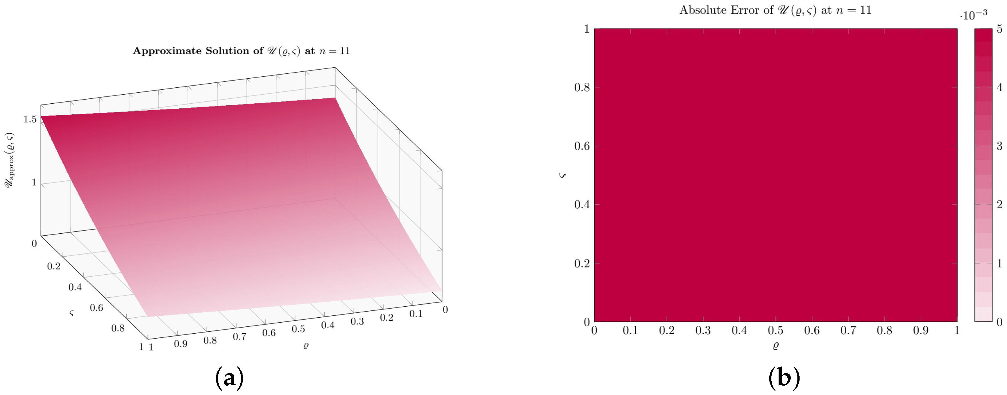
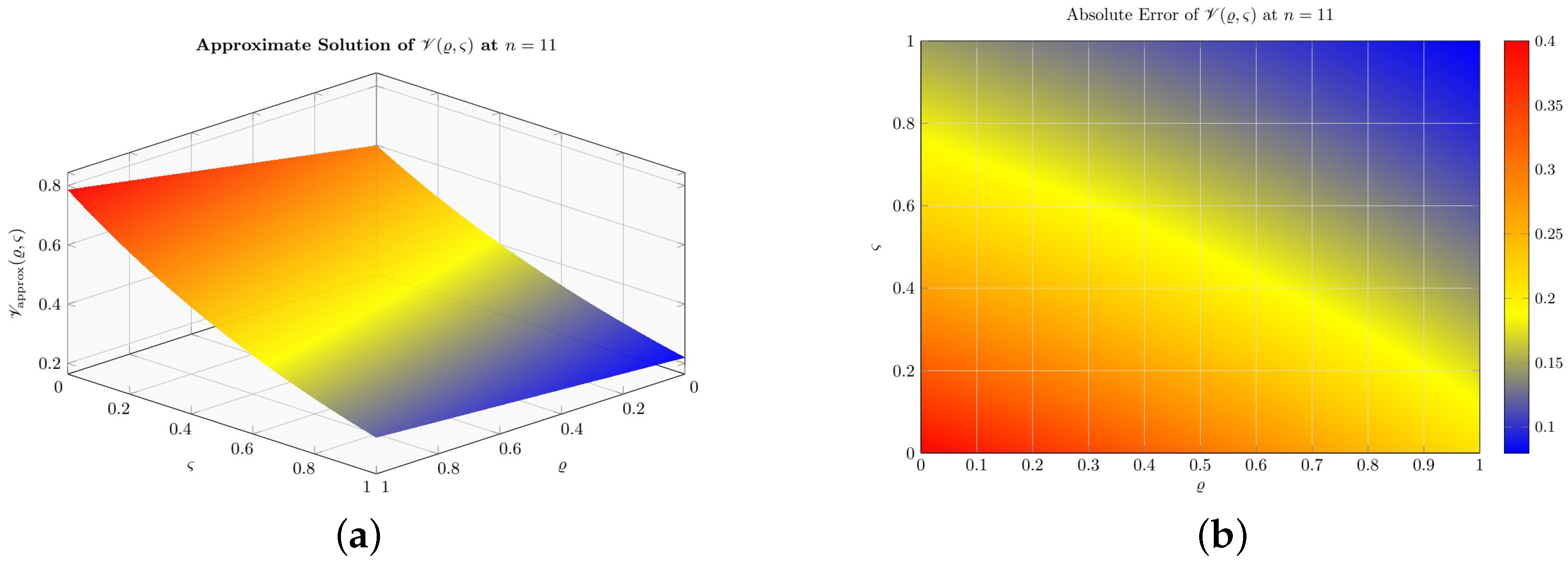
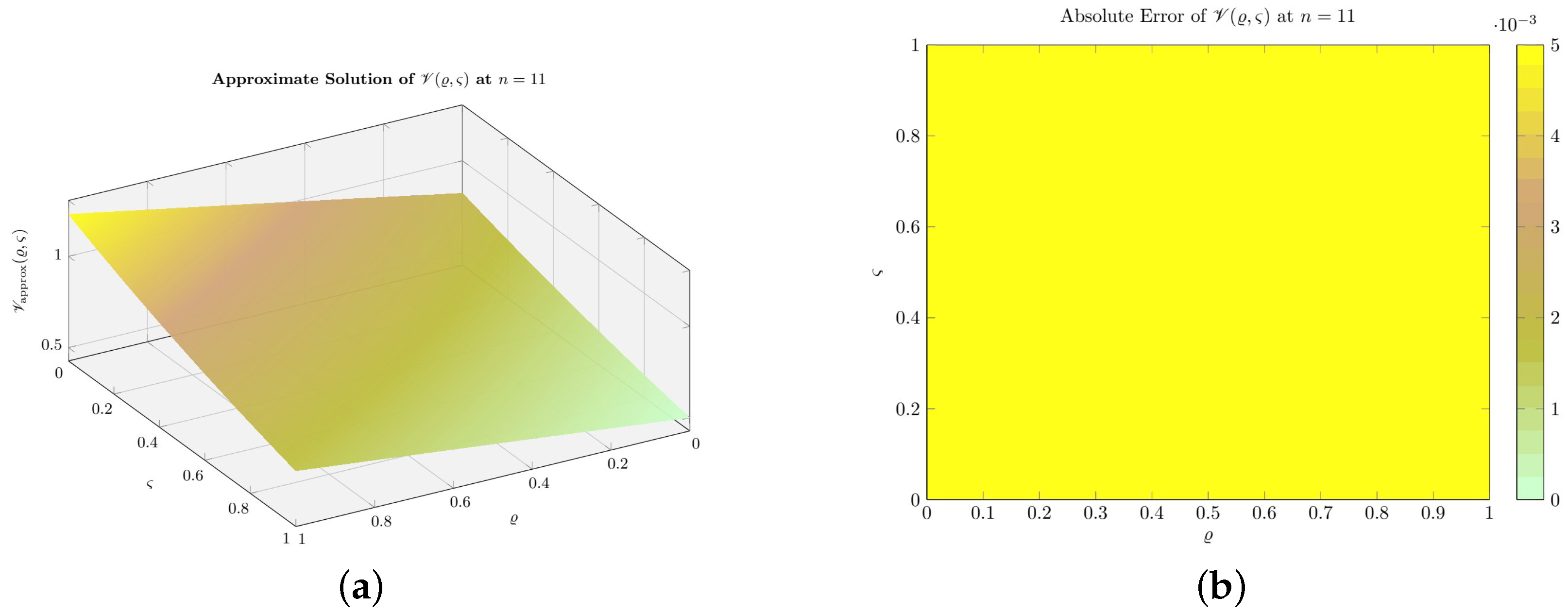
The numerical results provide confirmation of the accuracy and convergence of the proposed method. In Table 1 and Table 2, the errors for solution $\mathcal{U}(\varrho ,\varsigma )$ and $\mathcal{V}(\varrho ,\varsigma )$ in terms of $L_2$ and $L_{\infty }$ are plotted for different values of n and two specific values of ${\alpha }_1(\varrho ,\varsigma )$ and ${\alpha }_2(\varrho ,\varsigma )$, respectively. The tables illustrate a steady decline in the norms of the errors as n is increased, which is indicative of the verification of spectral accuracy. Figure 1 and Figure 2 show results for the approximate and absolute errors when n = 11, with boundary conditions ${\alpha }_1(\varrho ,\varsigma )=0.50+0.2e^{-\varrho \varsigma }$ and ${\alpha }_2(\varrho ,\varsigma )=0.65+0.2sin\left(\varrho \varsigma \right)$.

This numerical experiment validates the spectral correctness of the operational matrix technique. The rapidly decreasing error norms as n increases confirm high-accuracy convergence. The shifted airfoil polynomial-based method effectively approximates solutions for the variable-order time fractional reaction-diffusion coupled system.

Example 2. 

We will consider a variable-order time fractional coupled system of reaction-diffusion equations

$$\begin{array}{cc}\hfill D_{\varsigma }^{{\alpha }_1(\varrho ,\varsigma )}\mathcal{U}(\varrho ,\varsigma )& =a_1{\mathcal{U}}_{\varrho \varrho }+p_1\mathcal{U}+q_1\mathcal{V}+s_1{\mathcal{U}}^2\mathcal{V}+n_1\mathcal{U}\mathcal{V}+m_1\mathcal{U}{\mathcal{V}}^2\hfill \\ \hfill & +{\kappa }_1+{\mathcal{F}}_1(\varrho ,\varsigma ),\varrho \in \mathrm{\Omega },\varsigma >0.\hfill \\ \hfill D_{\varsigma }^{{\alpha }_2(\varrho ,\varsigma )}\mathcal{V}(\varrho ,\varsigma )& =a_2{\mathcal{V}}_{\varrho \varrho }+p_2\mathcal{U}+q_2\mathcal{V}+s_2{\mathcal{U}}^2\mathcal{V}+n_2\mathcal{U}\mathcal{V}+m_2\mathcal{U}{\mathcal{V}}^2\hfill \\ \hfill & +{\kappa }_2+{\mathcal{F}}_2(\varrho ,\varsigma ),\varrho \in \mathrm{\Omega },\varsigma >0,\hfill \end{array}$$

(159)

$\varsigma \in [0,1]$, assuming $a_1=a_2=0.01$, $p_1=0.5$, $q_1=-0.2$, $p_2=-0.4$, $q_2=0.6$, $s_1=s_2=0.05$, $n_1=n_2=0.03$, $m_1=m_2=0.01$, ${\kappa }_1={\kappa }_2=0$. We assume the exact solutions as $\mathcal{U}(\varrho ,\varsigma )=e^{-\varsigma }sin\left(\pi \varrho \right)$ and $\mathcal{V}(\varrho ,\varsigma )=e^{-\varsigma }cos\left(\pi \varrho \right)$, substituting into the model, we compute the source terms

$$\begin{array}{cc}\hfill {\mathcal{F}}_1(\varrho ,\varsigma )& =D_{\varsigma }^{{\alpha }_1(\varrho ,\varsigma )}{e}^{-\varsigma }sin\left(\pi \varrho \right)+0.01e^{-\varsigma }sin\left(\pi \varrho \right)-0.5e^{-\varsigma }sin\left(\pi \varrho \right)-(-0.2)e^{-\varsigma }cos\left(\pi \varrho \right)\hfill \\ \hfill & -0.05{\left[e^{-\varsigma }sin\left(\pi \varrho \right)\right]}^2{e}^{-\varsigma }cos\left(\pi \varrho \right)-0.03e^{-\varsigma }sin\left(\pi \varrho \right)e^{-\varsigma }cos\left(\pi \varrho \right)\hfill \\ \hfill & -0.01e^{-\varsigma }sin\left(\pi \varrho \right){\left[e^{-\varsigma }cos\left(\pi \varrho \right)\right]}^2\hfill \\ \hfill {\mathcal{F}}_2(\varrho ,\varsigma )& =D_{\varsigma }^{{\alpha }_2(\varrho ,\varsigma )}{e}^{-\varsigma }cos\left(\pi \varrho \right)+0.01e^{-\varsigma }cos\left(\pi \varrho \right)-(-0.4)e^{-\varsigma }sin\left(\pi \varrho \right)-0.6e^{-\varsigma }cos\left(\pi \varrho \right)\hfill \\ \hfill & -0.05{\left[e^{-\varsigma }sin\left(\pi \varrho \right)\right]}^2{e}^{-\varsigma }cos\left(\pi \varrho \right)-0.03e^{-\varsigma }sin\left(\pi \varrho \right)e^{-\varsigma }cos\left(\pi \varrho \right)\hfill \\ \hfill & -0.01e^{-\varsigma }sin\left(\pi \varrho \right){\left[e^{-\varsigma }cos\left(\pi \varrho \right)\right]}^2,\hfill \end{array}$$

(160)

with initial conditions

$$\mathcal{U}(\varrho ,0)=sin\left(\pi \varrho \right),\mathcal{U}(\varrho ,0)=cos\left(\pi \varrho \right).$$

(161)

Set 1 having ${\alpha }_1(\varrho ,\varsigma )=0.60+0.15\varrho$ and ${\alpha }_2(\varrho ,\varsigma )=0.70-0.10\varsigma$, while set 2 having ${\alpha }_1(\varrho ,\varsigma )=0.55+0.20sin\left({\displaystyle \frac{\pi \varrho }{2}}\right)$ and ${\alpha }_2(\varrho ,\varsigma )=0.65+0.15cos\left({\displaystyle \frac{\pi \varsigma }{2}}\right)$. Both sets satisfy $0<{\alpha }_j(\varrho ,\varsigma )\le 1for(\varrho ,\varsigma )\in [0,1]\times [0,1]$.

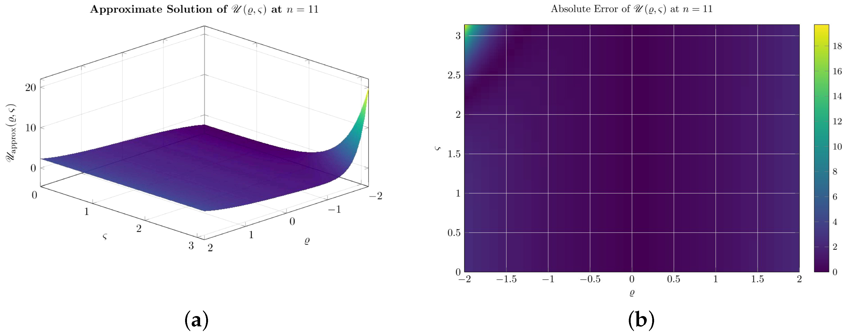
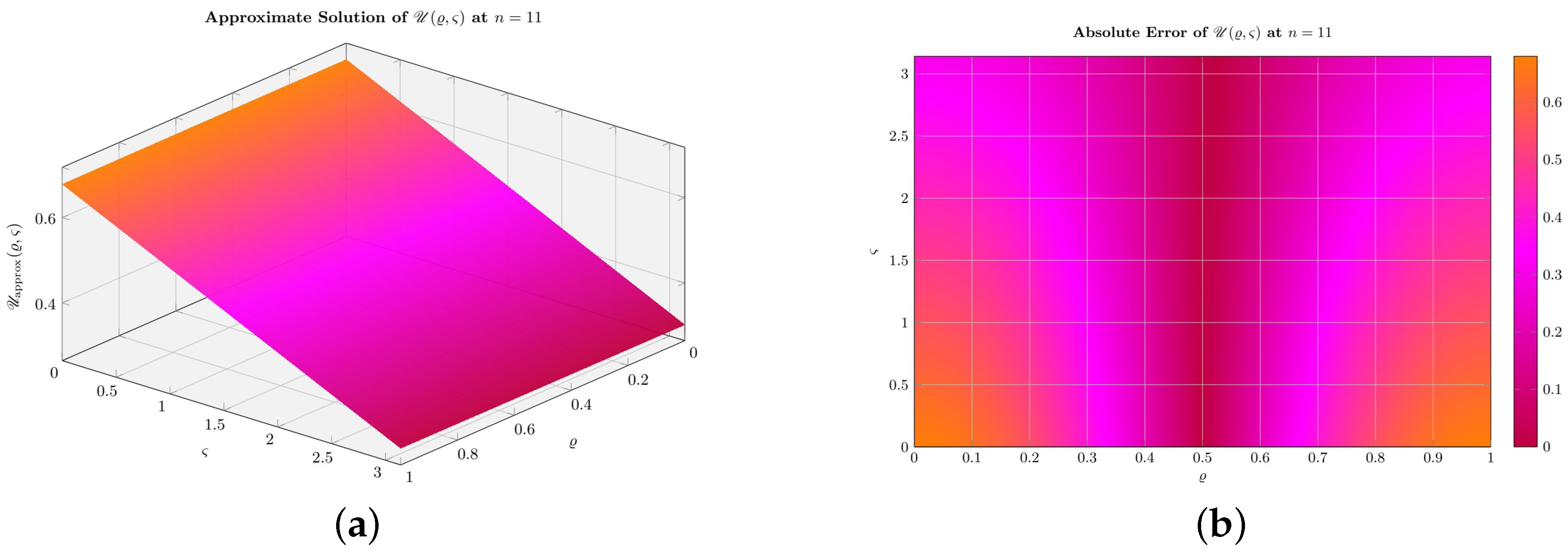
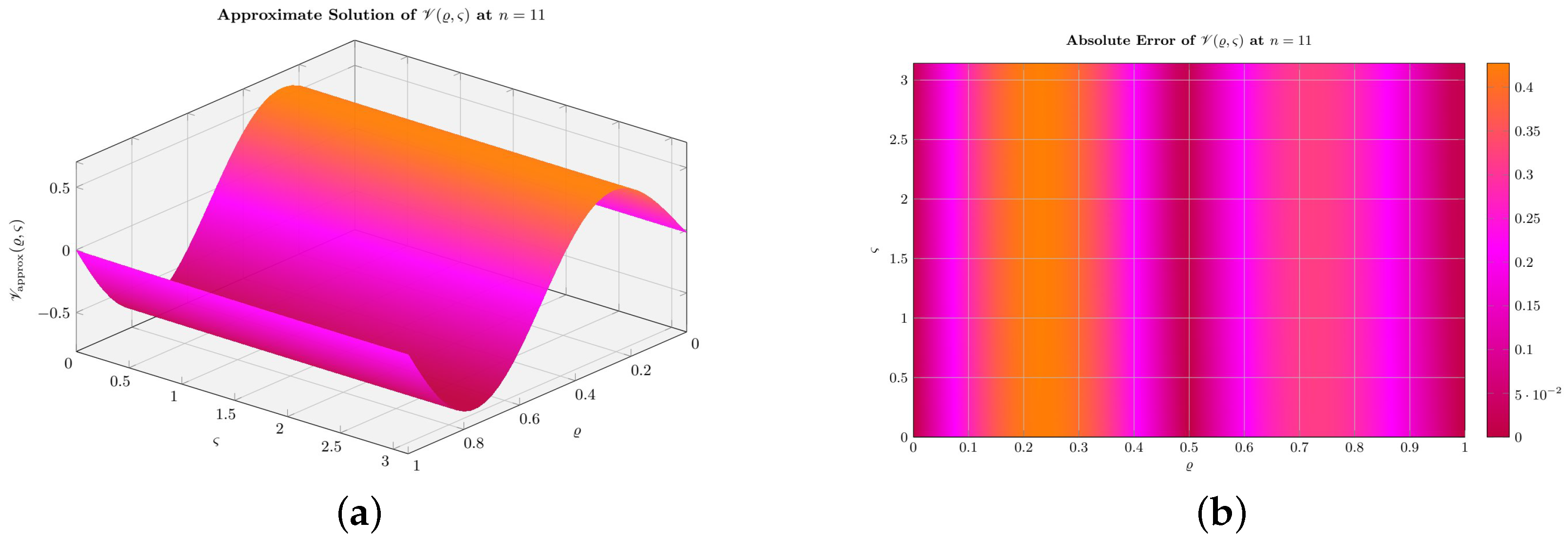
The numerical results provide confirmation of the accuracy and convergence of the presented technique. In

Table 3. Error norms for $\mathcal{U}(\varrho ,\varsigma )$.

n	${{\mathit{L}}_2}^{\mathit{Set}1}$	${{\mathit{L}}_{\mathbf{\infty }}}^{\mathit{Set}1}$	${{\mathit{L}}_{\mathbf{2}}}^{\mathit{Set}2}$	${{\mathit{L}}_{\mathbf{\infty }}}^{\mathit{Set}2}$
3	$2.04\times {10}^{-3}$	$7.61\times {10}^{-4}$	$2.31\times {10}^{-3}$	$8.72\times {10}^{-4}$
5	$1.67\times {10}^{-5}$	$4.58\times {10}^{-6}$	$1.73\times {10}^{-5}$	$4.82\times {10}^{-6}$
7	$6.12\times {10}^{-8}$	$1.12\times {10}^{-8}$	$6.45\times {10}^{-8}$	$1.20\times {10}^{-8}$
9	$1.37\times {10}^{-10}$	$2.85\times {10}^{-11}$	$1.48\times {10}^{-10}$	$3.02\times {10}^{-11}$
11	$3.95\times {10}^{-13}$	$6.11\times {10}^{-14}$	$4.20\times {10}^{-13}$	$6.87\times {10}^{-14}$

and

Table 4. Error norms for $\mathcal{V}(\varrho ,\varsigma )$.

n	${{\mathit{L}}_2}^{\mathit{Set}1}$	${{\mathit{L}}_{\mathbf{\infty }}}^{\mathit{Set}1}$	${{\mathit{L}}_{\mathbf{2}}}^{\mathit{Set}2}$	${{\mathit{L}}_{\mathbf{\infty }}}^{\mathit{Set}2}$
3	$1.82\times {10}^{-3}$	$6.59\times {10}^{-4}$	$1.95\times {10}^{-3}$	$7.04\times {10}^{-4}$
5	$1.23\times {10}^{-5}$	$3.44\times {10}^{-6}$	$1.31\times {10}^{-5}$	$3.61\times {10}^{-6}$
7	$5.01\times {10}^{-8}$	$9.01\times {10}^{-9}$	$5.32\times {10}^{-8}$	$9.73\times {10}^{-9}$
9	$9.92\times {10}^{-11}$	$1.86\times {10}^{-11}$	$1.08\times {10}^{-10}$	$2.01\times {10}^{-11}$
11	$2.85\times {10}^{-13}$	$4.02\times {10}^{-14}$	$3.11\times {10}^{-13}$	$4.67\times {10}^{-14}$

, the errors for the solutions $\mathcal{U}(\varrho ,\varsigma )$ and $\mathcal{V}(\varrho ,\varsigma )$ in terms of $L_2$ and $L_{\infty }$ are presented for different values of n and two specific forms of ${\alpha }_1(\varrho ,\varsigma )$ and ${\alpha }_2(\varrho ,\varsigma )$, respectively. The tables illustrate a consistent decrease in the error norms with increasing n, which verifies the spectral accuracy of the method. Figure 3 and Figure 4 show the approximate and absolute error results for $n=11$, with boundary conditions ${\alpha }_1(\varrho ,\varsigma )=0.60+0.15\varrho$ and ${\alpha }_2(\varrho ,\varsigma )=0.70-0.10\varsigma$.

This numerical experiment validates the spectral correctness of the operational matrix technique. The rapidly decreasing error norms as n increases confirm high-accuracy convergence. The shifted airfoil polynomial-based method effectively approximates solutions for the variable-order time fractional reaction-diffusion coupled system.

Example 3. 

We will consider a variable-order time fractional coupled system of reaction-diffusion equations

$$\begin{array}{cc}\hfill D_{\varsigma }^{{\alpha }_1(\varrho ,\varsigma )}\mathcal{U}(\varrho ,\varsigma )& =a_1{\mathcal{U}}_{\varrho \varrho }+p_1\mathcal{U}+q_1\mathcal{V}+s_1{\mathcal{U}}^2\mathcal{V}+n_1\mathcal{U}\mathcal{V}+m_1\mathcal{U}{\mathcal{V}}^2\hfill \\ \hfill & +{\kappa }_1+{\mathcal{F}}_1(\varrho ,\varsigma ),\varrho \in \mathrm{\Omega },\varsigma >0;\hfill \\ \hfill D_{\varsigma }^{{\alpha }_2(\varrho ,\varsigma )}\mathcal{V}(\varrho ,\varsigma )& =a_2{\mathcal{V}}_{\varrho \varrho }+p_2\mathcal{U}+q_2\mathcal{V}+s_2{\mathcal{U}}^2\mathcal{V}+n_2\mathcal{U}\mathcal{V}+m_2\mathcal{U}{\mathcal{V}}^2\hfill \\ \hfill & +{\kappa }_2+{\mathcal{F}}_2(\varrho ,\varsigma ),\varrho \in \mathrm{\Omega },\varsigma >0,\hfill \end{array}$$

(162)

$\varsigma \in [0,1]$, assuming $a_1=a_2=0.02$, $p_1=0.8$, $q_1=-0.4$, $p_2=-0.5$, $q_2=0.9$, $s_1=s_2=0.08$, $n_1=n_2=0.04$, $m_1=m_2=0.015$, ${\kappa }_1={\kappa }_2=0$. We assume the exact solutions as $\mathcal{U}(\varrho ,\varsigma )=e^{-0.5\varsigma }sin\left(2\pi \varrho \right)$ and $\mathcal{V}(\varrho ,\varsigma )=e^{-0.5\varsigma }cos\left(2\pi \varrho \right)$, substituting into the model, we compute the source terms

$$\begin{array}{cc}\hfill {\mathcal{F}}_1(\varrho ,\varsigma )& =D_{\varsigma }^{{\alpha }_1(\varrho ,\varsigma )}{e}^{-0.5\varsigma }sin\left(2\pi \varrho \right)+4{\pi }^2\left(0.02\right)e^{-0.5\varsigma }sin\left(2\pi \varrho \right)-0.8e^{-0.5\varsigma }sin\left(2\pi \varrho \right)\hfill \\ \hfill & -(-0.4)e^{-0.5\varsigma }cos\left(2\pi \varrho \right)-0.08{\left[e^{-0.5\varsigma }sin\left(2\pi \varrho \right)\right]}^2{e}^{-0.5\varsigma }cos\left(2\pi \varrho \right)\hfill \\ \hfill & -0.04e^{-0.5\varsigma }sin\left(2\pi \varrho \right)e^{-0.5\varsigma }cos\left(2\pi \varrho \right)-0.015e^{-0.5\varsigma }sin\left(2\pi \varrho \right){\left[e^{-0.5\varsigma }cos\left(2\pi \varrho \right)\right]}^2.\hfill \end{array}$$

(163)

$$\begin{array}{cc}\hfill {\mathcal{F}}_2(\varrho ,\varsigma )& =D_{\varsigma }^{{\alpha }_2(\varrho ,\varsigma )}{e}^{-0.5\varsigma }cos\left(2\pi \varrho \right)+4{\pi }^2\left(0.02\right)e^{-0.5\varsigma }cos\left(2\pi \varrho \right)-(-0.5)e^{-0.5\varsigma }sin\left(2\pi \varrho \right)\hfill \\ \hfill & -0.9e^{-0.5\varsigma }cos\left(2\pi \varrho \right)-0.08{\left[e^{-0.5\varsigma }sin\left(2\pi \varrho \right)\right]}^2{e}^{-0.5\varsigma }cos\left(2\pi \varrho \right)\hfill \\ \hfill & -0.04e^{-0.5\varsigma }sin\left(2\pi \varrho \right)e^{-0.5\varsigma }cos\left(2\pi \varrho \right)-0.015e^{-0.5\varsigma }sin\left(2\pi \varrho \right){\left[e^{-0.5\varsigma }cos\left(2\pi \varrho \right)\right]}^2,\hfill \end{array}$$

(164)

with initial conditions

$$\mathcal{U}(\varrho ,0)=sin\left(2\pi \varrho \right),\mathcal{V}(\varrho ,0)=cos\left(2\pi \varrho \right).$$

(165)

Set 1 having ${\alpha }_1(\varrho ,\varsigma )=0.55+0.2\varrho$ and ${\alpha }_2(\varrho ,\varsigma )=0.70-0.15\varsigma$, while set 2 having ${\alpha }_1(\varrho ,\varsigma )=0.60+0.18sin\left(\pi \varrho \right)$ and ${\alpha }_2(\varrho ,\varsigma )=0.65+0.12cos\left(\pi \varsigma \right)$. Both sets satisfy $0<{\alpha }_j(\varrho ,\varsigma )\le 1for(\varrho ,\varsigma )\in [0,1]\times [0,1]$.

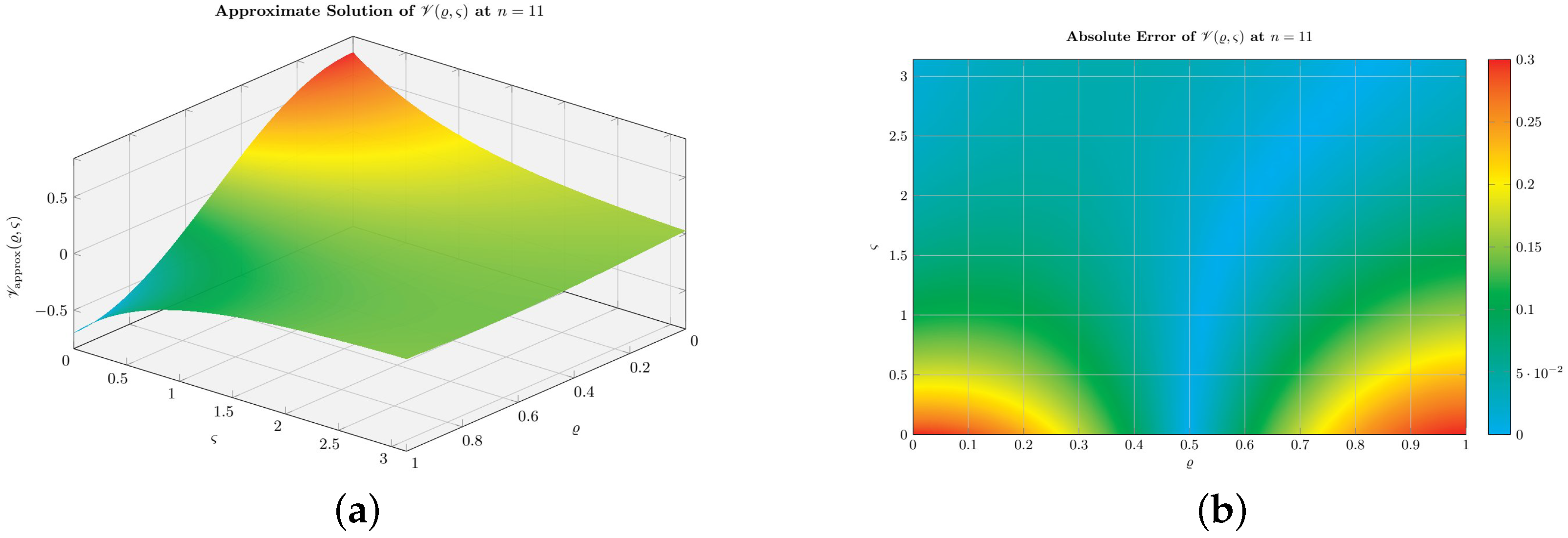
The numerical results provide confirmation of the accuracy and convergence of the presented technique. In

Table 5. Error norms for $\mathcal{U}(\varrho ,\varsigma )$.

n	${{\mathit{L}}_2}^{\mathit{Set}1}$	${{\mathit{L}}_{\mathbf{\infty }}}^{\mathit{Set}1}$	${{\mathit{L}}_{\mathbf{2}}}^{\mathit{Set}2}$	${{\mathit{L}}_{\mathbf{\infty }}}^{\mathit{Set}2}$
3	$2.98\times {10}^{-3}$	$1.12\times {10}^{-3}$	$3.12\times {10}^{-3}$	$1.25\times {10}^{-3}$
5	$1.98\times {10}^{-5}$	$5.34\times {10}^{-6}$	$2.06\times {10}^{-5}$	$5.71\times {10}^{-6}$
7	$8.54\times {10}^{-8}$	$1.73\times {10}^{-8}$	$9.01\times {10}^{-8}$	$1.86\times {10}^{-8}$
9	$2.11\times {10}^{-10}$	$4.12\times {10}^{-11}$	$2.34\times {10}^{-10}$	$4.61\times {10}^{-11}$
11	$5.90\times {10}^{-13}$	$8.24\times {10}^{-14}$	$6.45\times {10}^{-13}$	$9.10\times {10}^{-14}$

and

Table 6. Error norms for $\mathcal{V}(\varrho ,\varsigma )$.

n	${{\mathit{L}}_{\mathbf{2}}}^{\mathit{Set}1}$	${{\mathit{L}}_{\mathbf{\infty }}}^{\mathit{Set}1}$	${{\mathit{L}}_{\mathbf{2}}}^{\mathit{Set}2}$	${{\mathit{L}}_{\mathbf{\infty }}}^{\mathit{Set}2}$
3	$2.65\times {10}^{-3}$	$9.12\times {10}^{-4}$	$2.79\times {10}^{-3}$	$1.03\times {10}^{-3}$
5	$1.42\times {10}^{-5}$	$3.92\times {10}^{-6}$	$1.51\times {10}^{-5}$	$4.21\times {10}^{-6}$
7	$6.09\times {10}^{-8}$	$1.11\times {10}^{-8}$	$6.52\times {10}^{-8}$	$1.19\times {10}^{-8}$
9	$1.26\times {10}^{-10}$	$2.45\times {10}^{-11}$	$1.38\times {10}^{-10}$	$2.68\times {10}^{-11}$
11	$3.72\times {10}^{-13}$	$5.10\times {10}^{-14}$	$4.05\times {10}^{-13}$	$5.78\times {10}^{-14}$

, the errors for the solutions $\mathcal{U}(\varrho ,\varsigma )$ and $\mathcal{V}(\varrho ,\varsigma )$ in terms of $L_2$ and $L_{\infty }$ are presented for different values of n and two specific forms of ${\alpha }_1(\varrho ,\varsigma )$ and ${\alpha }_2(\varrho ,\varsigma )$, respectively. The tables illustrate a steady decrease in the error norms as n increases, confirming the spectral accuracy of the method. Figure 5 and Figure 6 show the results for the approximate and absolute errors when $n=11$, with boundary conditions ${\alpha }_1(\varrho ,\varsigma )=0.55+0.2\varrho$ and ${\alpha }_2(\varrho ,\varsigma )=0.70-0.15\varsigma$.

This numerical experiment validates the spectral correctness of the operational matrix technique. The rapidly decreasing error norms as n increases confirm high-accuracy convergence. The shifted airfoil polynomial-based method effectively approximates solutions for the variable-order time fractional reaction-diffusion coupled system.

Example 4. 

We will consider a variable-order time fractional coupled system of reaction-diffusion equations

$$\begin{array}{cc}\hfill D_{\varsigma }^{{\alpha }_1(\varrho ,\varsigma )}\mathcal{U}(\varrho ,\varsigma )& =a_1{\mathcal{U}}_{\varrho \varrho }+p_1\mathcal{U}+q_1\mathcal{V}+s_1{\mathcal{U}}^2\mathcal{V}+n_1\mathcal{U}\mathcal{V}+m_1\mathcal{U}{\mathcal{V}}^2\hfill \\ \hfill & +{\kappa }_1+{\mathcal{F}}_1(\varrho ,\varsigma ),\varrho \in \mathrm{\Omega },\varsigma >0;\hfill \\ \hfill D_{\varsigma }^{{\alpha }_2(\varrho ,\varsigma )}\mathcal{V}(\varrho ,\varsigma )& =a_2{\mathcal{V}}_{\varrho \varrho }+p_2\mathcal{U}+q_2\mathcal{V}+s_2{\mathcal{U}}^2\mathcal{V}+n_2\mathcal{U}\mathcal{V}+m_2\mathcal{U}{\mathcal{V}}^2\hfill \\ \hfill & +{\kappa }_2+{\mathcal{F}}_2(\varrho ,\varsigma ),\varrho \in \mathrm{\Omega },\varsigma >0,\hfill \end{array}$$

(166)

$\varsigma \in [0,1]$, assuming $a_1=a_2=0.015$, $p_1=0.9$, $q_1=-0.45$, $p_2=-0.45$, $q_2=0.85$, $s_1=s_2=0.07$, $n_1=n_2=0.035$, $m_1=m_2=0.012$, ${\kappa }_1={\kappa }_2=0$. We assume the exact solutions as $\mathcal{U}(\varrho ,\varsigma )=sin\left(\pi \varrho \right)sin\left(\varsigma \right)$ and $\mathcal{V}(\varrho ,\varsigma )=sin\left(2\pi \varrho \right)cos\left(\varsigma \right)$, substituting into the model, we compute the source terms

$$\begin{array}{cc}\hfill {\mathcal{F}}_1(\varrho ,\varsigma )& =D_{\varsigma }^{{\alpha }_1(\varrho ,\varsigma )}sin\left(\pi \varrho \right)sin\left(\varsigma \right)+0.015{\pi }^{2}sin\left(\pi \varrho \right)sin\left(\varsigma \right)-0.9sin\left(\pi \varrho \right)sin\left(\varsigma \right)\hfill \\ \hfill & -(-0.45)sin\left(2\pi \varrho \right)cos\left(\varsigma \right)-0.07{\left[sin\left(\pi \varrho \right)sin\left(\varsigma \right)\right]}^{2}sin\left(2\pi \varrho \right)cos\left(\varsigma \right)\hfill \\ \hfill & -0.035sin\left(\pi \varrho \right)sin\left(\varsigma \right)sin\left(2\pi \varrho \right)cos\left(\varsigma \right)-sin\left(\pi \varrho \right)sin\left(\varsigma \right){\left[sin\left(2\pi \varrho \right)cos\left(\varsigma \right)\right]}^2;\hfill \\ \hfill {\mathcal{F}}_2(\varrho ,\varsigma )& =D_{\varsigma }^{{\alpha }_2(\varrho ,\varsigma )}sin\left(2\pi \varrho \right)cos\left(\varsigma \right)+4\left(0.015\right){\pi }^{2}sin\left(2\pi \varrho \right)cos\left(\varsigma \right)-(-0.45)sin\left(\pi \varrho \right)sin\left(\varsigma \right)\hfill \\ \hfill & -0.85sin\left(2\pi \varrho \right)cos\left(\varsigma \right)-0.07{\left[sin\left(\pi \varrho \right)sin\left(\varsigma \right)\right]}^{2}sin\left(2\pi \varrho \right)cos\left(\varsigma \right)\hfill \\ \hfill & -0.035sin\left(\pi \varrho \right)sin\left(\varsigma \right)sin\left(2\pi \varrho \right)cos\left(\varsigma \right)-0.012sin\left(\pi \varrho \right)sin\left(\varsigma \right){\left[sin\left(2\pi \varrho \right)cos\left(\varsigma \right)\right]}^2,\hfill \end{array}$$

(167)

with initial conditions

$$\mathcal{U}(\varrho ,0)=0,\mathcal{V}(\varrho ,0)=sin\left(2\pi \varrho \right).$$

(168)

Set 1 having ${\alpha }_1(\varrho ,\varsigma )=0.52+0.22\varrho$ and ${\alpha }_2(\varrho ,\varsigma )=0.68-0.12\varsigma$, while Set 2 having ${\alpha }_1(\varrho ,\varsigma )=0.58+0.18sin\left(\pi \varrho \right)$ and ${\alpha }_2(\varrho ,\varsigma )=0.62+0.14cos\left(\pi \varsigma 2\right)$. Both sets satisfy $0<{\alpha }_j(\varrho ,\varsigma )\le 1for(\varrho ,\varsigma )\in [0,1]\times [0,1]$.

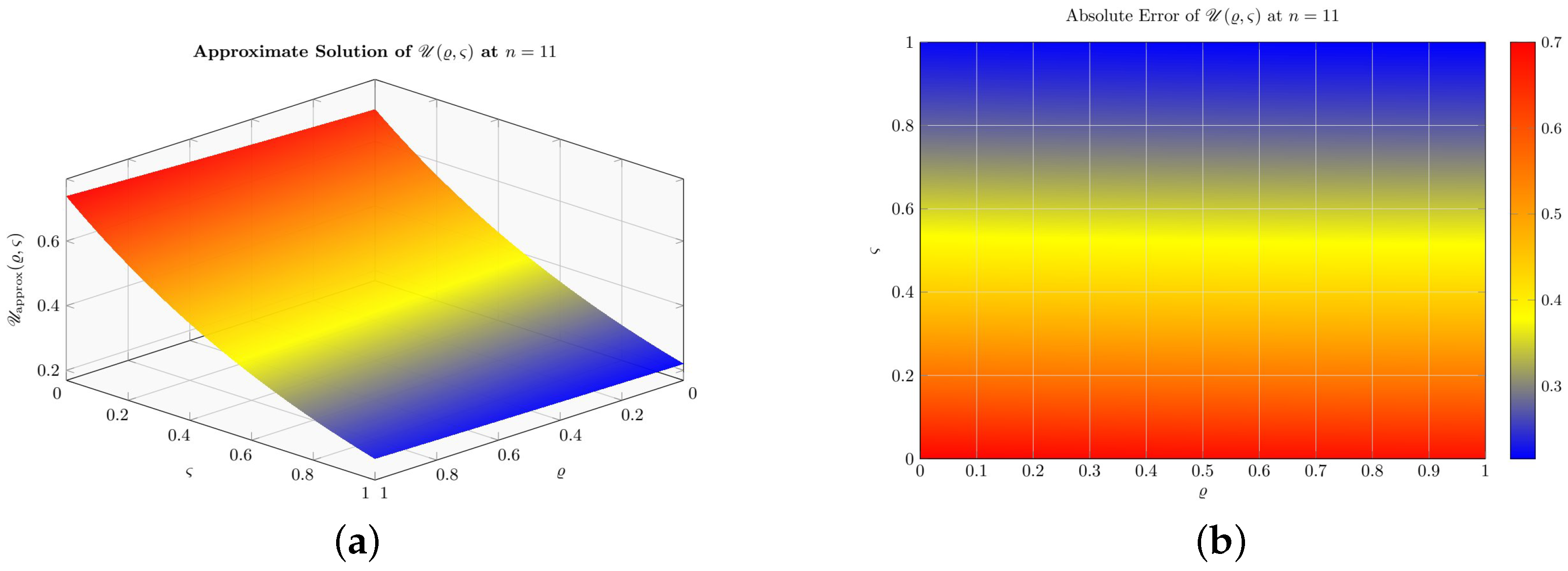
The numerical results provide confirmation of the accuracy and convergence of the presented technique. In

Table 7. Error norms for $\mathcal{U}(\varrho ,\varsigma )$.

n	${{\mathit{L}}_2}^{\mathit{Set}1}$	${{\mathit{L}}_{\mathbf{\infty }}}^{\mathit{Set}1}$	${{\mathit{L}}_{\mathbf{2}}}^{\mathit{Set}\mathbf{2}}$	${{\mathit{L}}_{\mathbf{\infty }}}^{\mathbf{Set}\mathbf{2}}$
3	$2.50\times {10}^{-3}$	$8.50\times {10}^{-4}$	$2.70\times {10}^{-3}$	$9.20\times {10}^{-4}$
5	$1.50\times {10}^{-5}$	$4.20\times {10}^{-6}$	$1.60\times {10}^{-5}$	$4.50\times {10}^{-6}$
7	$7.00\times {10}^{-8}$	$1.40\times {10}^{-8}$	$7.60\times {10}^{-8}$	$1.60\times {10}^{-8}$
9	$1.90\times {10}^{-10}$	$3.50\times {10}^{-11}$	$2.00\times {10}^{-10}$	$3.80\times {10}^{-11}$
11	$5.20\times {10}^{-13}$	$7.90\times {10}^{-14}$	$5.80\times {10}^{-13}$	$8.60\times {10}^{-14}$

and

Table 8. Error norms for $\mathcal{V}(\varrho ,\varsigma )$.

n	${{\mathit{L}}_2}^{\mathit{Set}1}$	${{\mathit{L}}_{\mathbf{\infty }}}^{\mathit{Set}1}$	${{\mathit{L}}_{\mathbf{2}}}^{\mathit{Set}2}$	${{\mathit{L}}_{\mathbf{\infty }}}^{\mathit{Set}\mathbf{2}}$
3	$2.10\times {10}^{-3}$	$7.20\times {10}^{-4}$	$2.30\times {10}^{-3}$	$7.80\times {10}^{-4}$
5	$1.10\times {10}^{-5}$	$3.00\times {10}^{-6}$	$1.20\times {10}^{-5}$	$3.20\times {10}^{-6}$
7	$5.50\times {10}^{-8}$	$1.00\times {10}^{-8}$	$5.90\times {10}^{-8}$	$1.10\times {10}^{-8}$
9	$1.20\times {10}^{-10}$	$2.20\times {10}^{-11}$	$1.30\times {10}^{-10}$	$2.50\times {10}^{-11}$
11	$3.30\times {10}^{-13}$	$4.50\times {10}^{-14}$	$3.70\times {10}^{-13}$	$5.00\times {10}^{-14}$

, the errors for the solutions $\mathcal{U}(\varrho ,\varsigma )$ and $\mathcal{V}(\varrho ,\varsigma )$ in terms of $L_2$ and $L_{\infty }$ are presented for different values of n and two specific forms of ${\alpha }_1(\varrho ,\varsigma )$ and ${\alpha }_2(\varrho ,\varsigma )$, respectively. The tables illustrate a steady decrease in the norms of the errors as n increases, verifying the spectral accuracy of the method. Figure 7 and Figure 8 present the results for the approximate and absolute errors when $n=11$, with boundary conditions ${\alpha }_1(\varrho ,\varsigma )=0.52+0.22\varrho$ and ${\alpha }_2(\varrho ,\varsigma )=0.68-0.12\varsigma$.

This numerical experiment validates the spectral correctness of the operational matrix technique. The rapidly decreasing error norms as n increases confirm high-accuracy convergence. The shifted airfoil polynomial-based method effectively approximates solutions for the variable-order time fractional reaction-diffusion coupled system.

7. Conclusions

In the present study, we have explored a numerical methodology for approximating solutions to variable-order time-fractional reaction–diffusion coupled equations, with the fractional derivatives defined in the Caputo sense. The analysis establishes both the existence and uniqueness of solutions, while also examining Ulam–Hyers stability to confirm the robustness of the model. For the construction of the numerical scheme, shifted second-kind Airfoil polynomials were utilized as basis functions within a spectral framework. Corresponding operational matrices for both integer-order and variable-order fractional operators were systematically derived, enabling the transformation of the original system into an equivalent algebraic system via the collocation approach.

The proposed scheme has been validated by illustrative examples for its accuracy and efficiency, thus confirming that the method can deliver results that are highly reliable as compared to other current techniques. The proposed method not only simplifies the computational process but also guarantees stability and precision in the results of coupled nonlinear fractional systems. For future work, the research can be broadened to explore multi-dimensional (VO) fractional reaction-diffusion systems and other intricate coupled models with variable coefficients, by means of advanced numerical techniques for wider usage.

References

1. Hilfer, R. Applications of Fractional Calculus in Physics; World Scientific: Singapore, 2000. [Google Scholar]
2. Cheow, Y.H.; Ng, K.H.; Phang, C.; Ng, K.H. The application of fractional calculus in economic growth modelling: An approach based on regression analysis. Heliyon 2024, 10, e35379. [Google Scholar] [CrossRef] [PubMed]
3. Zhou, Y. Basic Theory of Fractional Differential Equations; World Scientific: Singapore, 2023. [Google Scholar]
4. Hattaf, K. On the stability and numerical scheme of fractional differential equations with application to biology. Computation 2022, 10, 97. [Google Scholar] [CrossRef]
5. Younis, M.; Ahmad, H.; Ozturk, M.; Din, F.U.; Qasim, M. Unveiling fractional-order dynamics: A new method for analyzing Rössler Chaos. J. Comput. Appl. Math. 2025, 468, 116639. [Google Scholar] [CrossRef]
6. Hammouch, Z.; Yavuz, M.; Özdemir, N. Numerical solutions and synchronization of a variable-order fractional chaotic system. Math. Model. Numer. Simul. Appl. 2021, 1, 11–23. [Google Scholar] [CrossRef]
7. Sun, H.; Chang, A.; Zhang, Y.; Chen, W. A review on variable-order fractional differential equations: Mathematical foundations, physical models, numerical methods and applications. Fract. Calc. Appl. Anal. 2019, 22, 27–59. [Google Scholar] [CrossRef]
8. Younis, M.; Ahmad, H.; Ozturk, M.; Singh, D. A novel approach to the convergence analysis of chaotic dynamics in fractional order Chua’s attractor model employing fixed points. Alex. Eng. J. 2025, 110, 363–375. [Google Scholar] [CrossRef]
9. Ahmad, H.; Peerzada, M.A.; Wardah, W. A Fixed Point Approach to the Existence and Uniqueness of Solutions for Thomas Cyclically Symmetric Attractor. Sak. J. Math. 2025, 1, 22–36. [Google Scholar]
10. Yu, J.; Feng, Y. On the generalized time fractional reaction–diffusion equation: Lie symmetries, exact solutions and conservation laws. Chaos Solitons Fractals 2024, 182, 114855. [Google Scholar] [CrossRef]
11. Ghafoor, A.; Fiaz, M.; Hussain, M.; Ullah, A.; Ismail, E.A.A.; Awwad, F.A. Dynamics of the time-fractional reaction–diffusion coupled equations in biological and chemical processes. Sci. Rep. 2024, 14, 7549. [Google Scholar] [CrossRef]
12. Berkenstock, D.; Alonso, J.; Lessard, L. Orthonormal Polynomial Bases for Airfoil Design. In Proceedings of the 2024 IEEE Aerospace Conference, Big Sky, MT, USA, 2–9 March 2024; pp. 1–9. [Google Scholar]
13. Benchouk, M.; Khelifa, S. A modified Adomian decomposition method with orthogonal Airfoil polynomials for solving non-homogeneous differential equations. Res. Math. 2025, 12, 2526879. [Google Scholar] [CrossRef]
14. Wang, X.; Luo, D.; Zhu, Q. Ulam-Hyers stability of caputo type fuzzy fractional differential equations with time-delays. Chaos Solitons Fractals 2022, 156, 111822. [Google Scholar] [CrossRef]
15. Al-khateeb, A.; Zureigat, H.; Ala’yed, O.; Bawaneh, S. Ulam–Hyers stability and uniqueness for nonlinear sequential fractional differential equations involving integral boundary conditions. Fractal Fract. 2021, 5, 235. [Google Scholar] [CrossRef]
16. Kumar, S.; Chauhan, R.P.; Momani, S.; Hadid, S. A study of a modified nonlinear dynamical system with fractal-fractional derivative. Int. J. Numer. Methods Heat Fluid Flow 2022, 52, 2620–2639. [Google Scholar] [CrossRef]
17. Alzaid, S.S.; Kumar, R.; Chauhan, R.P.; Kumar, S. Laguerre wavelet method for fractional predator–prey population model. Fractals 2022, 30, 2240215. [Google Scholar] [CrossRef]
18. Kumar, S.; Chauhan, R.P.; Abdel-Aty, A.H.; Abdelwahab, S.F. A study on fractional tumour–immune–vitamins model for intervention of vitamins. Results Phys. 2022, 33, 104963. [Google Scholar] [CrossRef]
19. Hassani, H.; Machado, J.A.T.; Naraghirad, E. An efficient numerical technique for variable order time fractional nonlinear Klein-Gordon equation. Appl. Numer. Math. 2020, 154, 260–272. [Google Scholar] [CrossRef]
20. Hassani, H.; Machado, J.A.T.; Avazzadeh, Z.; Naraghirad, E. Generalized shifted Chebyshev polynomials: Solving a general class of nonlinear variable order fractional PDE. Commun. Nonlinear Sci. Numer. Simul. 2020, 85, 105229. [Google Scholar] [CrossRef]
21. Hassani, H.; Avazzadeh, Z.; Machado, J.A.T. Numerical approach for solving variable-order space–time fractional telegraph equation using transcendental Bernstein series. Eng. Comput. 2020, 36, 867–878. [Google Scholar] [CrossRef]
22. Chen, Y.; Zhang, J.; Pan, C. Numerical approximation of a variable-order time fractional advection-reaction-diffusion model via shifted Gegenbauer polynomials. AIMS Math. 2022, 7, 15612–15632. [Google Scholar] [CrossRef]
23. Hosseininia, M.; Heydari, M.H.; Rouzegar, J.; Cattani, C. A meshless method to solve nonlinear variable-order time fractional 2D reaction–diffusion equation involving Mittag-Leffler kernel. Eng. Comput. 2021, 37, 731–743. [Google Scholar] [CrossRef]
24. Kashif, M.; Pandey, P.; Jafari, H. A novel numerical manner for non-linear coupled variable order reaction-diffusion equation. Therm. Sci. 2023, 27, 353–363. [Google Scholar] [CrossRef]
25. Coronel-Escamilla, A.; Gómez-Aguilar, J.F.; Torres, L.; Escobar-Jiménez, R.F. A numerical solution for a variable-order reaction–diffusion model by using fractional derivatives with non-local and non-singular kernel. Phys. A Stat. Mech. Appl. 2018, 491, 406–424. [Google Scholar] [CrossRef]
26. Khalighi, M.; Amirianmatlob, M.; Malek, A. A new approach to solving multiorder time-fractional advection–diffusion–reaction equations using BEM and Chebyshev matrix. Math. Methods Appl. Sci. 2021, 44, 2964–2984. [Google Scholar] [CrossRef]
27. Kumar, S.; Gupta, V.; Zeidan, D. An efficient collocation technique based on operational matrix of fractional-order Lagrange polynomials for solving the space-time fractional-order partial differential equations. Appl. Numer. Math. 2024, 204, 249–264. [Google Scholar] [CrossRef]
28. Doha, E.H.; Bhrawy, A.H.; Ezz-Eldien, S.S. A Chebyshev spectral method based on operational matrix for initial and boundary value problems of fractional order. Comput. Math. Appl. 2011, 62, 2364–2373. [Google Scholar] [CrossRef]
29. Maleknejad, K.; Basirat, B.; Hashemizadeh, E. A Bernstein operational matrix approach for solving a system of high order linear Volterra–Fredholm integro-differential equations. Math. Comput. Model. 2012, 55, 1363–1372. [Google Scholar] [CrossRef]
30. Li, Z.; Huang, X.; Liu, Y. Initial-boundary value problems for coupled systems of time-fractional diffusion equations. Fract. Calc. Appl. Anal. 2023, 26, 533–566. [Google Scholar] [CrossRef]
31. Kashif, M.; Singh, M. Existence, uniqueness and Ulam–Hyers stability result for variable order fractional predator-prey system and it’s numerical solution. Appl. Numer. Math. 2025, 207, 193–209. [Google Scholar] [CrossRef]
32. Chefnaj, N.; Hilal, K.; Kajouni, A. The existence, uniqueness and Ulam–Hyers stability results of a hybrid coupled system with Ψ-Caputo fractional derivatives. J. Appl. Math. Comput. 2024, 70, 2209–2224. [Google Scholar] [CrossRef]
33. Irshad, N.; Shah, R.; Liaquat, K.; Mahmoud, E.E. Stability analysis of solutions to the time–fractional nonlinear Schrödinger equations. Int. J. Theor. Phys. 2025, 64, 128. [Google Scholar] [CrossRef]
34. Shah, R.; Bibi, H.; Irshad, N.; Abbasi, H.I. On Hyers–Ulam stability of a class of impulsive Hammerstein integral equations. Filomat 2025, 39, 2405–2416. [Google Scholar] [CrossRef]
35. Irshad, N.; Shah, R.; Liaquat, K. Hyers–Ulam–Rassias stability for a class of nonlinear convolution integral equations. Filomat 2025, 39, 4207–4220. [Google Scholar] [CrossRef]
36. Abdelkawy, M.A.; Taha, T.M. An operational matrix of fractional derivatives of Laguerre polynomials. Walailak J. Sci. Technol. (WJST) 2014, 11, 1041–1055. [Google Scholar]
37. Srivastava, H.M.; Shah, F.A.; Abass, R. An application of the Gegenbauer wavelet method for the numerical solution of the fractional Bagley-Torvik equation. Russ. J. Math. Phys. 2019, 26, 77–93. [Google Scholar] [CrossRef]
38. Zhang, P. A second order box-type scheme for fractional sub-diffusion equation with spatially variable coefficient under Neumann boundary conditions. Adv. Differ. Equ. 2017, 2017, 144. [Google Scholar] [CrossRef][Green Version]
39. Carmona, J.; Colorado, E.; Leonori, T.; Ortega, A. Regularity of solutions to a fractional elliptic problem with mixed Dirichlet–Neumann boundary data. Adv. Calc. Var. 2021, 14, 521–539. [Google Scholar] [CrossRef]
40. Singh, A.; Kumar, S. Error analysis of a high-order fully discrete method for two-dimensional time-fractional convection-diffusion equations exhibiting weak initial singularity. Numer. Algorithms 2025, 99, 251–284. [Google Scholar] [CrossRef]
41. Almeida, R.; Tavares, D.; Torres, D.F.M. The Variable-Order Fractional Calculus of Variations; Springer: Berlin/Heidelberg, Germany, 2019. [Google Scholar]
42. Chen, Y.; Liu, L.; Li, B.; Sun, Y. Numerical solution for the variable order linear cable equation with Bernstein polynomials. Appl. Math. Comput. 2014, 238, 329–341. [Google Scholar] [CrossRef]
43. Heydari, M.H.; Avazzadeh, Z.; Cattani, C. Numerical solution of variable-order space-time fractional KdV–Burgers–Kuramoto equation by using discrete Legendre polynomials. Eng. Comput. 2022, 38, 859–869. [Google Scholar] [CrossRef]
44. Srivastava, H.M.; Izadi, M. Generalized shifted airfoil polynomials of the second kind to solve a class of singular electrohydrodynamic fluid model of fractional order. Fractal Fract. 2023, 7, 94. [Google Scholar] [CrossRef]
45. Derakhshan, M.H. Existence, uniqueness, Ulam–Hyers stability and numerical simulation of solutions for variable order fractional differential equations in fluid mechanics. J. Appl. Math. Comput. 2022, 68, 403–429. [Google Scholar] [CrossRef]
Figure 1. For n = 11 , the approximate solution (a) and the absolute error (b) of U ( ϱ , ς ) are computed with α 1 ( ϱ , ς ) = 0.50 + 0.2 e ϱ ς and α 2 ( ϱ , ς ) = 0.65 + 0.2 sin ( ϱ ς ) for Example 1.
Fractalfract 10 00151 g001
Figure 2. For n = 11 , the approximate solution (a) and the absolute error (b) of V ( ϱ , ς ) are computed with α 1 ( ϱ , ς ) = 0.50 + 0.2 e ϱ ς and α 2 ( ϱ , ς ) = 0.65 + 0.2 sin ( ϱ ς ) for Example 1.
Fractalfract 10 00151 g002
Figure 3. For n = 11 , the approximate solution (a) and the absolute error (b) of U ( ϱ , ς ) are computed with α 1 ( ϱ , ς ) = 0.60 + 0.15 ϱ and α 2 ( ϱ , ς ) = 0.70 0.10 ς for Example 2.
Fractalfract 10 00151 g003
Figure 4. For n = 11 , the approximate solution (a) and the absolute error (b) of V ( ϱ , ς ) are computed with α 1 ( ϱ , ς ) = 0.60 + 0.15 ϱ and α 2 ( ϱ , ς ) = 0.70 0.10 ς for Example 2.
Fractalfract 10 00151 g004
Figure 5. For n = 11 , the approximate solution (a) and the absolute error (b) of U ( ϱ , ς ) are computed with α 1 ( ϱ , ς ) = 0.55 + 0.2 ϱ and α 2 ( ϱ , ς ) = 0.70 0.15 ς for Example 3.
Fractalfract 10 00151 g005
Figure 6. For n = 11 , the approximate solution (a) and the absolute error (b) of V ( ϱ , ς ) are computed with α 1 ( ϱ , ς ) = 0.55 + 0.2 ϱ and α 2 ( ϱ , ς ) = 0.70 0.15 ς for Example 3.
Fractalfract 10 00151 g006
Figure 7. For n = 11 , the approximate solution (a) and the absolute error (b) of U ( ϱ , ς ) are computed with α 1 ( ϱ , ς ) = 0.52 + 0.22 ϱ and α 2 ( ϱ , ς ) = 0.68 0.12 ς for Example 4.
Fractalfract 10 00151 g007
Figure 8. For n = 11 , the approximate solution (a) and the absolute error (b) of V ( ϱ , ς ) are computed with α 1 ( ϱ , ς ) = 0.52 + 0.22 ϱ and α 2 ( ϱ , ς ) = 0.68 0.12 ς for Example 4.
Fractalfract 10 00151 g008