Interpretable Ensemble Machine Learning for Liquefaction Risk Prediction

Abstract

This paper presents a comprehensive machine learning (ML) framework for predicting liquefaction risk, a crucial aspect of seismic hazard assessment. A benchmark geotechnical dataset with multi-dimensional input features was used to evaluate several ML classifiers, followed by hyperparameter optimization through stratified 5-fold cross-validation. Optimized models were combined into a soft Voting Ensemble to enhance stability and accuracy of liquefaction potential prediction. The proposed ensemble model achieved a mean accuracy of 90.12% and a recall of 97.23%, outperforming individual models in most folds. The ensemble’s effectiveness was further evidenced by its precision-recall (PR) and receiver operating characteristic (ROC) curves, with areas under the curve (AUC) of 0.962 and 0.931, respectively—closely matching those of the Gradient Boosting classifier, indicating comparable discriminatory performance. Additionally, SHapley Additive exPlanations (SHAP) analysis was conducted on the ensemble model to assess contributions of each geotechnical inputs to the predictions, revealing that normalized shear wave velocity ($V_{S1}$) as the most influential variable in liquefaction prediction. The proposed framework demonstrates a robust, interpretable, and performance-consistent approach for liquefaction risk assessment.

1. Introduction

Soil liquefaction is a critical geotechnical phenomenon that typically occurs during seismic events, when granular soils temporarily lose strength and stiffness due to increased pore-water pressure and reduced effective stress [1]. It most commonly affects loose to moderately dense granular soils with poor drainage, such as silty sands or sands with impermeable layers, posing substantial risks to infrastructure stability and public safety. Accurately predicting liquefaction-prone sites is therefore crucial for mitigating seismic hazards.

In geotechnical engineering, the complexity of soil behavior often necessitates empirical or semi-empirical approaches to estimate soil performance under dynamic loading [2]. Traditional liquefaction assessment methods, such as stress-based, strain-based, and energy-based approaches [1,3,4,5], rely heavily on in-situ tests like the Standard Penetration Test (SPT) and Cone Penetration Test (CPT) [4,6,7,8,9]. However, these methods have inherent limitations, including simplifying assumptions, site-specific calibration, and the logistical and financial costs associated with field testing. Even $V_S$-based liquefaction analyses [10,11], while valuable, are limited to site specific conditions such as shallow groundwater tables and limited depth ranges.

To overcome these limitations, machine learning (ML) algorithms have emerged as powerful tools capable of capturing complex, non-linear relationships in geotechnical data. Goh [12] pioneered its use in liquefaction prediction using neural networks trained on SPT data. Since then, numerous studies have demonstrated ML’s potential for soil classification, property prediction, and ground behavior forecasting [2,13,14,15,16,17]. However, most studies focused on single ML algorithms or homogeneous ensembles (e.g., Random Forest, Gradient Boosting), limiting model diversity and generalization [18].

This study introduces a heterogeneous ensemble learning framework that integrates multiple types of ML algorithms to enhance prediction robustness and accuracy. By combining diverse base learners, the ensemble model capitalizes on the strengths of different algorithms while compensating for their individual weaknesses.

Liquefaction datasets typically include input variables derived from SPT, CPT, or shear wave velocity ($V_S)$ measurements [2,18,19]. Jas and Dodagoudar [18] highlighted the importance of incorporating a broad range of geotechnical and seismic variables to improve predictive performance. However, small dataset with numerous features often increase the risk of overfitting, where models perform well on training data but fail to generalize to unseen samples. To avoid this issue, the present study employs a stratified five-fold cross-validation (CV) procedure, ensuring reliable model evaluation across different subsets of data. As demonstrated by Demir and Sahin [20], CV provides a more objective assessment of model performance compared to single train-test splits.

Hyperparameter optimization further enhances model reliability by identifying parameter combinations that maximize performance on a validation dataset. The importance of hyperparameter optimization in liquefaction analysis has been highlighted by Ozsagir, Erden [21] and Kurnaz, Erden [22].

A persistent challenge in using advanced non-linear ML algorithms lies in their interpretability, particularly when ensemble models are employed. To ensure transparency, this study utilizes SHapley Additive exPlanations (SHAP), which quantify the contribution of each geotechnical input to the final prediction [23].

Despite growing research on ML-based liquefaction assessment, few studies have explored the synergy of heterogeneous ensembles with robust validation and interpretability frameworks. To address this gap, this paper aims to: (1) assembling a benchmark dataset incorporating diverse geotechnical and seismic features; (2) investigating the effectiveness of various base ML algorithms; (3) systematically optimizing hyperparameters of base models; (4) constructing a soft voting ensemble to leverage model strengths; and (5) analyzing feature importance using SHAP. A stratified 5-fold CV was applied throughout all stages of the study to ensure the reliability of the ML results and avoid overfitting or randomness.

This study develops a heterogeneous, recall-optimized ensemble with nested cross-validation and SHAP interpretability to deliver high-recall liquefaction classification while preserving discrimination (ROC/PR AUC), thereby aligning data-driven inference with established geotechnical mechanisms.

2. Materials

2.1. Dataset

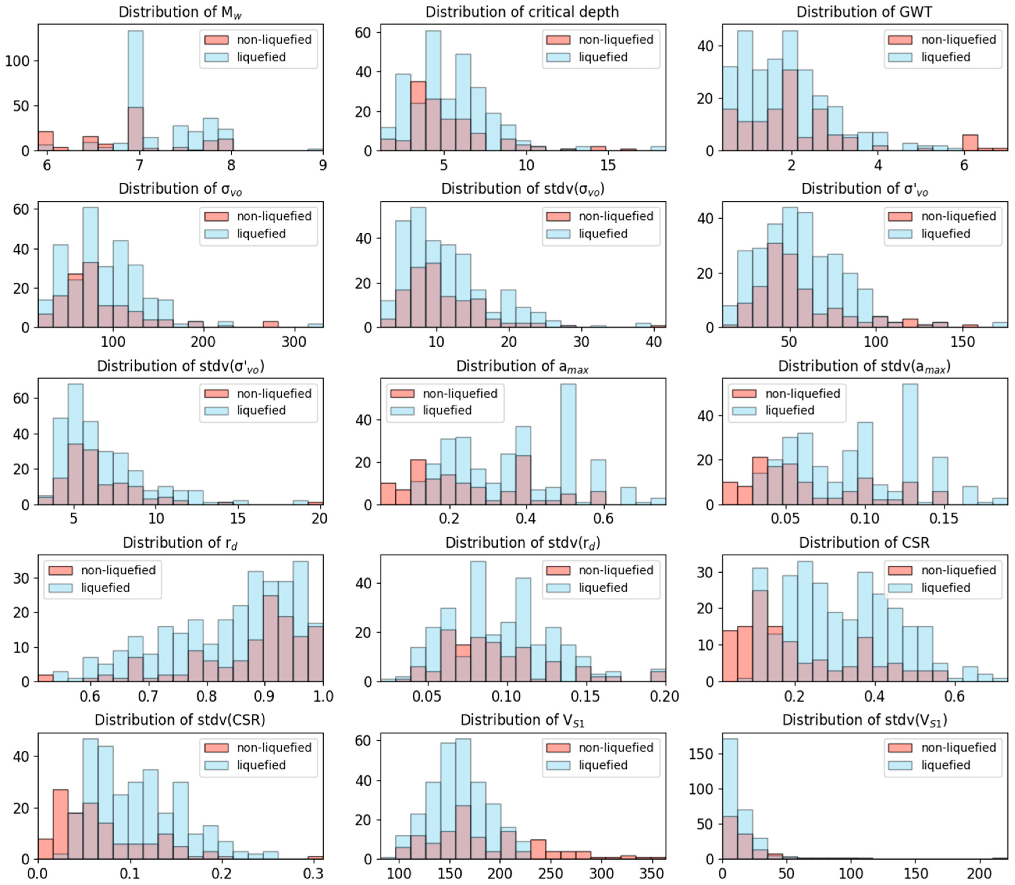
The dataset used in this study was compiled by Kayen, Moss [24] and includes normalized shear wave velocity $\left(V_{S1}\right)$ data from seismic regions across China, Japan, Taiwan, Greece, and the United States, collected over more than a decade. The original study focused on the probabilistic assessment of liquefaction using $V_{S1}$ data. The dataset consists of 415 data points from 301 sites, with each site characterized by 15 features critical to liquefaction potential. These features include earthquake moment magnitude ($M_w$), critical depth, the groundwater table depth (GWT), total vertical overburden stress (${\sigma }_{vo}$), effective vertical overburden stress (${\sigma }_{vo}^{\prime }$), peak horizontal ground acceleration at the surface ($a_{max}$), shear stress reduction coefficient ($r_d$), uniform cyclic stress ratio (CSR), and normalized shear wave velocity ($V_{S1}$). While the dataset covers a broad range of geotechnical parameters, it is important to note the absence of some key variables, such as fine content and soil type, which are often crucial in comprehensive liquefaction assessment. Each data point is paired with a binary target variable, indicating liquefaction occurrence, where “0” denotes non-liquefied and “1” denotes liquefied cases. An inspection of the dataset revealed no missing data, eliminating the need of data cleaning. However, the dataset is imbalanced, with 128 negative (non-liquefied) and 287 positive cases, as illustrated in Figure 1. The feature distribution across the liquefied and non-liquefied classes shows a skewed normal distribution for most features, as depicted in the histogram (Figure 1).

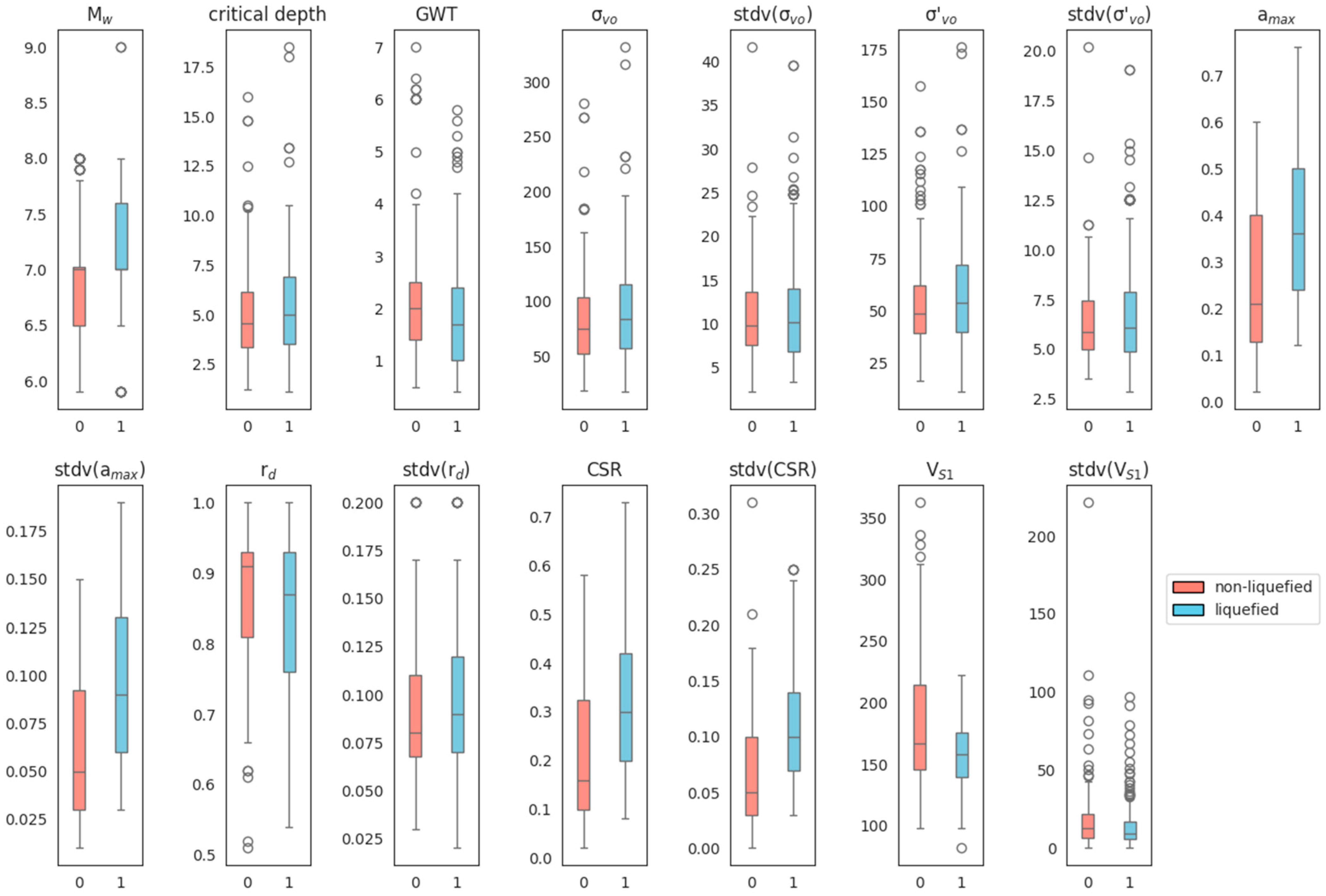
Further insights into the feature distribution are provided in the box plot in Figure 2, where the interquartile range for each feature is shown for both liquefied and non-liquefied classes. The median values are clearly marked within each box. The whiskers indicate the range relative to interquartile, and any outliers are marked separately by circles. Most data points fall within the interquartile and whisker ranges, suggesting that the data is well-distributed and does not require feature scaling.

2.2. Data Preprocessing

This study focuses on binary classification tasks using the dataset described earlier. Given the relatively modest size of the dataset, it is essential to maximize its utilization while minimizing bias to ensure robust model training and evaluation. To achieve this, cross-validation (CV) techniques were implemented. CV is widely used method that divides the dataset into multiple subsets (or folds), allowing the model to be trained on different combinations of these subsets and tested on the remaining data. This iterative process provides reliable performance estimates and reduces the likelihood of model performance being overly dependent on a single train-test split [25].

A 5-fold stratified CV technique was employed in this study, generating five distinct dataset splits. In each iteration, one subset was designated as the testing set, resulting in a train-test ratio of 80–20, where 80% of the data was used for training and 20% for testing. Importantly, stratification was applied to preserve the original dataset’s class distribution across all folds, preventing any additional data imbalance that might skew the results.

2.3. Classifiers

In this study, several widely used machine learning classifiers were employed, each representing different predictive approaches, including linear, non-parametric, and tree-based. In addition, common ensemble methods were also incorporated, both as base models and for comparison purposes. A brief introduction of each classifier and its respective objective function is provided in

Table 1. The classifiers used in this study with the short descriptions.

Classifiers	Descriptions
Logistic Regression (LR)	linear classification algorithm; predicts the probability of an instance belonging to a certain class using the logistic (sigmoid) function; operates under the assumption that the log-odds of the target variable being in a particular class is a linear combination of the input features [26].
Support Vector Classifier (SVC)	part of the Support Vector Machine family; can be linear or nonlinear depending on the kernel parameter; seeks to find the optimal hyperplane that best separates different classes in the input data by maximizing the margin between classes [27].
K-Nearest Neighbors (KNN)	non-parametric classification algorithm; classifies instances based on the majority class of nearest neighbors in the feature space; uses a distance metric such as Euclidean distance [28].
Gaussian Naive Bayes (GNB)	probabilistic classifier based on Bayes’ theorem; assumes features are independent and normally distributed; simplifies the calculation process and is suitable for features with continuous values [29].
Ridge Classifier (RC)	linear classification algorithm; incorporates L2 regularization to penalize large coefficients and prevent overfitting; useful for handling multicollinearity and improving model generalization [30].
Decision Tree Classifier (DT)	non-parametric, tree-based classification algorithm; recursively splits the input space into regions based on feature values, selecting the feature that best separates the data; maximizes information gain or minimizes impurity measures like Gini impurity or entropy [31].
Random Forest Classifier (RF)	ensemble learning algorithm with decision trees; combines multiple decision trees to improve accuracy and reduce overfitting; builds a forest of decision trees by training each tree on a random subset of features and instances, making predictions by aggregating the individual trees’ predictions [32].
Bagging Classifier (BC)	ensemble learning algorithm with decision trees; builds multiple base classifiers using bootstrapped samples of the training data, combining their predictions through averaging or voting to reduce variance and improve accuracy [33]; by default, the base estimator for the BC in the “scikit-learn” library is a DT classifier.
Gradient Boosting Classifier (GB)	ensemble learning algorithm with decision trees; combines boosting and gradient descent techniques builds decision trees subsequentially, with each tree correcting errors of previous ones, optimizing a differentiable loss function using gradient descent, and aggregating predictions weighted by a learning rate [34].

, highlighting the diversity of algorithms used in this study.

3. Methods

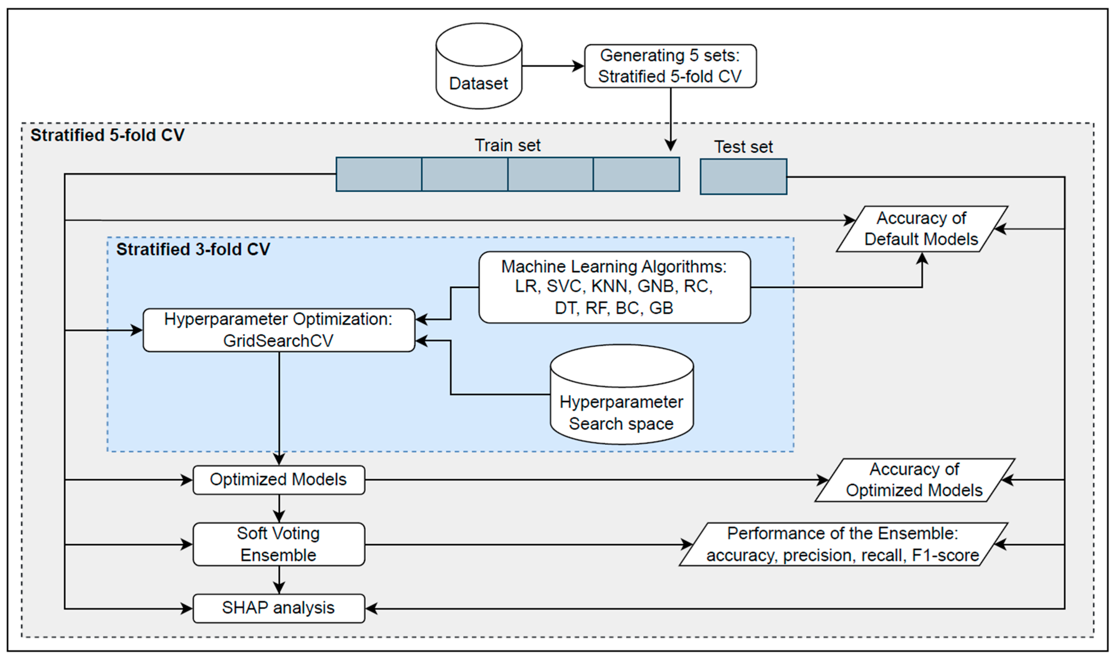
This section describes the methodology used for model evaluation, hyperparameter optimization, ensemble learning, and feature importance analysis using SHAP scores. The detailed workflow is illustrated in Figure 3. A 5-fold stratified CV was applied throughout the entire study to ensure consistent and unbiased performance estimation across all stages [35]. Stratification maintained the original class distribution in each fold, while the outer 5-fold CV provided reliable estimates of generalization performance. Within each outer fold, a nested 3-fold GridSearchCV was used during hyperparameter optimization of the base models.

Given the class imbalance in the dataset (128 non-liquefied and 287 liquefied cases) and the importance of minimizing false negatives in liquefaction risk detection, recall was adopted as the primary evaluation metric for model selection and ensemble weighting. This approach ensures that models are more sensitive to correctly identifying liquefied instances, which is critical for safety-oriented prediction tasks.

3.1. Dataset Correlation

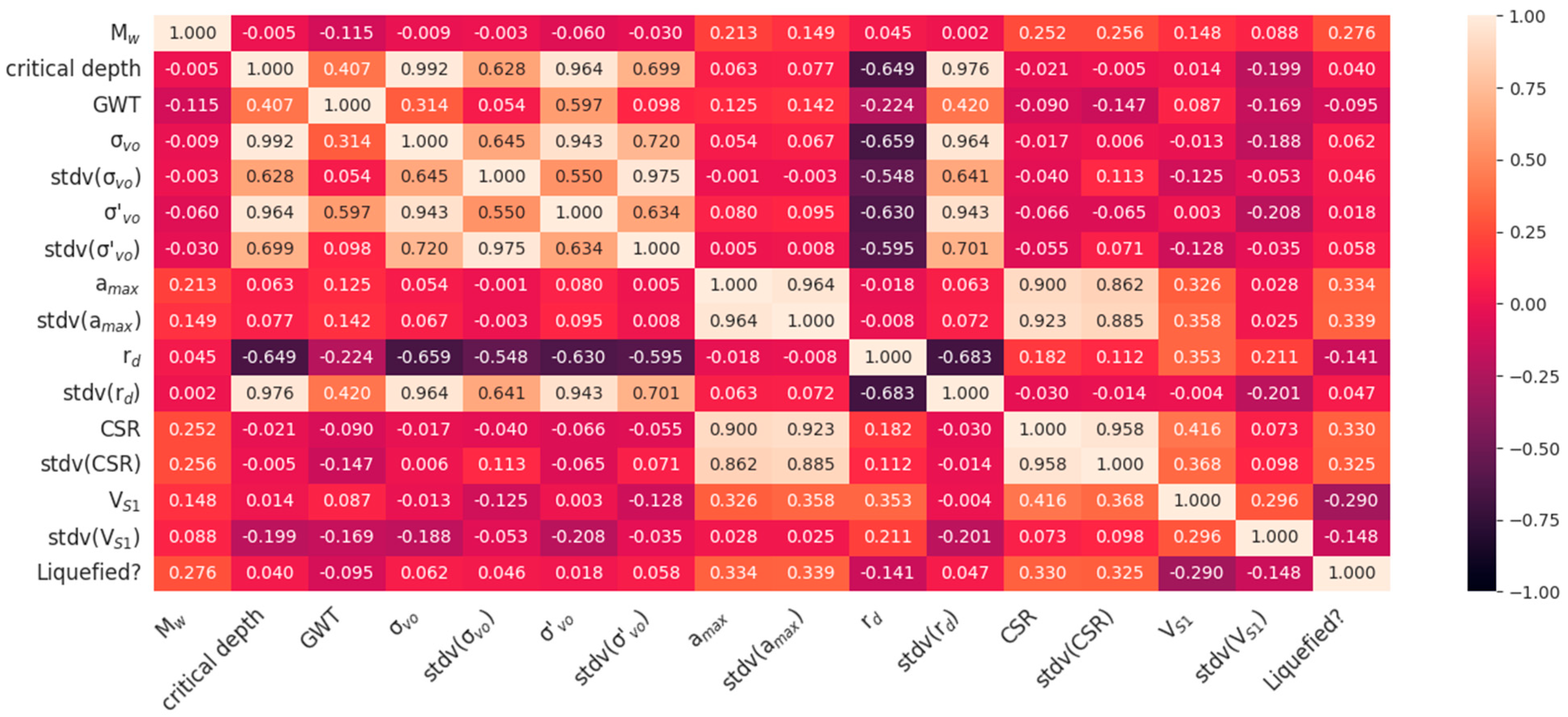
A correlation heatmap was generated to visualize the relationships among geotechnical input variables and the target liquefaction outcome. Each cell represents the Pearson correlation coefficient (r), calculated as:

$$r={\displaystyle \frac{\sum \left(x_i-\overline{x}\right)\left(y_i-\overline{y}\right)}{\sqrt{\sum {\left(x_i-\overline{x}\right)}^2\sum {\left(y_i-\overline{y}\right)}^2}}}$$

where $x_i$ and $y_i$ are sample values, and $\overline{x}$ and $\overline{y}$ are sample means. The coefficient ranges from −1 (strong negative correlation) to 1 (strong positive correlation), and coefficients close to 0 suggest little to no linear relationship. Identifying these relationships helps detect multicollinearity and support later SHAP-based feature interpretation by revealing linear dependencies between key input variables and liquefaction susceptibility.

3.2. Model Performance Metrics

Model performance was evaluated using several key metrics: accuracy, precision, recall, F1-score. Accuracy provides an overall measure of correct predictions but can be misleading for imbalanced datasets. Precision quantifies the reliability of liquefaction predictions by penalizing false alarms, whereas recall, the primary metric in this study, measures the model’s ability to correctly identify all liquefied cases—a critical factor for risk mitigation. The F1-score, balances precision and recall, and is informative under class imbalance. Additional evaluation tools, such as precision-recall (PR) and receiver operating characteristic (ROC) curves, as well as confusion matrices, were used to visualize performance trade-offs and prediction stability across cross-validation folds.

3.3. Hyperparameter Optimization

Hyperparameter optimization was performed using GridSearchCV with a 3-fold stratified CV nested within an outer 5-fold CV framework. This nested approach ensures unbiased model evaluation by separating the hyperparameter tuning process from performance estimation. The selection criterion for all models was based on recall score, reflecting the study’s focus on accurately identifying liquefied cases and minimizing false negatives.

A wide range of hyperparameter values were used to capture a broad spectrum from underfitting to overfitting behavior of each ML model. The predefined hyperparameter spaces (

Table 2. Hyperparameter optimization search space.

Classifier	Hyperparameter	Search Space
LR	penalty	L1, L2
	C	0.1, 1, 10, 100
SVC	kernel	linear, rbf
	C	0.1, 0.2, 0.5, 1, 2, 5, 10, 100, 1000
	gamma	0.001, 0.002, 0.005, 0.01, 0.02, 0.05, 0.1, 1, 10
KNN	n_neighbors	1, 2, 3, 4, 5, 6, 7, 8, 9, 10
	weights	uniform, distance
	algorithm	auto, ball_tree, kd_tree, brute
GNB	var_smoothing	1 × 10−6, 1 × 10−7, 1 × 10−8, 1 × 10−9, 1 × 10−10
RC	alpha	0.1, 0.2, 0.3, 0.4, 0.5, 0.6, 0.7, 0.8, 0.9, 1.0
	tol	1 × 10−3, 1 × 10−4, 1 × 10−5
DT	criterion	gini, entropy, log_loss
	max_depth	3, 5, 7, 10, 20, 50, 100
RF	max_features	3, 5, 7, 10, 20, 50
	max_depth	3, 5, 7, 10, 20, 50, 100
BC	max_features	0.1, 0.2, 0.3, 0.4, 0.5, 0.6, 0.7, 0.8, 0.9, 1.0
	max_samples	0.1, 0.2, 0.3, 0.4, 0.5, 0.6, 0.7, 0.8, 0.9, 1.0
GB	learning_rate	0.01, 0.1, 0.2, 0.5
	max_depth	3, 5, 8
	subsample	0.8, 0.9, 0.95, 1

Symbols: C—regularization strength; γ\gammaγ—kernel coefficient; α\alphaα—regularization term; tol—convergence tolerance.

) were determined based on literature review [36], empirical tuning [37], and domain-specific considerations [38]. In particular, the parameter intervals were guided by (i) ranges frequently adopted in previous studies using comparable classifiers, (ii) theoretical scales ensuring adequate model regularization and kernel sensitivity, and (iii) exploratory experiments on a subset of the training data to confirm effective coverage between underfitting and overfitting regions. For example, in the Support Vector Classifier, the search space for the kernel coefficient γ (0.001–10) and the regularization parameter C (0.1–1000) follows the logarithmic grid range commonly recommended in prior optimization studies [36,37] and is consistent with the scales empirically validated in recent domain-specific applications to liquefaction prediction [38].

Recall was used as the optimization metric during GridSearchCV, given the unbalanced nature of the dataset and to avoid false negatives. This combination of nested CV and systematic parameter search ensured robust and generalizable model performance.

3.4. Voting Ensemble

A Voting Ensemble technique was employed to combine predictions from multiple base models, aiming to improve the overall predictive performance. By aggregating the outputs of different base models, the ensemble model captures diverse patterns in the data and mitigates the limitations of individual classifiers.

The ensemble was constructed using a soft voting strategy, where base model probabilities were weighted by their normalized recall scores in each fold of 5-fold CV split after optimization. This approach provides more nuanced decisions than hard voting, while also enabling probabilistic predictions of liquefaction risk. The weight $w_i$ for model i in each fold was calculated as:

$$w_i={\displaystyle \frac{R_i}{{\sum }_j{R}_j}}$$

where $R_i$ denotes the recall of i-th optimized classifier in a fold. This weighting ensures that each ensemble reflects the relative performance of its base models without information leakage across folds. To verify that this weighting scheme did not bias performance, a sensitivity analysis (Table S1) comparing equal, accuracy-based, and recall-based weighting was conducted.

3.5. Feature Importance Analysis (SHAP)

To assess the contribution of individual features to liquefaction susceptibility, we employed SHAP, a method designed to explain the predictions of complex ML models [23]. SHAP calculates the marginal contribution of each feature value to a model’s prediction, using cooperative game theory’s Shapley values. This technique assigns importance scores to features by analyzing their impact on the prediction, facilitating the interpretation of non-linear models.

In this study, SHAP values were computed for each fold of the cross-validation using the trained ensemble model. These values were then aggregated to provide a comprehensive view of feature importance across all folds. Visualizations such as bar plots and beeswarm plots were generated to describe the relative importance of each feature in predicting liquefaction susceptibility. The combination of cross-validation, ensemble learning, and SHAP analysis enabled a thorough understanding of the feature contributions, enhancing both the interpretability and reliability of the predictive models.

4. Results and Discussion

4.1. Dataset Correlation

Figure 4 presents the correlation heatmap, which illustrates the relationships between the input features and the liquefaction occurrence. The analysis reveals that only a few features exhibit significant correlations with the target variable. The highest correlations were observed with the features: $a_{max}$ (0.334), CSR (0.330), $V_{S1}$ (−0.290), and $M_w$ (0.276). Despite these values, the correlations with liquefaction presence remain relatively low.

Several feature pairs displayed strong inter-correlations. For instance, critical depth demonstrated a high positive correlation with both total stress (0.992) and effective stress (0.964), suggesting that as these stresses increases, so does the critical depth for liquefaction susceptibility. Additionally, $a_{max}$ and CSR exhibited a strong positive correlation (0.900), indicating that higher seismic accelerations are associated with higher cyclic stress ratios. Conversely, $r_d$ showed negative correlations with critical depth (−0.649), total stress (−0.659), and effective stress (−0.630), emphasizing the complex interplay between different geotechnical parameters and liquefaction potential. Further analysis using SHAP is expected to provide deeper insights into the role of each input in liquefaction prediction.

4.2. Base Models Performance

The performance of multiple ML classifiers was evaluated using a robust, two-layer stratified cross-validation (CV) framework, with recall adopted as the primary metric due to the class imbalance and the critical importance of correctly identifying liquefied instances. The examined classifiers included logistic regression (LR), support vector classifier (SVC), k-nearest neighbors (KNN), Gaussian naive Bayes (GNB), ridge classifier (RC), decision tree (DT), random forest (RF), bagging classifier (BC), and gradient boosting (GB).

Initial evaluations with 5-fold stratified CV (outer loop) were conducted using default hyperparameters to assess baseline generalization performance (

Table 3. Default base models performance.

Model	Accuracy (±stdv)		Precision (±stdv)		Recall (±stdv)		F1-Score (±stdv)
LR	82.65%	±3.20%	84.36%	±2.26%	91.98%	±2.38%	88.00%	±2.22%
SVC	86.75%	±2.95%	85.20%	±2.42%	97.91%	±1.30%	91.10%	±1.87%
KNN	81.69%	±2.79%	81.16%	±2.18%	95.83%	±2.58%	87.86%	±1.86%
GNB	78.31%	±5.00%	83.96%	±4.16%	85.00%	±3.84%	84.43%	±3.55%
RC	82.89%	±3.18%	82.93%	±1.84%	94.75%	±3.51%	88.43%	±2.26%
DT	86.02%	±3.62%	89.80%	±4.35%	90.25%	±1.76%	89.97%	±2.46%
RF	87.23%	±3.54%	87.53%	±2.55%	95.14%	±2.27%	91.17%	±2.35%
BC	89.16%	±5.70%	91.16%	±3.93%	93.39%	±4.28%	92.25%	±4.05%
GB	88.43%	±4.97%	88.63%	±2.52%	95.49%	±4.95%	91.91%	±3.58%

). Ensemble-based classifiers such as BC, GB, and RF, achieved the highest overall accuracy and recall though with higher variability, indicating some instability across folds. Notably, SVC and KNN demonstrated strong recall values (97.91% and 95.83%, respectively), emphasizing their ability to correctly detect liquefied cases even at the cost of lower precision. In contrast, GNB exhibited the weakest performance, likely due to its Gaussian assumptions being inconsistent with the actual feature distributions.

To further enhance model performance, hyperparameter optimization was performed using a nested 3-fold stratified GridSearchCV within each outer fold. This process improved the sensitivity of several models, as summarized in

Table 4. Optimized base model performance.

Model	Accuracy (±stdv)		Precision (±stdv)		Recall (±stdv)		F1-Score (±stdv)
LR	83.61%	±3.54%	83.70%	±2.13%	94.75%	±4.16%	88.85%	±2.61%
SVC	85.78%	±3.99%	86.32%	±2.58%	94.42%	±3.88%	90.16%	±2.79%
KNN	85.30%	±4.34%	84.86%	±4.56%	96.18%	±1.68%	90.11%	±2.77%
GNB	78.31%	±5.00%	83.96%	±4.16%	85.00%	±3.84%	84.43%	±3.55%
RC	82.41%	±3.62%	83.01%	±1.76%	93.72%	±4.06%	88.02%	±2.59%
DT	85.30%	±4.78%	86.60%	±5.53%	93.74%	±2.57%	89.91%	±2.96%
RF	87.71%	±5.67%	87.68%	±4.26%	95.82%	±3.57%	91.55%	±3.78%
BC	87.47%	±5.98%	89.43%	±4.59%	93.02%	±4.53%	91.15%	±4.10%
GB	88.92%	±5.46%	89.48%	±3.17%	95.14%	±4.67%	92.22%	±3.86%

. For example, KNN’s recall increased from 95.83% to 96.18%, after tuning the number of neighbors and distance metric, while DT’s recall rose by 3.5%. Ensemble methods such as GB and RF maintained consistently high recall after optimization, confirming their robustness. Overall, the optimized models demonstrated strong generalization in identifying positive (liquefied) instances, providing a solid basis for subsequent ensemble construction.

4.3. Voting Ensemble Performance

The final model employed in this study was a soft Voting Ensemble, excluding GNB due to its inferior individual performance. As shown in

Table 5. Voting Ensemble performance across each fold.

Fold	Accuracy	Precision	Recall	F1-Score
1	81.93%	84.13%	91.38%	87.60%
2	91.57%	90.48%	98.28%	94.21%
3	90.36%	90.16%	96.49%	93.22%
4	95.18%	93.44%	100.00%	96.61%
5	91.57%	89.06%	100.00%	94.21%
Mean	90.12%	89.45%	97.23%	93.17%
Stdv	4.53%	3.20%	3.20%	3.09%

, the ensemble consistently outperformed its base learners and other ensemble models. It achieved a mean accuracy of 90.12%, precision of 89.45%, recall of 97.23%, and F1-score of 93.17% across five folds.

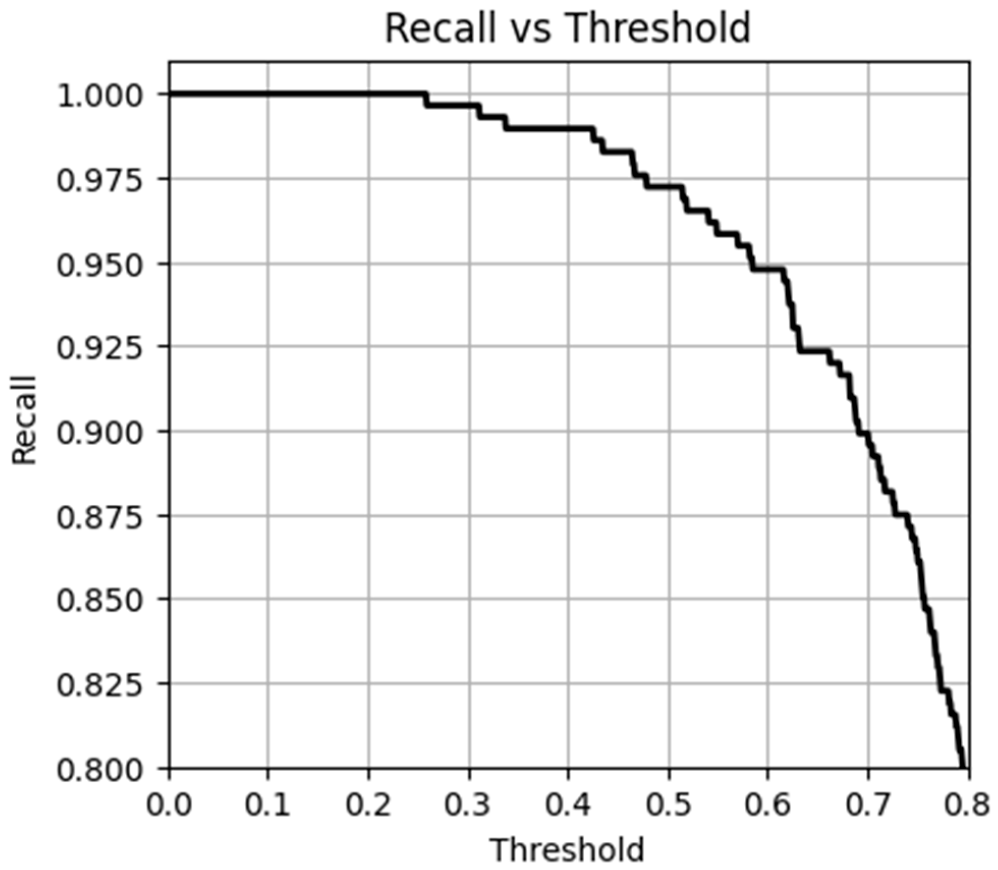
The Voting Ensemble utilized a soft voting strategy, aggregating predicted probability from base models, with a threshold of 0.5 for liquefaction. Figure 5 illustrates that lowering the threshold to 0.25 further increases recall to 100%, demonstrating the model’s sensitivity control, which is particularly valuable in hazard prediction tasks.

The Voting Ensemble demonstrated robustness across all five folds, with low standard deviations in accuracy and recall, indicating reliable generalization and limited sensitivity to data partitioning. Moreover, a sensitivity analysis comparing equal, accuracy-based, and recall-based weighting strategies (Table S1) confirmed that performance metrics remained effectively unchanged across weighting schemes. This suggests that the ensemble’s stability stems from consistent agreement among base classifiers rather than dependence on specific weighting. Nonetheless, recall-based weighting was retained in the final model to prioritize correct identification of liquefaction cases, ensuring maximal sensitivity without increasing false positives, while the robustness check demonstrates that this choice does not compromise overall ensemble stability.

4.4. Comparison with Other Studies

A comparative assessment was conducted to position the proposed Voting Ensemble against previous ML-based liquefaction prediction studies. Only studies employing binary classification approaches were included, while those focusing on regression-based estimation of the factor of safety [22,39], were excluded due to incompatible evaluation metrics.

Table 6. Liquefaction classification results from different studies.

Research Paper	Dataset (liq.:non-liq.)	Dataset Type	# of Inputs	Algorithm	Accuracy	Recall
This study	415 (287:128)	$V_{S1}$	15	Voting Ensemble	90.12%	97.23%
[40]	296 (159:137)	DPT	5	LightGBM	83.33%	83.33%
[21]	273 (87:186)	CPT	7	DT	89%	77%
				RF	77%	80%
[20]	226 (133:93)	CPT	7	CCF	96.42%	96.43%
[19]	411 (287:124)	$V_{S1}$	9	ANN + NSGA-II	90.51%	89.55%
				ANN + MOSOS	92.94%	92.68%
[41]	226 (133:93)	CPT	6	RF	99.48%	N/A
[2]	226 (133:93)	CPT	6	SVM	97%	N/A
[12]	85 (42:43)	SPT	8	ANN	92%	N/A

CCF—canonical correlation forest; DPT—dynamic penetration test; LightGBM—light gradient boosting machine; MOSOS—multi-objective symbiotic organisms search; NSGA—non-dominated sorting genetic algorithm; SVM—support vector machine.

summarizes the datasets, model types, and reported results from comparable studies. Das, Mohanty [19] emphasized that conventional accuracy may be mis-leading in unbalanced datasets, suggesting instead the use of the geometric mean of class accuracies. In this study, however, accuracy and recall were prioritized—accuracy reflecting overall performance, and recall capturing the model’s ability to correctly identify liquefied sites.

The proposed Voting Ensemble achieved an accuracy of 90.12% and a recall of 97.23%, demonstrating strong capability in identifying liquefied cases. High recall is particularly valuable in hazard assessment, as missing true liquefaction instances (false negatives) can lead to unsafe design conclusions. When compared with the canonical correlation forest (CCF) of Demir and Sahin [20] and the ANN–MOSOS hybrid of Das, Mohanty [19], the Voting Ensemble achieved slightly lower accuracy but higher sensitivity, implying a more balanced trade-off between precision and generalization.

The exceptionally high accuracies reported for RF [41] and SVM [2] (>97%) could be attributed to factors such as data noise, overfitting, and smaller datasets. Notably, both RF and SVM were included as base learners in the Voting Ensemble; their integration with Gradient Boosting and Bagging Classifier reduced individual model bias and improved overall stability across folds.

While empirical frameworks such as the liquefaction triggering model of Kayen, Moss [24] remain valuable for deterministic assessment, they are constrained by specific site conditions and simplified assumptions about soil behavior. The proposed ML ensemble provides a complementary, data-driven alternative that captures nonlinear interactions among geotechnical and seismic variables without imposing predefined functional forms. The Voting Ensemble therefore complements, rather than replaces, traditional empirical methods—offering a robust, interpretable, and statistically validated alternative for liquefaction assessment through cross-validation, hyperparameter optimization, and SHAP-based feature analysis.

4.5. Confusion Matrix

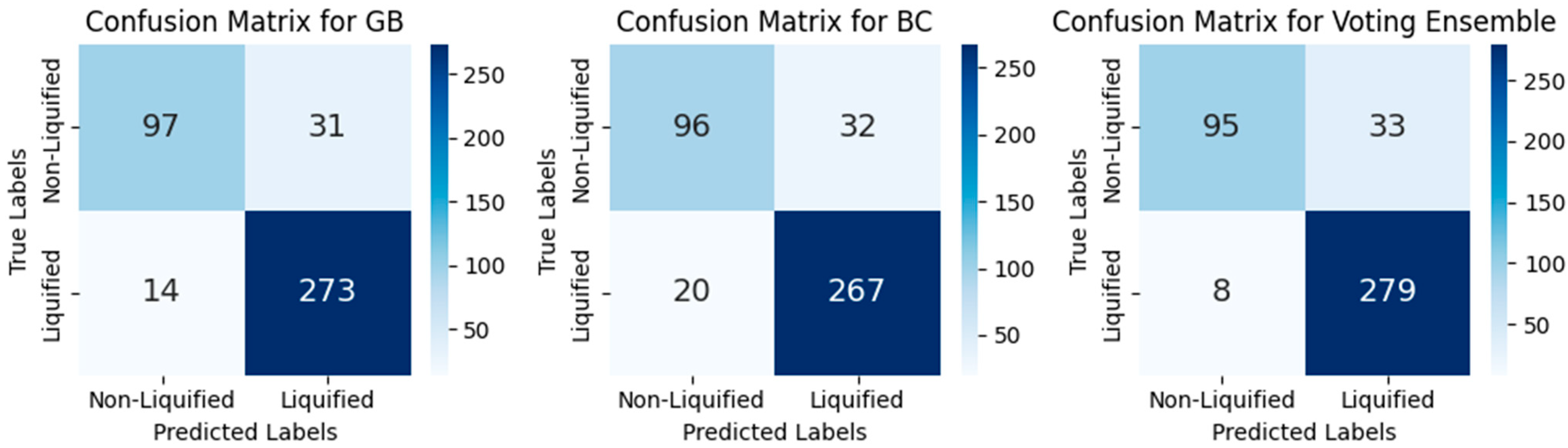
Figure 6 presents the classification performance of the Voting Ensemble alongside two commonly used ensemble models (GB and BC) for “non-liquified” and “liquified” instances. The confusion matrices were generated by aggregating predictions across all CV folds. As expected, all models showed higher misclassification rates for “non-liquified” instances due to the inherent class imbalance in the dataset.

In liquefaction risk prediction, the key objective is to accurately identify actual liquefied cases (true positives, TP), while minimizing false negatives (FN), as missing liquefaction-prone sites could have severe implications for safety. Both GB and BC achieved strong detection performance; however, the Voting Ensemble demonstrated superior capability by correctly identifying 279 liquefied cases and reducing FN to only 8.

These results highlight the robustness of the Voting Ensemble in capturing liquefaction-prone sites, while maintaining balanced performance across both classes. The confusion matrix analysis confirms that the ensemble framework effectively reduces misclassification risk compared to other ensemble models.

4.6. ROC and PR Curves

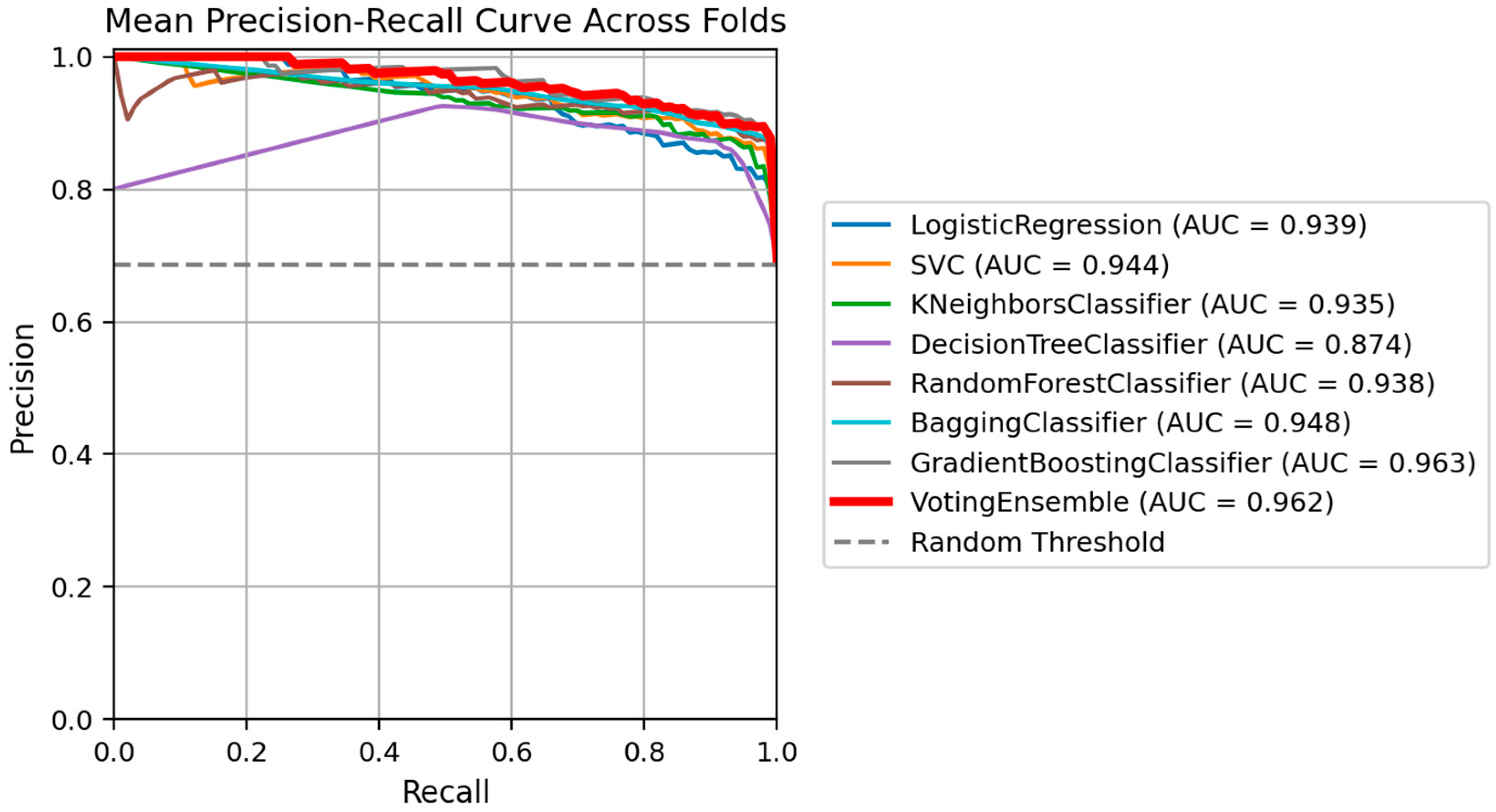
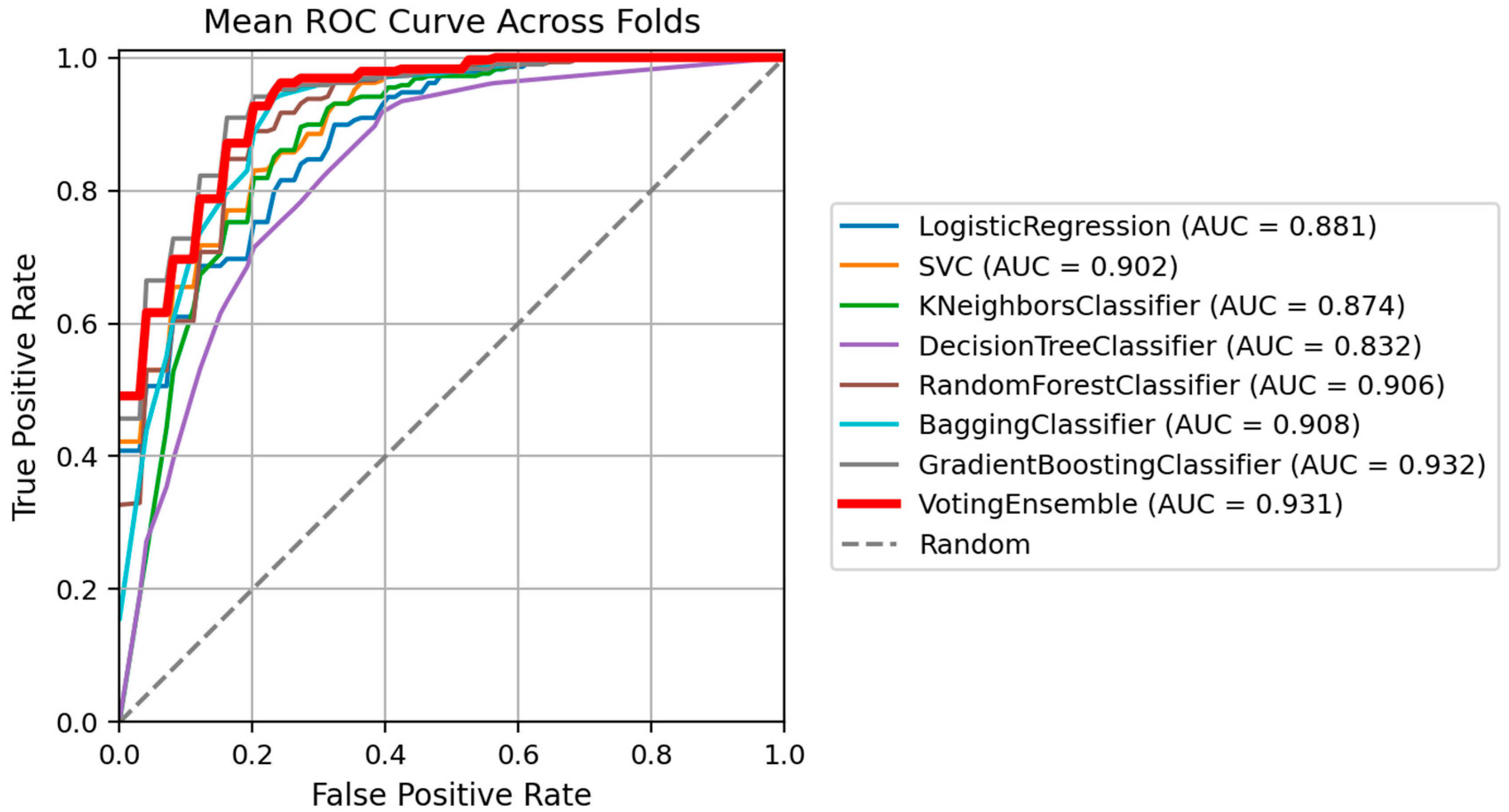
The ROC and PR curves provide a comprehensive evaluation of model performance across various decision thresholds. Figure 7 and Figure 8 present the mean ROC and PR curves averaged over all CV folds. GB model achieved the highest overall discrimination ability, with ROC AUC and PR AUC values of 0.932 and 0.963, respectively. The Voting Ensemble followed closely with nearly identical scores: ROC AUC = 0.931 and PR AUC = 0.962; demonstrating highly competitive performance. Other strong performers included BC (ROC AUC = 0.908, PR AUC = 0.948) and RF (ROC AUC = 0.906, PR AUC = 0.938), while LR and SVC showed balanced and stable results with ROC AUCs above 0.88.

Despite Gradient Boosting’s marginally higher AUCs, the Voting Ensemble consistently achieved better accuracy, recall, and F1-scores across individual cross-validation folds. This apparent discrepancy highlights the nuanced difference between ranking-based metrics (AUC) and threshold-based metrics (accuracy, recall, F1). AUC reflects the model’s ability to rank liquefaction and non-liquefaction cases correctly across all decision thresholds, while recall and F1 depend on a fixed threshold (typically 0.5). The Voting Ensemble’s probability averaging across diverse base classifiers smooths out overconfident predictions and reduces variance, yielding more balanced and reliable classification outcomes.

Therefore, although Gradient Boosting displayed a slightly superior theoretical discrimination capacity, the Voting Ensemble demonstrated more consistent practical performance, especially in identifying liquefied cases—a key objective in risk-sensitive applications. This combination of high AUC stability and superior threshold-level metrics underscores the ensemble’s robustness and suitability for operational liquefaction risk prediction.

4.7. SHAP Analysis

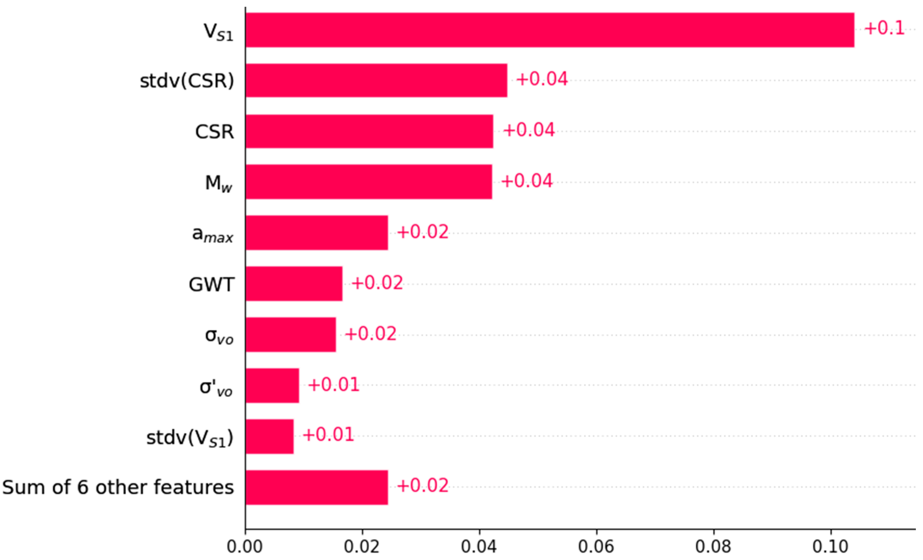
SHAP analysis was conducted to provide an interpretable understanding of how individual features influenced the predictions of the Voting Ensemble for liquefaction susceptibility. Figure 9 depicts the feature importance, showing the mean absolute SHAP values for each variable. The normalized shear wave velocity ($V_{S1}$) had the highest impact, with a substantial gap compared to other features, contributing a SHAP value of 0.1. This finding aligns with well-established geotechnical theory, as $V_{S1}$ reflects small-strain shear stiffness—a fundamental indicator of soil rigidity and its ability to resist cyclic shear stress during earthquakes. Previous studies also highlight $V_{S1}$ as a key proxy for liquefaction resistance through its correlation with CRR [10,24]. Thus, the model’s emphasis on $V_{S1}$ is consistent with established physical understanding.

The next most influential features were related to seismic loading, including the standard deviation of CSR (0.04), CSR (0.04), $M_w$ (0.04), and $a_{max}$ (0.02). Their high SHAP contributions are physically consistent since CSR and $M_W$ jointly characterize the intensity and duration of cyclic loading, which directly control pore pressure buildup and soil response. This reflects Voting Ensemble model’s ability to capture magnitude scaling effects in liquefaction analysis.

Additional critical factors identified in the SHAP analysis include GWT, ${\sigma }_{vo}$ and ${\sigma }_{vo}^{\prime }$ These variables govern effective stress and drainage conditions. These are the key mechanisms influencing pore pressure development, which play a significant role in liquefaction. Their moderate SHAP values confirm the model’s consistency with geotechnical theory.

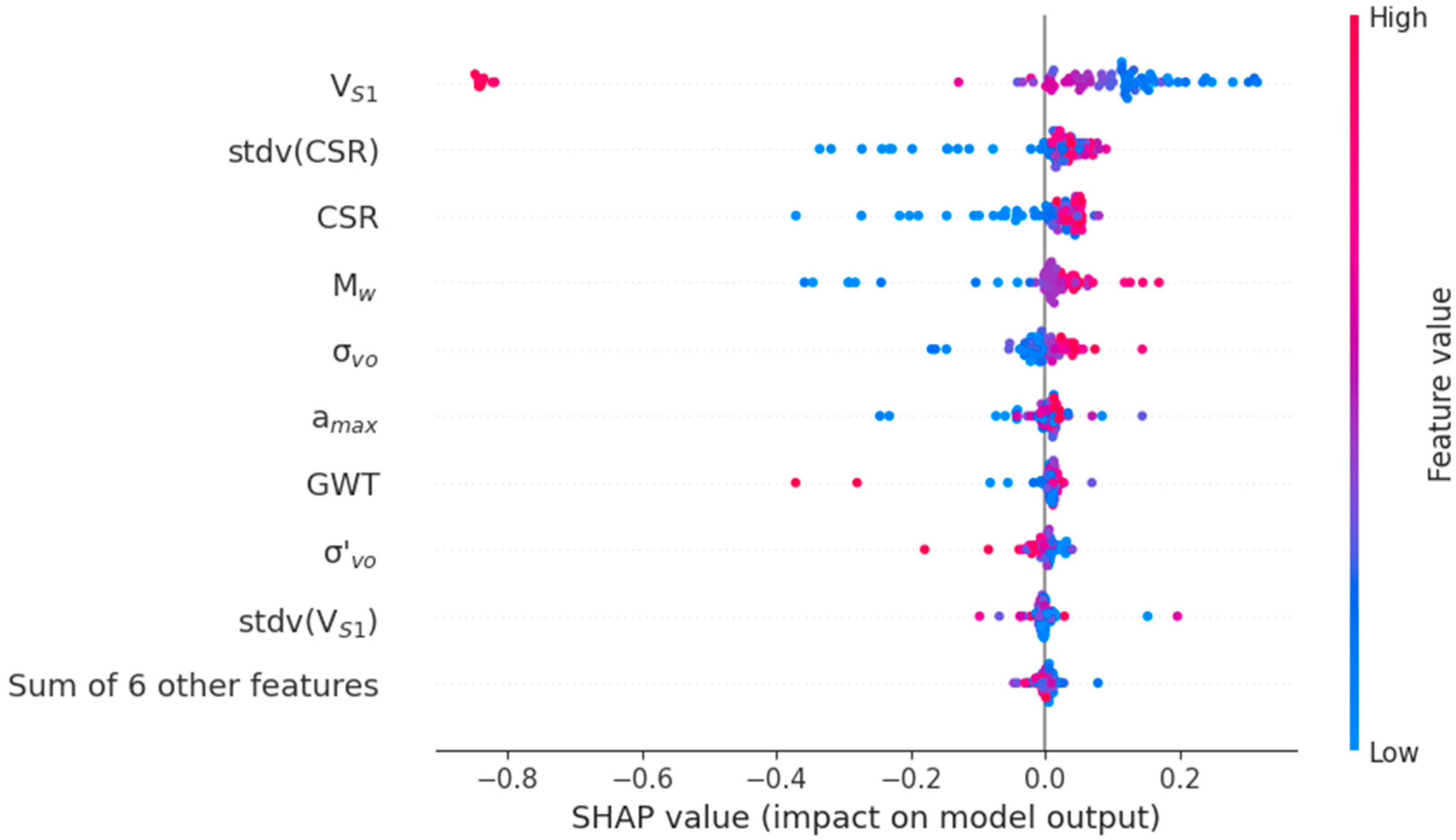
Further insights were derived from the SHAP beeswarm plot, illustrated in Figure 10, which reveals a sample-level perspective of how each feature influences individual predictions within the Voting Ensemble model. Each point represents a data instance, with the x-axis showing SHAP values and its color indicating the corresponding feature magnitude.

While most variables displayed dispersed SHAP distributions, $V_{S1}$ distinctly dominated with a strong, directionally consistent pattern. High $V_{S1}$ values clustered around negative SHAP impacts (≈−0.8), reflecting reduced liquefaction probability, whereas low $V_{S1}$ values corresponded to positive SHAP impacts (≈0.1–0.3), indicating elevated susceptibility. This clear inverse relationship aligns with geotechnical principles, as shear wave velocity is an indirect indicator of liquefaction resistance. The consistency between the SHAP trend and the physical behavior of soils reinforces the model’s reliability and its adherence to established liquefaction theory.

Other features, such as std(CSR), CSR, $M_w$ and ${\sigma }_{vo}$ exhibited subtler yet meaningful patterns, with lower values generally contributed positively to liquefaction prediction. Although these parameters did not exhibit strong linear correlations in the preliminary heatmap analysis, SHAP revealed their combined and nonlinear effects, emphasizing the model’s capability to capture interaction terms often simplified or parameterized in empirical formulations. Interestingly, $a_{max}$ which initially showed high correlation, demonstrated limited attribution across both low and high magnitudes, indicating that feature interdependencies attenuate its standalone contribution. Overall, the beeswarm visualization confirms that the ensemble model not only ranks features correctly but also mirrors real geotechnical mechanisms, bridging the gap between data-driven inference and soil behavior understanding.

5. Conclusions

This study demonstrates significant advancements in the predictive modeling of soil liquefaction by integrating hyperparameter optimization, ensemble modeling, and SHAP-based interpretability within a robust stratified 5-fold cross-validation framework. Hyperparameter tuning enhanced the performance of individual classifiers, with Gradient Boosting (GB) and Bagging classifier (BC) emerging as the strongest base models. When combined through a soft Voting Ensemble, their collective performance matched or surpassed that of the best standalone models across multiple metrics, including accuracy, recall, F1-score, and AUC values from both ROC and PR curves.

SHAP analysis provided critical insights into the model’s interpretability, identifying normalized shear wave velocity ($V_{s1}$) as the most critical parameter, followed by CSR and $M_W$ The Voting Ensemble’s decision logic aligns closely with geotechnical principles, confirming that the proposed ML framework captures meaningful physical relationships.

Overall, the Voting Ensemble demonstrated a balanced trade-off between accuracy and robustness, which are essential for practical implementation in geotechnical engineering. Future research should extend this framework by incorporating other types of ensemble and neural network architectures, such as stacked ensembles and hybrid deep learning models, to further improve the performance of liquefaction prediction systems.

References

1. Youd, T.L.; Idriss, I.M. Liquefaction Resistance of Soils: Summary Report from the 1996 NCEER and 1998 NCEER/NSF Workshops on Evaluation of Liquefaction Resistance of Soils. J. Geotech. Geoenviron. Eng. 2001, 127, 297–313. [Google Scholar] [CrossRef]
2. Goh, A.T.C.; Goh, S.H. Support vector machines: Their use in geotechnical engineering as illustrated using seismic liquefaction data. Comput. Geotech. 2007, 34, 410–421. [Google Scholar] [CrossRef]
3. Ishac, M.F.; Heidebrecht, A.C. Energy dissipation and seismic liquefaction in sands. Earthq. Eng. Struct. Dyn. 1982, 10, 59–68. [Google Scholar] [CrossRef]
4. Seed, H.B.; Idriss, I.M. Analysis of Soil Liquefaction: Niigata Earthquake. J. Soil Mech. Found. Div. 1967, 93, 83–108. [Google Scholar] [CrossRef]
5. Dobry, R.; Abdoun, T. Cyclic Shear Strain Needed for Liquefaction Triggering and Assessment of Overburden Pressure Factor Kσ. J. Geotech. Geoenvironmental Eng. 2015, 141, 04015047. [Google Scholar] [CrossRef]
6. Robertson, P.K.; Woeller, D.J.; Finn, W.D.L. Seismic cone penetration test for evaluating liquefaction potential under cyclic loading. Can. Geotech. J. 1992, 29, 686–695. [Google Scholar] [CrossRef]
7. Seed, H.B.; Idriss, I.M. Simplified Procedure for Evaluating Soil Liquefaction Potential. J. Soil Mech. Found. Div. 1971, 97, 1249–1273. [Google Scholar] [CrossRef]
8. Choi, D.-H.; Kwon, T.-H.; Ko, K.-W. Centrifuge Modeling of Soil Liquefaction Triggering: 2017 Pohang Earthquake. KSCE J. Civ. Eng. 2024, 28, 3176–3191. [Google Scholar] [CrossRef]
9. Ko, K.-W.; Lee, S.-B.; Oh, T.-S.; Kim, N.-R.; Kim, J.-H. Performance Evaluation of Sieve and Curtain Pluviators for Reconstituted Sand Specimen in Model Box. KSCE J. Civ. Eng. 2024, 28, 5452–5463. [Google Scholar] [CrossRef]
10. Andrus, R.D.; Stokoe II, K.H. Liquefaction Resistance of Soils from Shear-Wave Velocity. J. Geotech. Geoenvironmental Eng. 2000, 126, 1015–1025. [Google Scholar] [CrossRef]
11. Moon, S.W.; Mukhtarkhan, D.; Khamitov, R.; Abdialim, S.; Shokbarov, Y.; Kim, J.; Ku, T. Liquefaction Assessment using Surface Waves in Kazakhstan. In Proceedings of the 18th World Conference on Earthquake Engineering (WCEE2024), Milan, Italy, 30 June–5 July 2024. [Google Scholar]
12. Goh, A.T.C. Seismic Liquefaction Potential Assessed by Neural Networks. J. Geotech. Eng. 1994, 120, 1467–1480. [Google Scholar] [CrossRef]
13. Shao, W.; Yue, W.; Zhang, Y.; Zhou, T.; Zhang, Y.; Dang, Y.; Wang, H.; Feng, X.; Chao, Z. The Application of Machine Learning Techniques in Geotechnical Engineering: A Review and Comparison. Mathematics 2023, 11, 3976. [Google Scholar] [CrossRef]
14. Fattah, E.A.; Ali, H.E.A.; Ebid, A.M. Prediction of Soil Liquefaction Using Genetic Programming. In Proceedings of the III Middel East Regional Conference on Civil Engineering Technology and III International Symposium on Environmental Hydrology, Dubai, United Arab Emirates, 29–30 September 2025. [Google Scholar]
15. Pal, M. Support vector machines-based modelling of seismic liquefaction potential. Int. J. Numer. Anal. Methods Geomech. 2006, 30, 983–996. [Google Scholar] [CrossRef]
16. Hu, J.-L.; Tang, X.-W.; Qiu, J.-N. Assessment of seismic liquefaction potential based on Bayesian network constructed from domain knowledge and history data. Soil Dyn. Earthq. Eng. 2016, 89, 49–60. [Google Scholar] [CrossRef]
17. Hu, H.; Hu, X.; Gong, X. Predicting the strut forces of the steel supporting structure of deep excavation considering various factors by machine learning methods. Undergr. Space 2024, 18, 114–129. [Google Scholar] [CrossRef]
18. Jas, K.; Dodagoudar, G.R. Liquefaction Potential Assessment of Soils Using Machine Learning Techniques: A State-of-the-Art Review from 1994–2021. Int. J. Geomech. 2023, 23, 03123002. [Google Scholar] [CrossRef]
19. Das, S.K.; Mohanty, R.; Mohanty, M.; Mahamaya, M. Multi-objective feature selection (MOFS) algorithms for prediction of liquefaction susceptibility of soil based on in situ test methods. Nat. Hazards 2020, 103, 2371–2393. [Google Scholar] [CrossRef]
20. Demir, S.; Sahin, E.K. Comparison of tree-based machine learning algorithms for predicting liquefaction potential using canonical correlation forest, rotation forest, and random forest based on CPT data. Soil Dyn. Earthq. Eng. 2022, 154, 107130. [Google Scholar] [CrossRef]
21. Ozsagir, M.; Erden, C.; Bol, E.; Sert, S.; Özocak, A. Machine learning approaches for prediction of fine-grained soils liquefaction. Comput. Geotech. 2022, 152, 105014. [Google Scholar] [CrossRef]
22. Kurnaz, T.F.; Erden, C.; Kökçam, A.H.; Dağdeviren, U.; Demir, A.S. A hyper parameterized artificial neural network approach for prediction of the factor of safety against liquefaction. Eng. Geol. 2023, 319, 107109. [Google Scholar] [CrossRef]
23. Lundberg, S.M.; Lee, S.-I. A unified approach to interpreting model predictions. In Proceedings of the 31st International Conference on Neural Information Processing Systems, Long Beach, CA, USA, 2–6 December 2024; pp. 4768–4777. [Google Scholar]
24. Kayen, R.; Moss, R.E.S.; Thompson, E.M.; Seed, R.B.; Cetin, K.O.; Kiureghian, A.D.; Tanaka, Y.; Tokimatsu, K. Shear-Wave Velocity–Based Probabilistic and Deterministic Assessment of Seismic Soil Liquefaction Potential. J. Geotech. Geoenvironmental Eng. 2013, 139, 407–419. [Google Scholar] [CrossRef]
25. Kohavi, R. A study of cross-validation and bootstrap for accuracy estimation and model selection. In Proceedings of the 14th International Joint Conference on Artificial Intelligence—Volume 2, Montreal, QC, Canada, 20–25 August 1995; pp. 1137–1143. [Google Scholar]
26. Kleinbaum, D.G.; Klein, M. Logistic Regression, 3rd ed.; Springer: New York, NY, USA, 2010; p. 702. [Google Scholar] [CrossRef]
27. Cortes, C.; Vapnik, V. Support-vector networks. Mach. Learn. 1995, 20, 273–297. [Google Scholar] [CrossRef]
28. Cover, T.M.; Hart, P.E. Nearest Neighbor Pattern Classification. IEEE Trans. Inf. Theory 1967, 13, 21–27. [Google Scholar] [CrossRef]
29. Friedman, N.; Geiger, D.; Goldszmidt, M. Bayesian Network Classifiers. Mach. Learn. 1997, 29, 131–163. [Google Scholar] [CrossRef]
30. Hastie, T.; Tibshirani, R.; Friedman, J. The Elements of Statistical Learning, 2nd ed.; Springer: New York, NY, USA, 2009. [Google Scholar] [CrossRef]
31. Breiman, L.; Friedman, J.H.; Olshen, R.A.; Stone, C.J. Classification and Regression Trees, 1st ed.; Chapman and Hall/CRC: Boca Raton, FL, USA, 1984; p. 368. [Google Scholar] [CrossRef]
32. Breiman, L. Random Forests. Mach. Learn. 2001, 45, 5–32. [Google Scholar] [CrossRef]
33. Breiman, L. Bagging predictors. Mach. Learn. 1996, 24, 123–140. [Google Scholar] [CrossRef]
34. Friedman, J.H. Greedy function approximation: A gradient boosting machine. Ann. Stat. 2001, 29, 1189–1232. [Google Scholar] [CrossRef]
35. Varma, S.; Simon, R. Bias in error estimation when using cross-validation for model selection. BMC Bioinform. 2006, 7, 91. [Google Scholar] [CrossRef] [PubMed]
36. Yang, L.; Shami, A. On hyperparameter optimization of machine learning algorithms: Theory and practice. Neurocomputing 2020, 415, 295–316. [Google Scholar] [CrossRef]
37. Feurer, M.; Klein, A.; Eggensperger, K.; Springenberg, J.T.; Blum, M.; Hutter, F. Learning. In Automated Machine Learning: Methods, Systems, Challenges; Hutter, F., Kotthoff, L., Vanschoren, J., Eds.; Springer International Publishing: Cham, Switzerland, 2019; pp. 113–134. [Google Scholar] [CrossRef]
38. Şehmusoğlu, E.H.; Kurnaz, T.F.; Erden, C. Estimation of soil liquefaction using artificial intelligence techniques: An extended comparison between machine and deep learning approaches. Environ. Earth Sci. 2025, 84, 130. [Google Scholar] [CrossRef]
39. Kumar, D.R.; Samui, P.; Burman, A.; Wipulanusat, W.; Keawsawasvong, S. Liquefaction susceptibility using machine learning based on SPT data. Intell. Syst. Appl. 2023, 20, 200281. [Google Scholar] [CrossRef]
40. Jas, K.; Mangalathu, S.; Dodagoudar, G.R. Evaluation and analysis of liquefaction potential of gravelly soils using explainable probabilistic machine learning model. Comput. Geotech. 2024, 167, 106051. [Google Scholar] [CrossRef]
41. Kohestani, V.R.; Hassanlourad, M.; Ardakani, A. Evaluation of liquefaction potential based on CPT data using random forest. Nat. Hazards 2015, 79, 1079–1089. [Google Scholar] [CrossRef]
Figure 1. Histogram distribution of all features across different classes.
Infrastructures 10 00304 g001
Figure 2. Box plot of all features across different classes.
Infrastructures 10 00304 g002
Figure 3. Flow chart of the proposed framework. It consists of several blocks: cross-validation, model evaluation, model optimization, ensemble learning, metric evaluation, and SHAP analysis.
Infrastructures 10 00304 g003
Figure 4. Correlation heatmap between all features and target.
Infrastructures 10 00304 g004
Figure 5. Recall vs. liquefaction probability threshold of Voting Ensemble.
Infrastructures 10 00304 g005
Figure 6. Aggregated confusion matrices for GB, BC, and Voting Ensemble.
Infrastructures 10 00304 g006
Figure 7. Mean Precision-Recall curve for all models.
Infrastructures 10 00304 g007
Figure 8. Mean ROC curve for all models.
Infrastructures 10 00304 g008
Figure 9. SHAP analysis: Box plot of features with mean SHAP values.
Infrastructures 10 00304 g009
Figure 10. SHAP analysis: Beeswarm plot.
Infrastructures 10 00304 g010