Feasibility Study of Cooling a Bulk Acoustic Wave Resonator by Nanoparticle Enhanced Phase Change Material

Abstract

In the current study, the coupling of a cooling problem with the electromagnetic resonance of a bulk acoustic wave (BAW) material is investigated. As well, a new cooling method by the addition of nanoparticles to a phase change material surrounding the BAW resonator is presented. To solve the governing equations of piezoelectric charge and momentum balance, thermal balance, and fluid flow a code with the method of finite element is introduced. After validation of various features of the code with melting profile, heat generation, charge curve, and dispersion curve with benchmarks, the eigenfrequency analysis of the system is done. The thermal behavior of the system at first mode and various boundary conditions are studied. As well, the effect of nanoparticles in fastening the cooling of the BAW resonator is demonstrated.

1. Introduction

Nanotechnology could be a technique that searches about the behavior of materials on a nanometric scale to improve their abilities [1,2,3,4,5]. Nanomaterials have many industrial and engineering applications. One of the current challenges related to nanotechnology lies in how nanomaterials are produced [2]. In quickly creating a universe of IoT, the RFFE of shrewd gadgets should deal with higher information rates and access the full data transmission of 4G/5G remote innovation. The higher bandwidth and data rate of 5G requires smarter technology. The explanation behind this is the developing requests of pervasive low dormancy information (data should transfer fast) at higher working frequencies needed to oblige improved information transmission abilities and quickly develop quantities of clients [3]. Usual electro-acoustic resonators utilized for RF channel applications depend on two strategies for the excitation and proficient energy catching of an acoustic wave (1200 to $4000\mathrm{m}/\mathrm{s}$) proliferating in a piezoelectric material. The first strategy and technique depends on SAW, where the surface acoustic wave is created on a piezoelectric substrate by metal IDTs by all accounts. The second strategy and technique depends on BAW, where the mass acoustic wave in the bulk of the material is energized by the use of an electric field through terminals above and under a dainty piezoelectric plate [4]. Key execution markers and quality index for resonator configuration are frequency of resonance, quality factor, coupling coefficient, and impedance for RF channel applications [5].

A bulk acoustic wave (BAW) device is usually composed of a piezoelectric material (i.e., zinc oxide or aluminum nitride) between two electrodes [6,7,8,9,10]. The BAW devices are currently used in Wi-fi systems, wireless positioning systems, cell phones, and satellite navigation. The range of working frequency (${10}^8$ Hz to $2\times {10}^{10}$ Hz) benefits the 6G technologies in small sizes (${10}^{-6}$ m) [7]. For acoustic isolation of the BAW device from the surrounding or substrate, two methods usually are used: air cavity (free-standing) and (solidly mounted). The free-standing method is cheaper than using Bragg reflector [8]. Such acoustic mirrors usually used a series of coupled low and high acoustic impedance [9]. The thickness of the Bragg reflector is equal to the quarter wavelength for maximum acoustic reflectivity [10].

Many numerical methods are used in the layout design of the BAW devices to reduce the production costs and increase the accuracy of the device for requested resonance modes [11]. The network of BAW resonators makes a frequency filter that protects the electronic device from unwanted frequencies. When electrostatic discharge can occur in the system, in case of high power requests, lower insertion loss requests, high-frequency requests, ($f>1.52.5\times {10}^9$ Hz), or in case of steep stopband attenuation requests, the SAW device is replaced by a BAW device [12]. The design of a BAW device requires a scattering profile, impedance, stage, and Q-factor [13]. The scattering profile distinguishes all the potential modes, energy-related with every mode, the get over between the primary method of interest and other plate modes when the BAW resonator is energized. The impedance and stage contour measure the non-idealities in the BAW resonator plan and the general effect on the Q-values [14]. BAW resonator-based circuits require energy control in the piezoelectric layer dependent on the ideal choice of Bragg reflector layer, piezoelectric film, and terminal thickness.

Figure 1 shows the BAW device geometry which characterizes the ideal resilience on the piezoelectric film and electrodes. The thickness of cathode and anode could be different [15]. That thicknesses will affect the frequency resonances of the system. Five significant decisions in the plan and advancement of high-quality acoustic wave resonator are numbered in the list as follows:

1

Material;

2

Geometry;

3

Mechanical stability;

4

Pad between electrode and transmission line;

5

Temperature expansion coefficient.

The solution of governing equations is not straightforward. This is because of the intricacy of the piezoelectric conditions that depict the gadget and its stacking conditions, delivering scientific arrangements of the conditions for non-trivial 2D and 3D calculations [16]. The first challenge in the plan of thin-film resonators is the concealment of side resonances that can be energized around the recurrence of the ideal mode shapes. The BC applied by IDTs and electrodes can add many extra modes. Some tough layers are added at the end of fingers to control such effects. In any case, the anode measurements directed by electrical coordinating regularly are with the end goal that precise outcomes do not warrant 1D or 2D display. By 1D or 2D analysis, the effect of fingers and spurious modes or fake resonances cannot be detected [17]. Along these lines, one should examine the fake resonances through full 3D FEM calculations. Be that as it may, the solid advantage of FEM is in its natural ability to oblige convoluted calculations, various materials, piezoelectricity, and full precious stone anisotropy. Subsequently, just a few disentangling approximations are required, bringing about an exact and adaptable reproduction strategy [18].

Various nanoparticles such as Ag, TiO${}_2$, CuO, ZnO, Fe${}_3$O${}_4$, Indium, SiO${}_2$, SWCNTs, and MWCNTs, can be mixed by a base fluid throughout sonication to make some improvements in thermo-physical properties [9]. Usual PCMs in the industry are paraffin, wax, and poly-a-olefin [19]. In the process of sonication which takes from 30 min up to 24 h, some surfactants (such as ethanol and sodium dodecyl sulfate) are added for better mixing. In Figure 2, the geometry of the BAW resonator assisted by PCM box is presented.

As the thermal management and temperature compensation are important, the thermal design of BAW resonators is considered in its design [20]. Since the purpose of the current work is the use of NEPCM for cooling of BAW resonators in its design has significance in BAW development [21]. The main aim of the work is the investigation of nano-added PCM in thermal management of BAW which has the principal conclusions of durability and stability in electronic packaging application [22]. A novel design for PCM is a topic in BAW cooling [23]. Phase change of NEPCM could be used in BAW cooling [24].

Rational design calculations of surface acoustic wave devices were performed in many types of research [25]. However, the use of latent heat of phase change in a thermal energy storage systems especially PCM including nanoparticles for cooling on a small-scale is a new idea. In some batteries for temperature control purposes, the PCM and heat pipes are used throughout the discharge–charge cycle [26]. Property (temperature-dependent) variations in thermal energy storage and Brownian motion can affect freezing and melting problems in PCM. The big issues of thermal stability and compatibility within the context of materials are critical in latent heat storage systems. Before using for practical cases life-cycle assessment of phase change material is required. In such systems which are usually assisted by finned heat pipes (with highly conductive metal foams), high-temperature is a common problem [27]. Nowadays phase change materials are used as thermal energy storage for buildings. Thermal performance enhancement of NePCMs for solar energy heat exchangers and accumulators were tested. Since they can work with multiple phase change materials [28]. In this paper, a finite element method (FEM) code is developed for the mathematical arrangement of the electro–elastic conditions that oversee the directly constrained piezoelectric vibrations. Both methodologies, that of taking care of the field issue (consonant investigation) and that of taking care of the relating eigenvalue issue (modular examination), are portrayed. A FEM programming bundle has been made without any preparation. Significant angles fundamental to the proficient execution of FEM are clarified, for example, memory of the executives and tackling the summed up piezoelectric eigenvalue issue. Calculations for diminishing the necessary PC memory through enhancement of the framework profile, just as matrix calculation for the arrangement of the eigenfrequency issue are connected into the product from outer mathematical estimations. Current FEM programming is applied to to solve the mathematical governing equations of a thin-film mass BAW. Specifically, 3D reproductions are utilized to explore the impact of the top terminal shape. The legitimacy of the displayed strategy is shown by contrasting the recreated and estimated removal profiles at a few frequencies. The outcomes show that valuable data on the exhibition of the flimsy BAW acquired by generally large cross-sections and, subsequently, some assets. The novelty of the current study is that the NEPCM has not been used previously for cooling thin-film bulk acoustic wave resonance. The performance of that method of cooling and its side effects on electrical and mechanical parts are investigated in this paper.

2. Materials and Methods

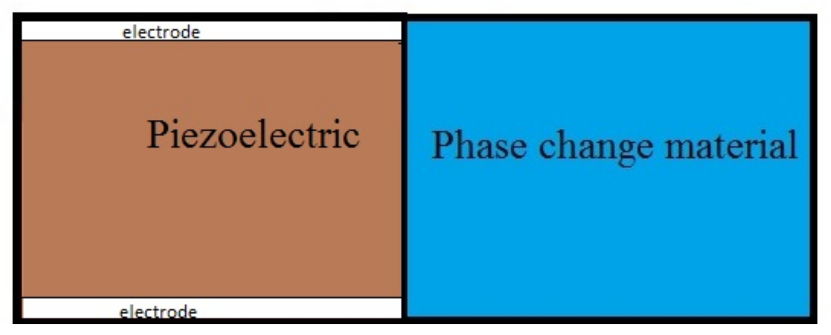
In this section governing equations and boundary conditions of the system are presented.

2.1. Cooling Part

The governing equations of fluid, the non-slip boundary conditions of fluid on walls, and the boundary condition for thermal energy are presented in

Table 1. Governing equations of fluid [2].

Equation	Conservation of
$\frac{\partial u}{\partial x}+\frac{\partial \nu }{\partial y}=0,$ (1)	mass
$\frac{\partial u}{\partial t}+u\frac{\partial u}{\partial x}+\nu \frac{\partial u}{\partial y}=$
$\frac{1}{{\rho }_{\mathrm{nf}}}(-\frac{\partial p}{\partial x}+{\mu }_{\mathrm{nf}}{\nabla }^{2}u+{\left(\rho \beta \right)}_{\mathrm{nf}}{f}_x(T-T_{\mathrm{ref}}))-\frac{{\rho }_{\mathrm{s}}}{{\rho }_{\mathrm{nf}}}\frac{\partial \varphi }{\partial x},$ (2)	x momentums
$\frac{\partial \nu }{\partial t}+u\frac{\partial \nu }{\partial x}+\nu \frac{\partial \nu }{\partial y}$
$\frac{1}{{\rho }_{\mathrm{nf}}}(-\frac{\partial p}{\partial y}+{\mu }_{\mathrm{nf}}{\nabla }^2\nu +{\left(\rho \beta \right)}_{\mathrm{nf}}{f}_y(T-T_{\mathrm{ref}}))-\frac{{\rho }_{\mathrm{s}}}{{\rho }_{\mathrm{nf}}}\frac{\partial \varphi }{\partial y},$ (3)	y momentums
$\frac{\partial T}{\partial t}+u\frac{\partial T}{\partial x}+\nu \frac{\partial T}{\partial y}$
$\frac{\partial }{\partial x}\left[\frac{(k_{\mathrm{nf}0}+k_{\mathrm{d}})}{{\left(\rho c_{\mathrm{p}}\right)}_{\mathrm{nf}}}\frac{\partial T}{\partial x}\right]+\frac{\partial }{\partial y}\left[\frac{(k_{\mathrm{nf}0}+k_{\mathrm{d}})}{{\left(\rho c_{\mathrm{p}}\right)}_{\mathrm{nf}}}\frac{\partial T}{\partial y}\right],$ (4)	energy

,

Table 2. Non-slip boundary conditions of fluid on walls [4].

x-Velocity	y-Velocity
$u(x=0,L)=0,$ (5)	$v(x=0,L)=0,$ (6)
$u(y=0,H)=0,$ (7)	$v(y=0,H)=0,$ (8)

and

Table 3. Thermal boundary conditions of fluid [8].

Wall	Equation
left	$q(x=0)=-k_{nf}\frac{\partial T(x=0)}{\partial x},$ (9)
right	$\frac{\partial T(x=L)}{\partial x}=0,$ (10)
top	$-k_{nf}\frac{\partial T(y=H)}{\partial y}=h(T(y=H)-T_{\infty }),$ (11)
bottom	$k_{nf}\frac{\partial T(y=0)}{\partial y}=h(T(y=0)-T_{\infty }),$ (12)

respectively. Enhancement of solidification rate of latent heat thermal energy storage using corrugated fins (shell-and-tube) was proved but here just a simple PCM cube is used. In some systems the PCM slurries’ density changes at phase change temperature, but here a Newtonian model is used. The nanoparticles dispersed in a phase change material can also improve melting characteristics which is neglected here.

Figure 1 shows the resonator configuration. The geometry of the BAW cell is equal to one of that circuit lines. Figure 2 illustrate the resonator and cooling part. The effective characteristics are shown in

Table 4. Nano-fluid property formulas [4].

Nano-Fluid Property	Formula
$\rho$	$(1-\alpha ){\rho }_{\mathrm{f}}+\alpha {\rho }_{\mathrm{s}},$ (13)
$\rho c_{\mathrm{p}}$	$(1-\alpha ){\left(\rho c_{\mathrm{p}}\right)}_{\mathrm{f}}+\alpha {\left(\rho c_{\mathrm{p}}\right)}_{\mathrm{s}},$ (14)
$\rho \beta$	$(1-\alpha ){\left(\rho \beta \right)}_{\mathrm{f}}+\alpha {\left(\rho \beta \right)}_{\mathrm{s}},$ (15)
$\mu$	$\frac{{\mu }_{\mathrm{f}}}{{(1-\alpha )}^{2.5}},$ (16)
k	$k_{\mathrm{f}}\frac{k_{\mathrm{s}}+2k_{\mathrm{f}}-2\alpha (k_{\mathrm{f}}-k_{\mathrm{s}})}{k_{\mathrm{s}}+2k_{\mathrm{f}}+\alpha (k_{\mathrm{f}}-k_{\mathrm{s}})}+C{\left(\rho c_{\mathrm{p}}\right)}_{\mathrm{nf}}\sqrt{u^2+{\nu }^2}\alpha d_{\mathrm{p}},$ (17)
$\rho L$	$(1-\alpha ){\left(\rho L\right)}_{\mathrm{f}},$ (18)
$\sigma$	${\sigma }_f\left(1+\frac{3\left({\sigma }_{\mathit{s}}-{\sigma }_f\right)\varphi }{\left({\sigma }_{\mathit{s}}+2{\sigma }_f\right)-\left({\sigma }_{\mathit{np}}-{\sigma }_f\right)\varphi }\right),$ (19)

while the material thermophysical properties are presented in

Table 5. Material thermo-physical properties [2].

Material	k (W/m·K)	C (kJ/kg·K)	$\mathit{\rho }$ (kg/m${}^3$)	$\mathit{\beta }$(K${}^{-1}$)	${\mathit{H}}_{\mathit{f}}$ (J/kg )	$\mathit{\mu }$(Pa·s)
fluid TH29	0.53	2.2	1530	$2\times {10}^{-4}$	187	$5.33\times {10}^{-3}$
solid TH29	1.09	1.4	1719		187
Cu	400	0.383	8954	$1.67\times {10}^{-5}$

. The effect of the addition of nanoparticle on the thermal behavior of PCM is obtainable from Table 4. Many fluids and solids such as organic materials, carb-oxy-methyl cellulose carbon foams, paraffin, and expanded graphite are used as phase change material previously for a thermal storage system. However, here TH29 was selected as [2,29].

Graphs of heat flow (in joule per second) as a function of temperature which is called in literature the differential scanning calorimeter (DSC), usually provided by PCM producers. TH29 (Calcium-chloride hexahydrate) performance in DSC form is presented in [29] for the pure material and its mixing with cellulose. As well, the TH29 shows good performance in aged cases which exposes to ambient air for two weeks. From the mass measurements, the hydrated salt-based TH29 absorbed moisture at about $50\%$ of their weight and lost their ability in eight days.

As well, various nanoparticles were used such as Ag, carbon nanofiber, Al, aluminum, and carbon nanotubes. However, here copper nanoparticle was used. The governing equations and thermal boundary conditions for heat transfer in solid part are presented in

Table 6. Governing equations and thermal boundary conditions for heat transfer in solid part [6].

Zone	Equation
thermal balance over volume	$\frac{\partial T}{\partial t}=\frac{\partial }{\partial x}\left[\frac{k_{\mathrm{s}}}{{\rho }_s{c}_{\mathrm{s}}}\frac{\partial T}{\partial x}\right]+\frac{\partial }{\partial y}\left[\frac{k_{\mathrm{s}}}{{\rho }_s{c}_{\mathrm{s}}}\frac{\partial T}{\partial y}\right]+\frac{\dot{q}\prime \prime \prime }{{\rho }_s{c}_s},$ (20)
left wall	$\frac{\partial T(x=-B)}{\partial x}=0,$ (21)
right wall	$q(x=0)=-k_s\frac{\partial T(x=0)}{\partial x},$ (22)
top wall	$-k\frac{\partial T(y=H)}{\partial y}=h(T(y=H)-T_{\infty }),$ (23)
bottom wall	$k\frac{\partial T(y=0)}{\partial y}=h(T(y=0)-T_{\infty }),$ (24)

.

Usually, the thermal delay method is used to determine the effective characteristics of micro-encapsulated phase change material. Table 5 mentions TH29, a commercially available PCM.

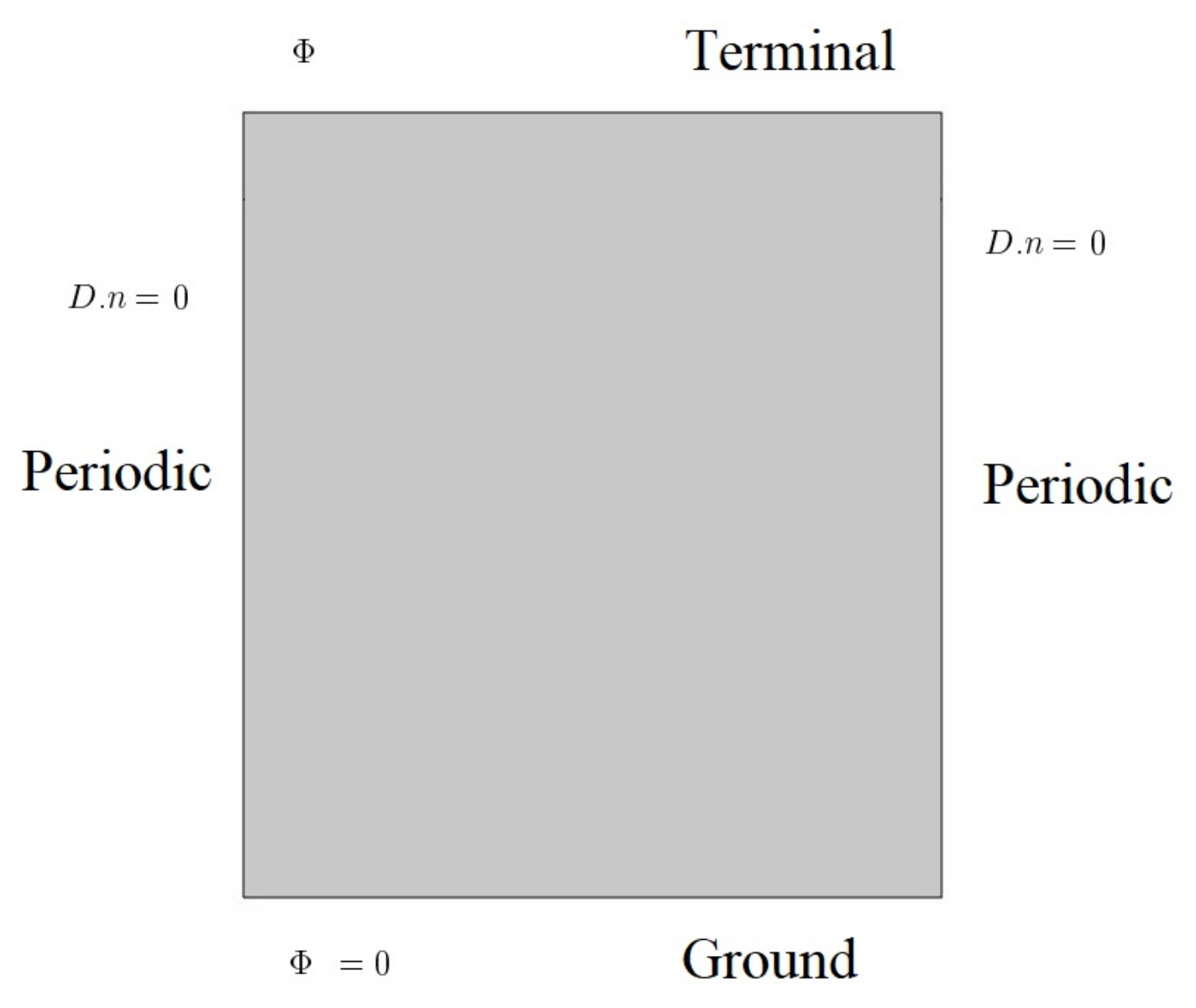
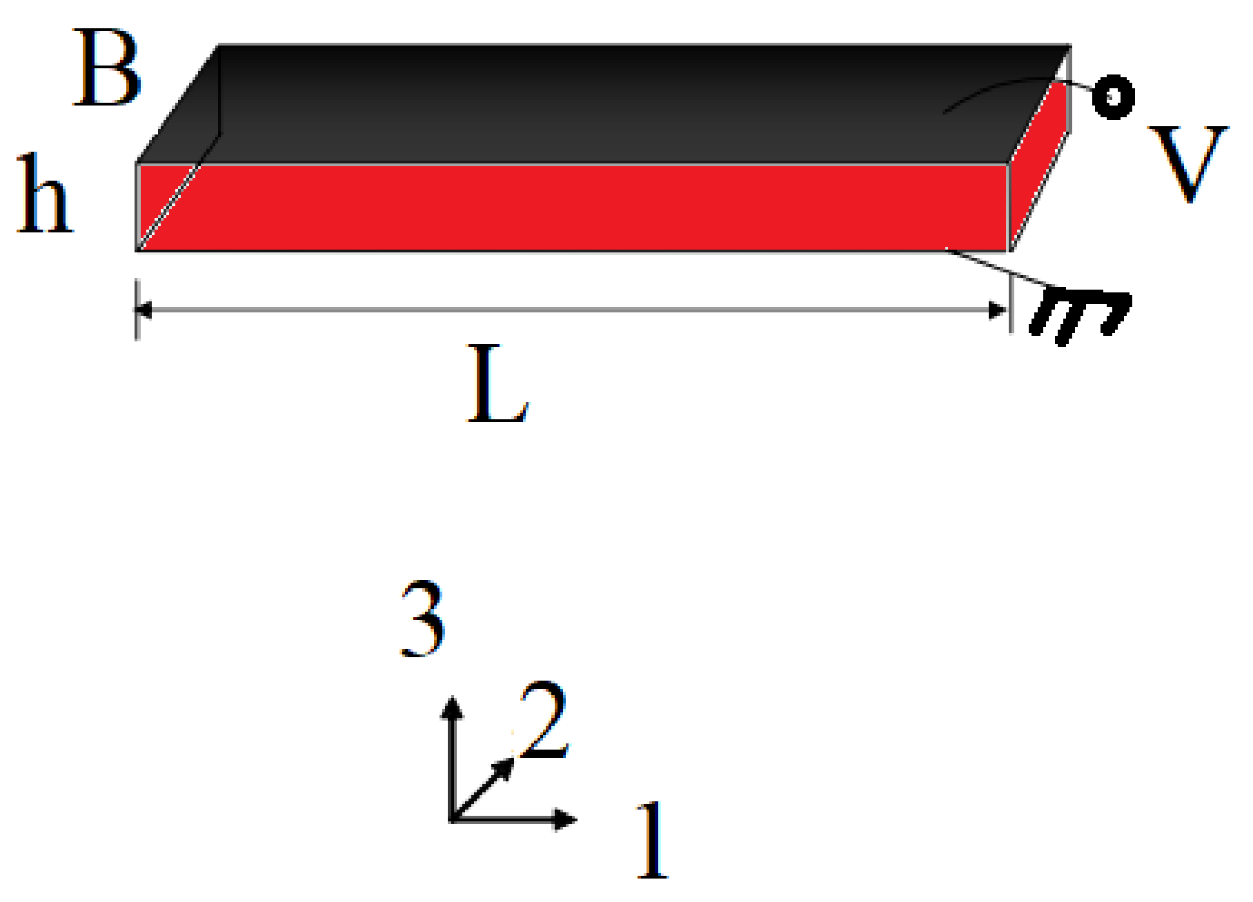
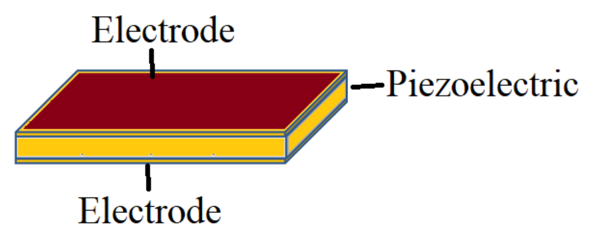
2.2. Piezoelectric Induced Wave

The piezoelectric constitutive conditions that couple the mechanical and electrical amounts in the piezoelectric material are communicated utilizing the coupling equations. The conservation of momentum for the bulk acoustic wave in an electrical part is presented in

Table 7. Conservation of momentum for bulk acoustic wave in electrical part [6].

Zone	Equation
momentum conservation	$\rho \frac{{\partial }^2}{\partial t^2}\left[\begin{array}{ccc}u& v& w\end{array}\right]=\left[\begin{array}{ccc}\frac{\partial }{\partial x}& \frac{\partial }{\partial y}& \frac{\partial }{\partial z}\end{array}\right]\left[\begin{array}{ccc}{T}_{11}& T_{12}& T_{13}\\ T_{12}& T_{22}& T_{23}\\ T_{13}& T_{23}& T_{33}\end{array}\right],$ (25)
periodic left and right walls	${\mathbf{u}}_{destination}={\mathbf{u}}_{source}{e}^{(-i\mathbf{k}}({\mathbf{r}}_{destination}-{\mathbf{r}}_{source\left)\right)},$ (26)
top and bottom free surfaces	$\mathbf{T}.\mathbf{n}=0,$ (27)

.

The electrical boundary condition for the piezoelectric wave is depicted in Figure 3. The wave motion ($\rho \frac{{\partial }^2{u}_i}{\partial t^2}=\frac{\partial T_{ij}}{\partial x_j}$) which comes from conservation of momentum and presented in in Table 7. The coupled constitutive equations in strain-charge form [6] are

$$\begin{array}{c}\hfill \left[\begin{array}{c}{S}_{11}\\ S_{12}\\ S_{13}\\ S_{22}\\ S_{23}\\ S_{33}\end{array}\right]=\\ \hfill \left[\begin{array}{cccccc}{\mathit{s}}_{11}^E& {\mathit{s}}_{12}^E& {\mathit{s}}_{13}^E& 0& 0& 0\\ {\mathit{s}}_{12}^E& {\mathit{s}}_{22}^E& {\mathit{s}}_{23}^E& 0& 0& 0\\ {\mathit{s}}_{13}^E& {\mathit{s}}_{23}^E& {\mathit{s}}_{33}^E& 0& 0& 0\\ 0& 0& 0& {\mathit{s}}_{44}^E& 0& 0\\ 0& 0& 0& 0& {\mathit{s}}_{55}^E& 0\\ 0& 0& 0& 0& 0& {\mathit{s}}_{66}^E\end{array}\right]\left[\begin{array}{c}{T}_{11}\\ T_{12}\\ T_{13}\\ T_{22}\\ T_{23}\\ T_{33}\end{array}\right]-& \\ \hfill \left[\begin{array}{ccc}0& 0& {\mathit{d}}_{31}\\ 0& 0& {\mathit{d}}_{32}\\ 0& 0& {\mathit{d}}_{33}\\ 0& {\mathit{d}}_{24}& 0\\ {\mathit{d}}_{15}& 0& 0\\ 0& 0& 0\end{array}\right]\left[\begin{array}{c}\frac{\partial \varphi }{\partial x}\\ \frac{\partial \varphi }{\partial y}\\ \frac{\partial \varphi }{\partial z}\end{array}\right]\end{array}$$

(28)

and

$$\begin{array}{cc}\hfill \left[\begin{array}{c}{D}_1\\ D_2\\ D_3\end{array}\right]=\left[\begin{array}{cccccc}0& 0& 0& 0& {\mathit{d}}_{15}& 0\\ 0& 0& 0& {\mathit{d}}_{25}& 0& 0\\ {\mathit{d}}_{31}& {\mathit{d}}_{32}& {\mathit{d}}_{33}& 0& 0& 0\end{array}\right]\left[\begin{array}{c}{T}_{11}\\ T_{12}\\ T_{13}\\ T_{22}\\ T_{23}\\ T_{33}\end{array}\right]-& \\ \hfill \left[\begin{array}{ccc}{\epsilon }_{11}^T& 0& 0\\ 0& {\epsilon }_{22}^T& 0\\ 0& 0& {\epsilon }_{33}^T\end{array}\right]\left[\begin{array}{c}\frac{\partial \varphi }{\partial x}\\ \frac{\partial \varphi }{\partial y}\\ \frac{\partial \varphi }{\partial z}\end{array}\right]\end{array}$$

(29)

Consider next the case where the slab is electrically excited by applying a harmonic voltage, v = $V_0{e}^{jt}$, across the electrodes. In this case, it is convenient to consider a slab of length L with ends at x = L/2. The stresses at the ends are zero. The fields of interest are expressed by eigenfrequency analysis ($-\rho {\omega }^{2}u=\frac{\partial T_{11}}{\partial x}$). The dielectric permittivity, elastic and piezoelectric constants of ZnO are considered in this study.

As the velocity of the electromagnetic wave is faster than the acoustic wave, the electrostatic equation of Laplace is applied for electric potential (${\nabla }^2\varphi =0$). As well, the electrical displacement is the function of strain and the electric field ($D_i=d_{ikl}{S}_{kl}+{\epsilon }_{ik}^T{E}_k$).

3. Results

Here, predominantly, the instance of voltage stacking is considered, i.e., one terminal is electrically grounded, and a sinusoidal voltage with endorsed consistent plentifulness is associated between the grounded and “hot” anode. Arrangement of the eigenvalue issue at that point brings about arrangement reverberation frequencies (short-circuited terminals) at which the electrical impedance expects low qualities. The equal reverberation frequencies with enormous estimations of impedance can be acquired from the open-circuited case. For the open-circuit limit conditions, the potential is set consistent on the “hot” anode, yet not fixed (drifting potential).

In this section which describes the results, first, the confrontation of the obtained results with other research are presented through validations. Such a suitable comparison significantly raises the meaning of the presented paper. Then the effect of adding PCM to BAW is discussed.

3.1. Validation of Used Code

In this section, various parts of the code are validated against well-known benchmarks and commercial software.

3.1.1. Validation of Fluid Part

For the purpose of the validation of the fluid part, the previous work of Jamalabadi and Park [2] is used. The vertical axis in Figure 4 is solid content that has no unit. As revealed in Figure 4 the solid percent of PCM decreased by the increase of time (melting process). As seen in Figure 4 both methods are in good agreement.

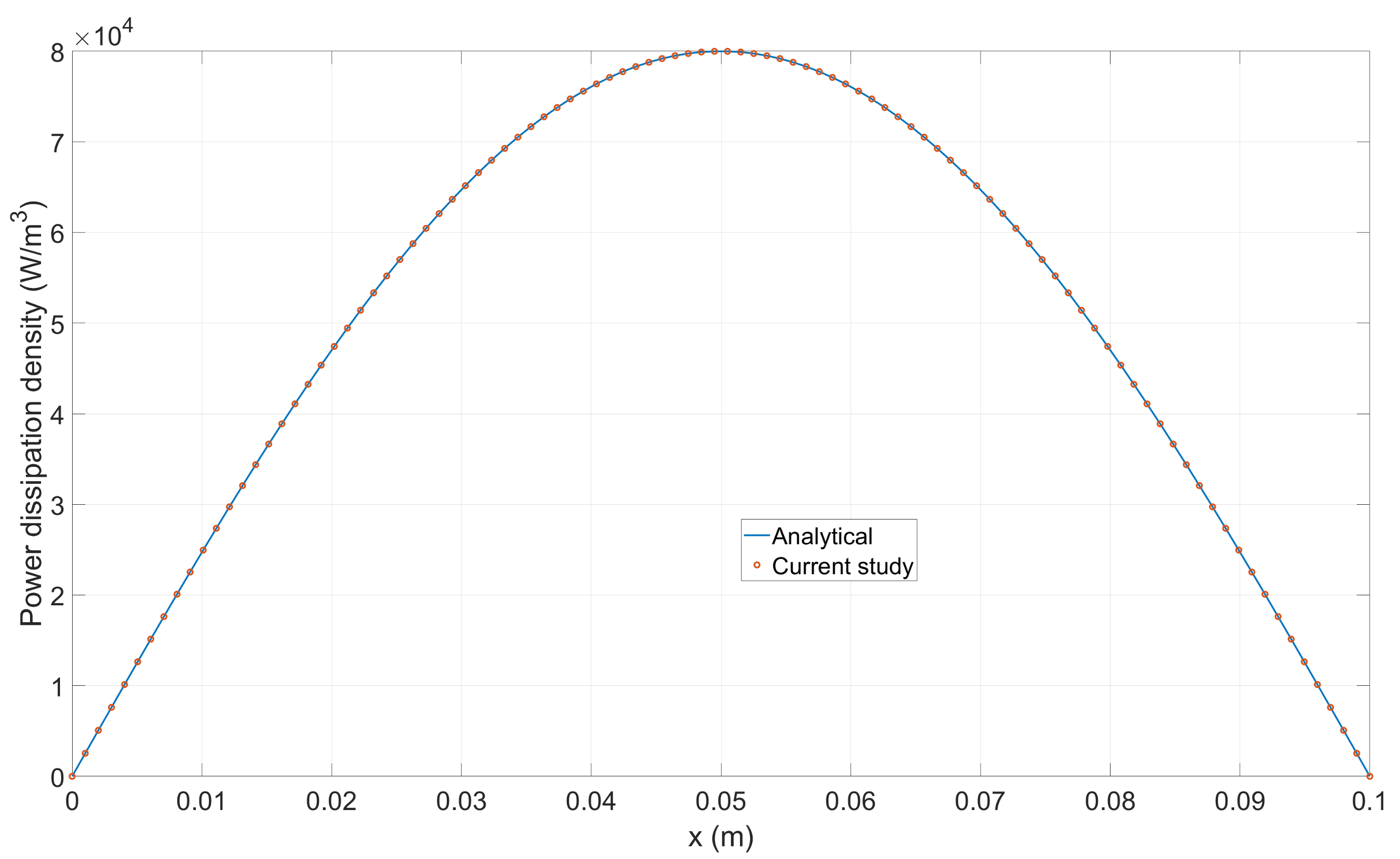
3.1.2. Validation of Heat Generation

In this section, the validation of heat generation caused by resonance with the analytical solution is performed. The loss mechanisms in the thin film BAW resonators include leakage to the substrate, laterally escaping waves, ohmic losses, viscous losses, dielectric losses, and wave scattering. Additionally mentioned in the literature are eddy current losses and losses due to the formation of conducting channels in the high resistivity substrate interface. The analytical solution of the piezoelectric governing equation for heat generation is given in Appendix A. To calculate the heat generation of the electric source, both mechanical part (elastic energy) and electric part (electric displacement energy) should be considered. The Poynting vector (W/m${}^2$) which is the directional energy flux (the energy transfer per unit area per unit time) usually used as a symbol of conservation of electromagnetic energy ($S=E\times H$). The basic idea is that Poynting energy losses some parts as passed through the piezoelectric material and electrodes. Here the power loss distribution when the slab is electrically excited by an applied voltage is considered. The electrical excitation with the amplitude of 10 V is applied across the terminals. Material and geometrical parameters for the case of heat generation are presented in Figure 5 and

Table 8. Material and geometrical parameters for the case of heat generation.

Parameter	Value	Unit
L	100	mm
B	10	mm
h	5	mm
$\rho$	7500	kg/m${}^3$
$d_{31}$	$-123\times {10}^{-12}(1-j\times 0.005)$	C/N
${ϵ}_{33}^T$	$1300\times 8.854\times {10}^{-12}(1-j\times 0.004)$	F/m
$s_{11}^E$	$12.3\times {10}^{-12}(1-j\times 0.005)$	F/m

.

The comparison of the current code with the analytical solution which is given in Appendix B is plotted in Figure 6. As seen in Figure 6 both numerical and analytical results are in good agreement. The validation results of Figure 6 has the error of simulation near zero as it designed to respond in 1D and the effect of transverse direction is not too much as the electrode extends all over the top and bottom surface. In engineering applications, the electrodes cover the surface partially and some materials are added to help the system to have these ideal mechanical support connections.

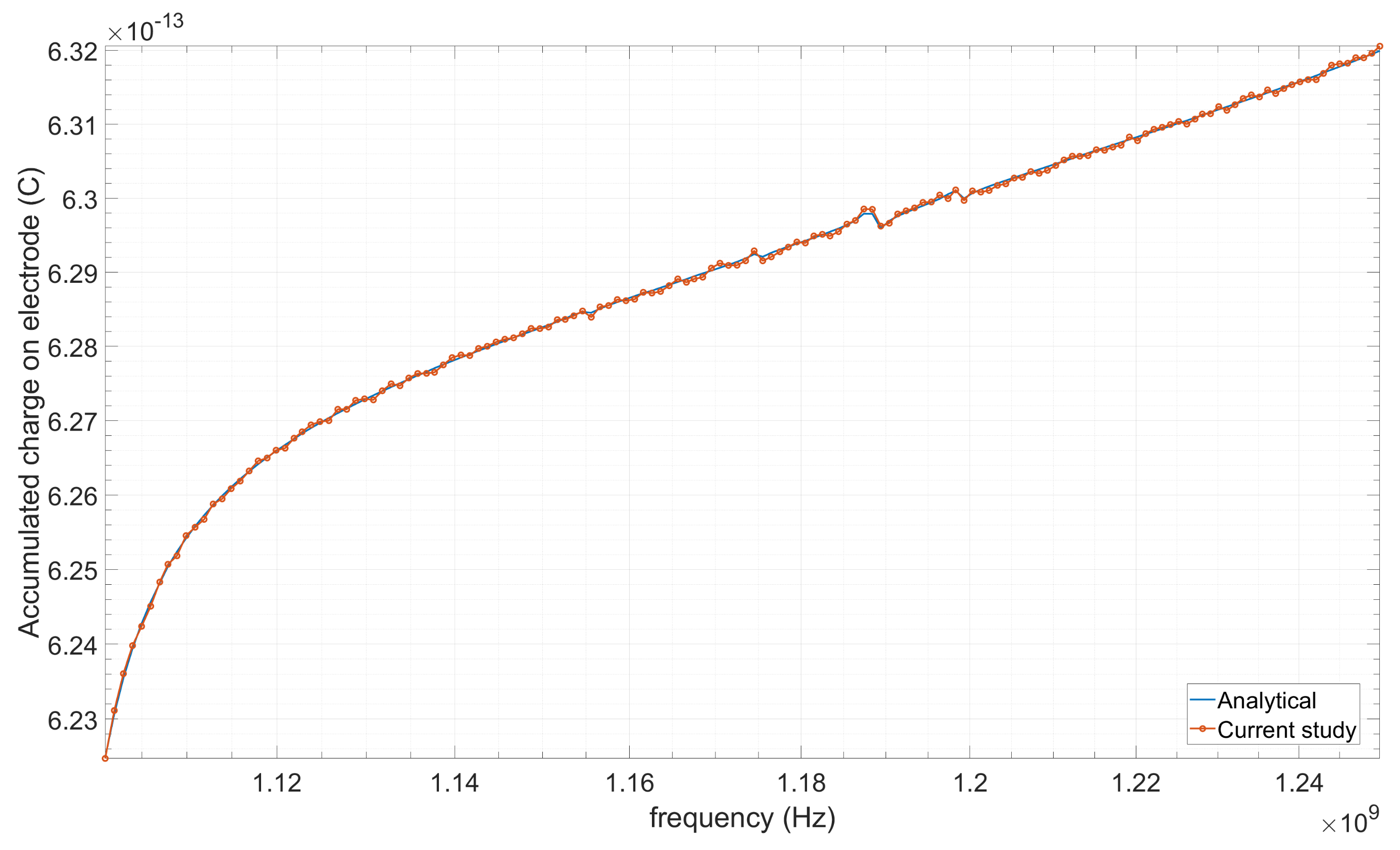
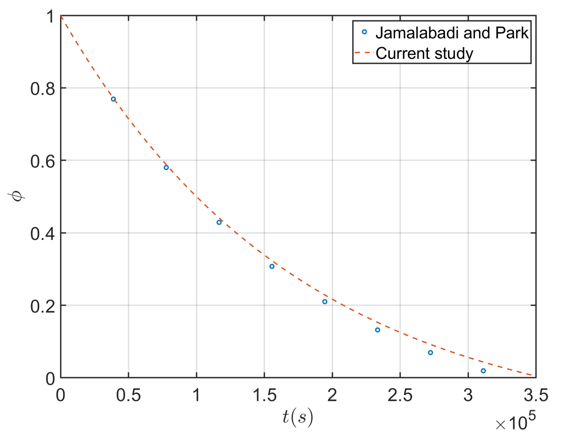
3.1.3. Validation of Charge Curve

In this section, the 3D problem is considered while in another part of the paper you can consider the 2D model as the third direction has not affected the results. Simulation of a conventional BAW resonator is performed in the appendix code presented at the end of the paper. After a variable definition on substrate, electro, piezo, and resonator parameters. Element types of solid226 and solid95 are used to model the piezoelectric parts. Materials parameters of aluminum nitride for various directions as anisotropic material in the form of tabular data are given. Some damping parameters are also considered for mechanical and electrical losses. Silicon and molybdenum data are entered as well. For building geometry, the bottom substrate, bottom electrode, piezo layers, and top electrode simple block are used. 3D regular mesh is created to apply the mechanical boundary conditions (two symmetry faces, right surface from top view symmetry, and up to surface from top view symmetry, down surface from top view hard boundary as a fixed plate) and electrical boundary conditions (electrode bottom, electrode top). The results of harmonic analysis in a range of 1100 and 1250 Mhz are used to validate the charge collected on the electrode surface. Material parameters definition and geometry of the compared case are presented in

Table 9. Material parameters definition.

Material Name	Parameter	Value
Aluminum Nitride	$\rho$	3260
	${\nu }_x$	8
	${\nu }_y$	8
	${\nu }_z$	10
Silicon	$\rho$	2181.5
	E	$176.52\times {10}^9$
	$\nu$	0.22
	G	$72.345\times {10}^9$
Molybdenum	$\rho$	10096
	E	$232.36\times {10}^9$
	$\nu$	0.362
	G	$85.3\times {10}^9$

and

Table 10. Variable definition.

Variable Name	Value
$x_{subs}$	$200\times {10}^{-6}$
$y_{subs}$	$200\times {10}^{-6}$
$z_{subs}$	$5\times {10}^{-7}$
$x_{electro,bot}$	$200\times {10}^{-6}$
$y_{electro,bot}$	$200\times {10}^{-6}$
$z_{electro,bot}$	$200\times {10}^{-9}$
$x_{electro,top}$	$150\times {10}^{-6}$
$y_{electro,top}$	$150\times {10}^{-6}$
$z_{electro,top}$	$260\times {10}^{-9}$
$x_{piezo}$	$200\times {10}^{-6}$
$y_{piezo}$	$200\times {10}^{-6}$
$z_{piezo}$	$1\times {10}^{-6}$

, respectively. As seen the piezoelectricity and full anisotropy of the materials are taken into account. The comparison of the current code with the ANSYS-APDL code results which the code is provided in Appendix B is plotted in Figure 7. As seen in the figure, both results are in good agreement. The validation results of Figure 7 have the error of simulation near zero. As both used the same method (FEM) these results were anticipated.

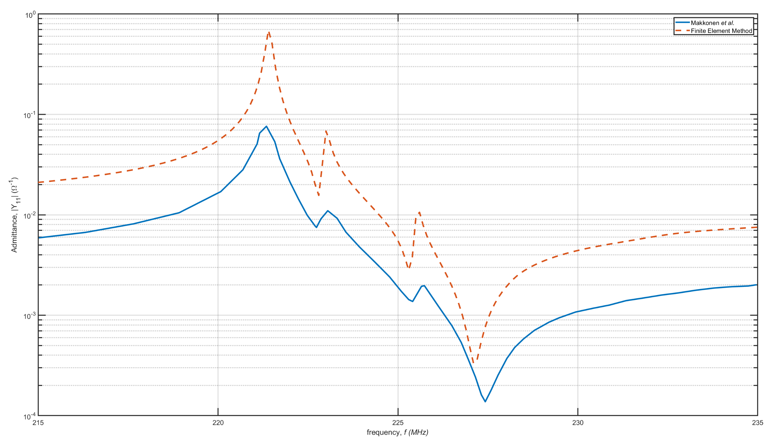
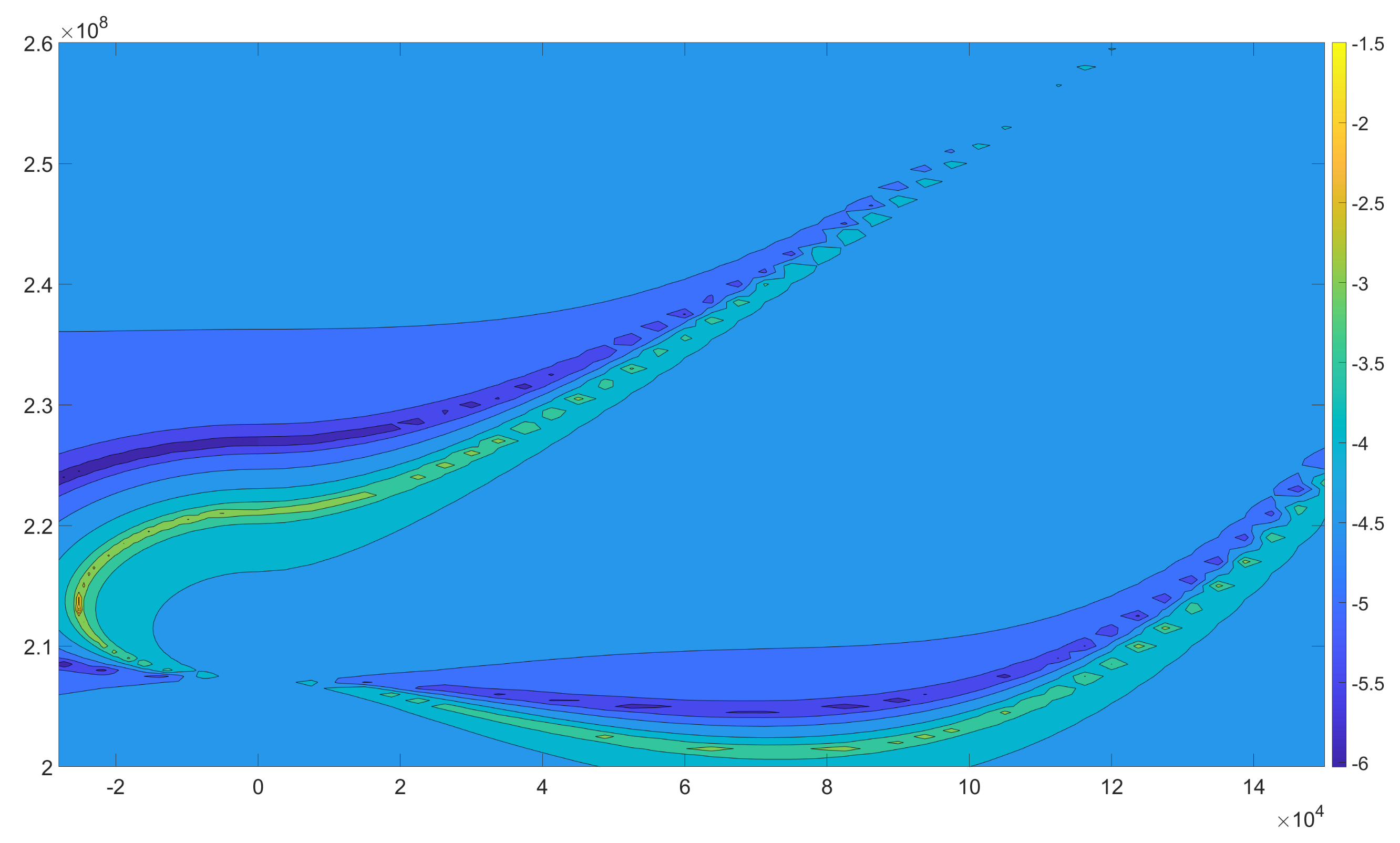
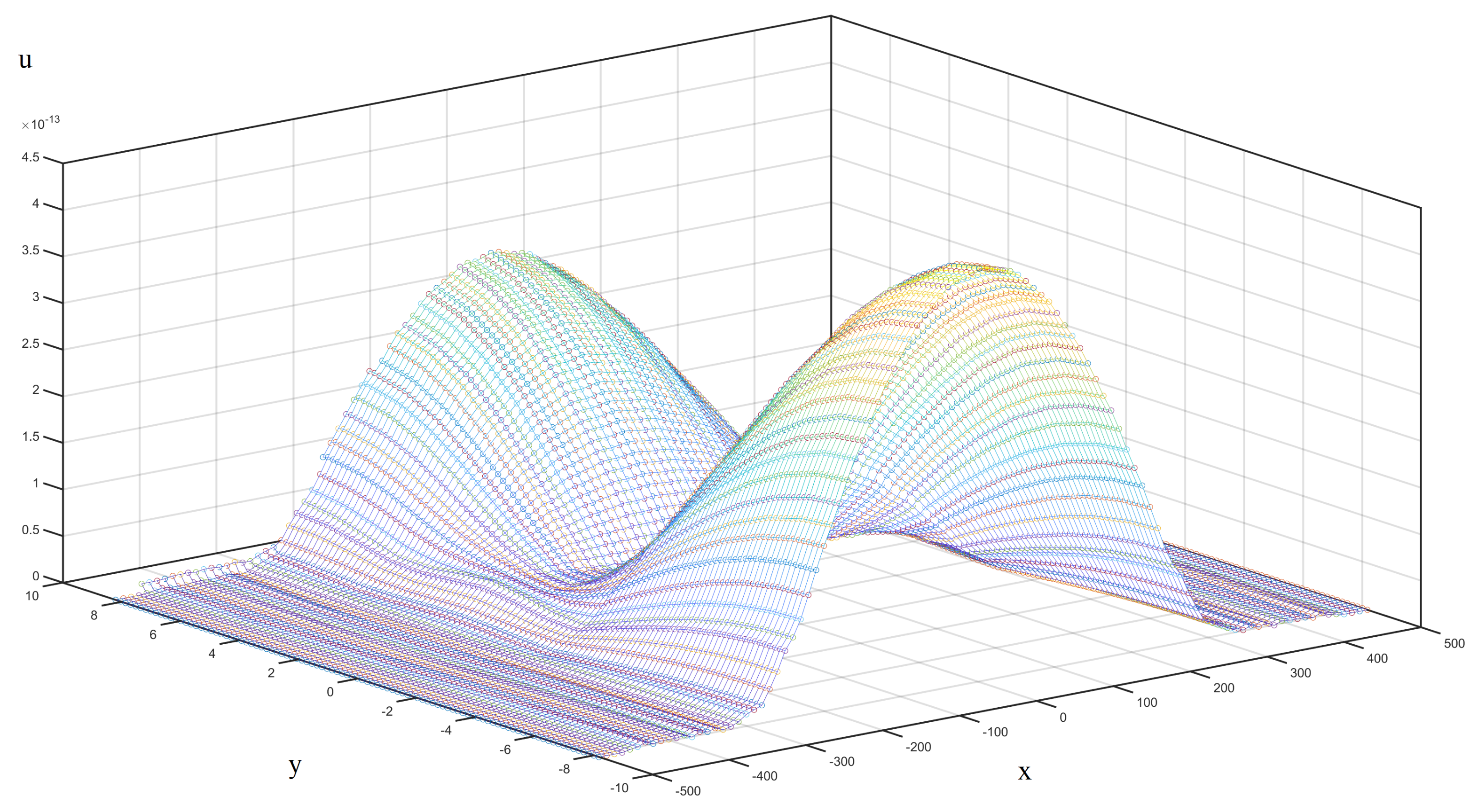
3.1.4. Validation of Dispersion Curve

The behavior of the side resonances in a multilayer structure is a function of Lamb modes curves traveling in a multilayer structure is investigated in this section. The comparison of a dispersion curves presented by Makkonen et al. [3] is given in Figure 8. As depicted in the Figure 8, both methods are in good agreement.

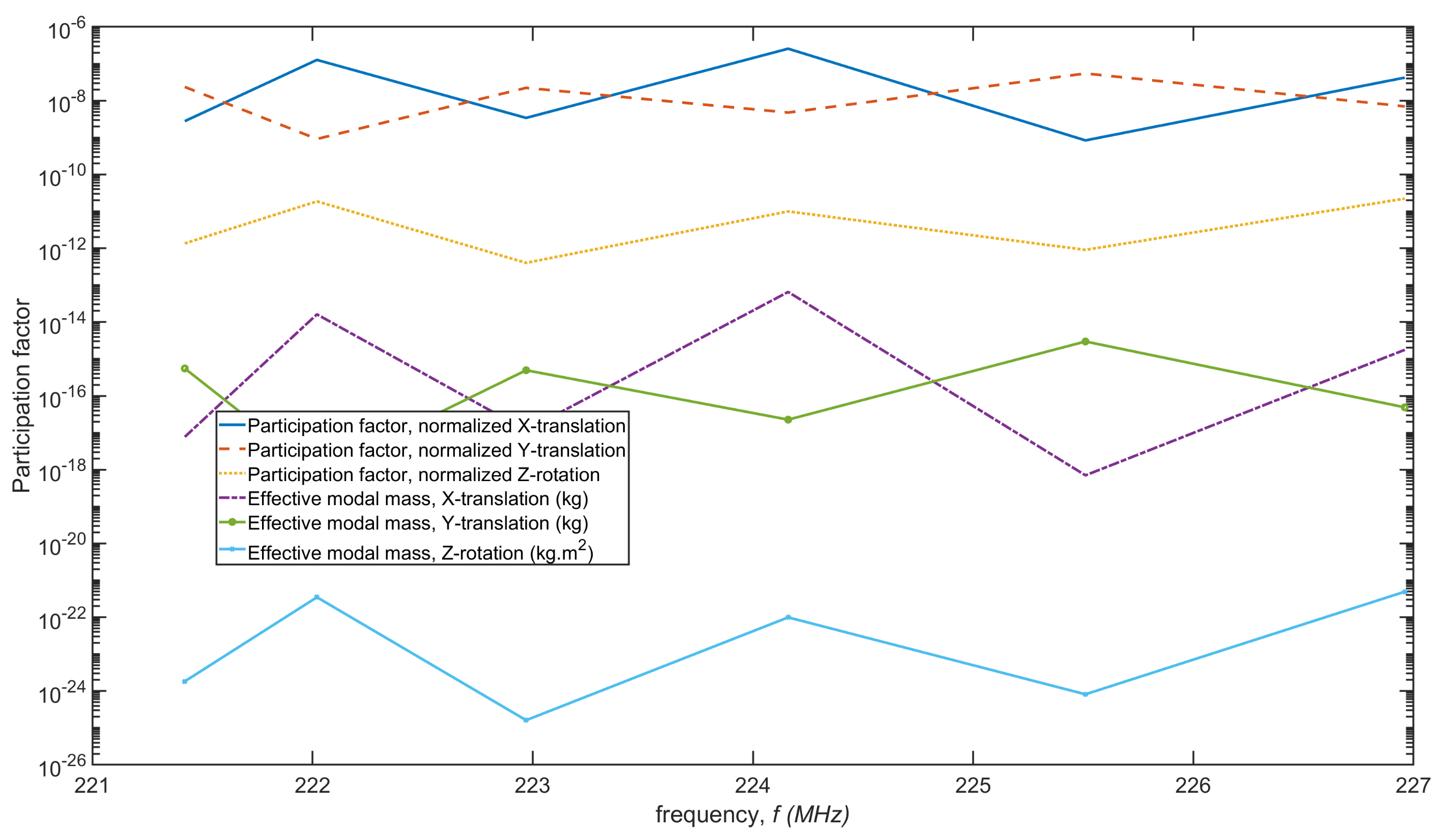
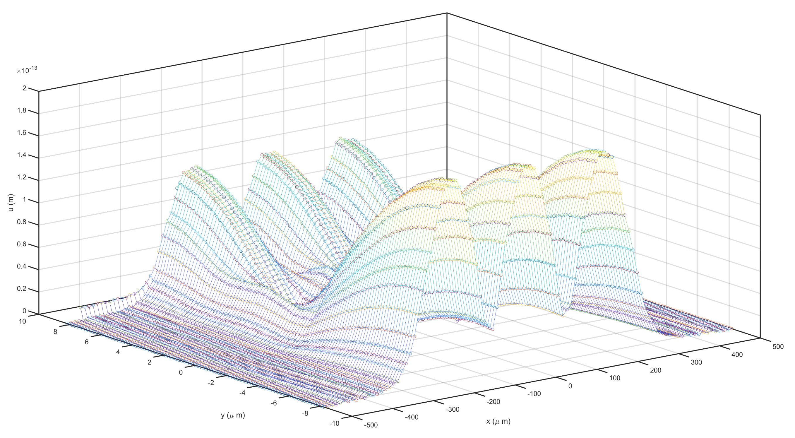
3.2. Eigenfrequency Analysis

The first six modes of the BAW problem are presented in this part. The real part of the first six modes of BAW device is 221.4200 222.02, 222.97, 224.16, 225.51, and 226.96 MHz. The imaginary parts are three orders of magnitude less than the real parts with the values of 83.593, 84.982, 84.029, 90.701, 90.162, and 90.142 kHz. Detailed parameters are given in

Table 11. Eigenfrequency study of six modes of BAW resonator.

Description	Units	Value
Eigenfrequency	Hz	221.42 + 0.083574i
Participation factor, normalized, X-translation	-	−1.4177E−9−2.3951E−9i
Participation factor, normalized, Y-translation	-	2.3391E−8−2.3982E−9i
Participation factor, normalized, Z-rotation	−	1.3453E−12 + 1.4519E−13i
X-translation modal mass	kg	−3.7265E−18 + 6.7912E−18i
Y-translation modal mass	kg	5.4141E−16−1.1219E−16i
Z-rotation modal mass	kg·m${}^2$	1.7886E−24 + 3.9064E−25i
Eigenfrequency	Hz	222.02 + 0.084982i
Participation factor, normalized, X-translation	-	−1.2376E−7−2.2132E−8i
Participation factor, normalized, Y-translation	-	−6.3621E−10 + 1.2395E−9i
Participation factor, normalized, Z-rotation	−	−7.0904E−12 + 1.7065E−11i
X-translation modal mass	kg	1.4827E−14 + 5.4782E−15i
Y-translation modal mass	kg	−1.1316E−18−1.5772E−18i
Z-rotation modal mass	kg·m${}^2$	−2.4093E−22−2.4199E−22i
Eigenfrequency	Hz	222.97 + 0.084029i
Participation factor, normalized, X-translation	-	2.3988E−9−8.4602E−10i
Participation factor, normalized, Y-translation	-	−1.0829E−8−2.0163E−8i
Participation factor, normalized, Z-rotation	−	−1.1635E−13−1.7268E−13i
X-translation modal mass	kg	5.0385E−18−4.0589E−18i
Y-translation modal mass	kg	−2.8925E−16 + 4.3670E−16i
Z-rotation modal mass	kg·m${}^2$	−1.6281E−26 + 4.0181E−26i
Eigenfrequency	Hz	224.16 + 0.090701i
Participation factor, normalized, X-translation	-	5.3732E−8−2.4727E−7i
Participation factor, normalized, Y-translation	-	6.2749E−10−1.0431E−9i
Participation factor, normalized, Z-rotation	−	−6.0091E−12−6.5558E−12i
X-translation modal mass	kg	−5.8254E−14−2.6572E−14i
Y-translation modal mass	kg	−6.9441E−19−1.3091E−18i
Z-rotation modal mass	kg·m${}^2$	−6.8693E−24 + 7.8788E−23i
Eigenfrequency	Hz	225.51 + 0.090162i
Participation factor, normalized, X-translation	-	−2.9494E−9−1.3085E−9i
Participation factor, normalized, Y-translation	-	−3.4432E−9 + 5.0666E−8i
Participation factor, normalized, Z-rotation	−	6.7515E−13 + 6.2670E−13i
X-translation modal mass	kg	6.9867E−18 + 7.7184E−18i
Y-translation modal mass	kg	−2.5551E−15−3.4891E−16i
Z-rotation modal mass	kg·m${}^2$	6.3072E−26 + 8.4624E−25i
Eigenfrequency	Hz	226.96 + 0.090142i
Participation factor, normalized, X-translation	-	3.8473E−8−1.7100E−8i
Participation factor, normalized, Y-translation	-	−1.0000E−9−9.8674E−10i
Participation factor, normalized, Z-rotation	−	−2.1903E−11 + 6.6730E−12i
X-translation modal mass	kg	1.1878E−15−1.3158E−15i
Y-translation (modal mass	kg	2.6426E−20 + 1.9736E−18i
Z-rotation modal mass	kg·m${}^2$	4.3522E−22−2.9232E−22i

. To have a better understanding of given parameters they have been plotted in Figure 9. As shown, the coefficients have a fluctuation from one frequency to another. In participation factors of x and z, even frequencies ($2,4,6,\dots$) have higher values and y participation factors have maximum in odd frequencies ($1,3,5,\dots$).

Figure 10, Figure 11, Figure 12, Figure 13, Figure 14 and Figure 15 show horizontal and vertical displacement of mode 1 to mode 3. Each of propagating modes and evanescent modes can also be visualized by its displacement field. As seen in Figure 10, the horizontal displacement of mode 1 has two peaks at the middle of terminals. Figure 11 presents four peaks in the vertical displacement of mode 1 where one of them is in opposite direction. Horizontal displacement of mode 2 as expected has four ($2\times N$) peaks which are symmetric around the middle of piezoelectric which is visible in Figure 12. As illustrated in Figure 13, vertical displacement of mode 2 has four maximum and four minimum which are aligned in three parallel lines. The presence of propagating and evanescent modes is clear. The exhibition of six ($2\times N$) simple maximum of mode 3 of horizontal displacement of mode 3 is demonstrated in Figure 14. As shown the eigenfunctions are aligned in three parallel lines and are symmetric conditions. Finally, the eigenfunctions of mode 3 of vertical displacement with six visible maximum are depicted in Figure 15. A detailed BAW design, general discussion on BAW resonators, and electric potential modes are discussed in [1,6]. In surface plotted figures including Figure 10, Figure 11, Figure 12, Figure 13, Figure 14 and Figure 15 the color is automatically proportional to surface height.

The damping ration, quality factor, and $S_{11}$ are plotted in Figure 16, Figure 17 and Figure 18 respectively. Damping ratio (ratio of imaginary of the frequency to its absolute value) and quality factor (ratio of absolute value to two times of the imaginary of the frequency) as a function of frequency are plotted in Figure 16. The quality factor for frequency as a function of frequency is depicted in Figure 17. The real part and the imaginary part of the scattering parameter as a function of frequency are illustrated in Figure 18 for the layer structure of a BAW resonator. Here the quality plot is against all selected intervals of frequency. The dispersion curve of imaginary (evanescent mode) and real (propagating mode) parts of the wavenumbers are figured in Figure 19 for a thin-film BAW composite resonator. The dispersion schematic includes both imaginary and real parts of the wavenumber. The plots actually are the contours of admittance $|Y_{11}|$ for real part of k, and contours of admittance $|Y_{22}|$ for imaginary the part of k. Figure 19 shows the calculated dispersion curve. The results for the the real and the imaginary parts of the wavenumber are combined by taking the positive k-axis with an optimum near $(6\times {10}^4,2\times {10}^8)$ for the real part and the negative k-axis with a maximum near $(-2\times {10}^4,2\times {10}^8)$ for the imaginary part. The horizontal axis of dispersion curve is k, wave number, with the unit of $\frac{1}{m}$ while the vertical axis is f, frequency, with aunit of $\frac{1}{s}$. They correspond to the lower branch for the $T{S}_2$ mode (thickness-shear), the upper branch for the $T{E}_1$ mode (thickness-extension), and the left branch for the evanescent modes.

Total power dissipation as a function of frequency is plotted in Figure 20 for the specific device structure thin-film BAW composite resonator considered here. As shown, the maximum value of heat generation happened in the first mode while is in accordance with maximum admittance ($Y_{11}$). This graph will be used in the next part as the input for heat generation.

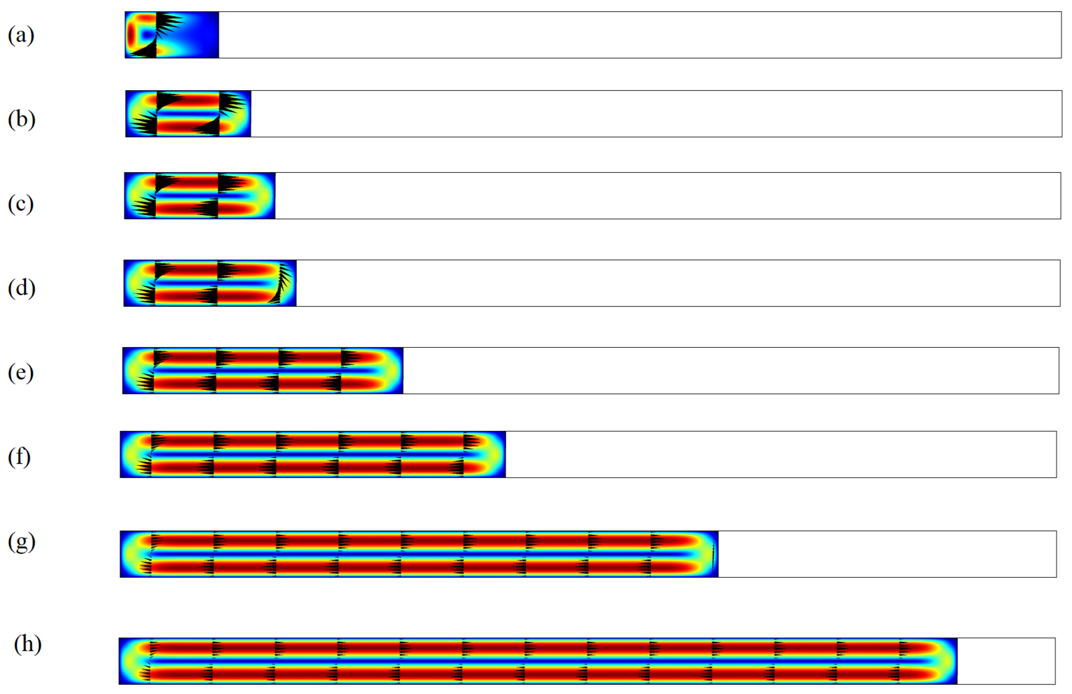
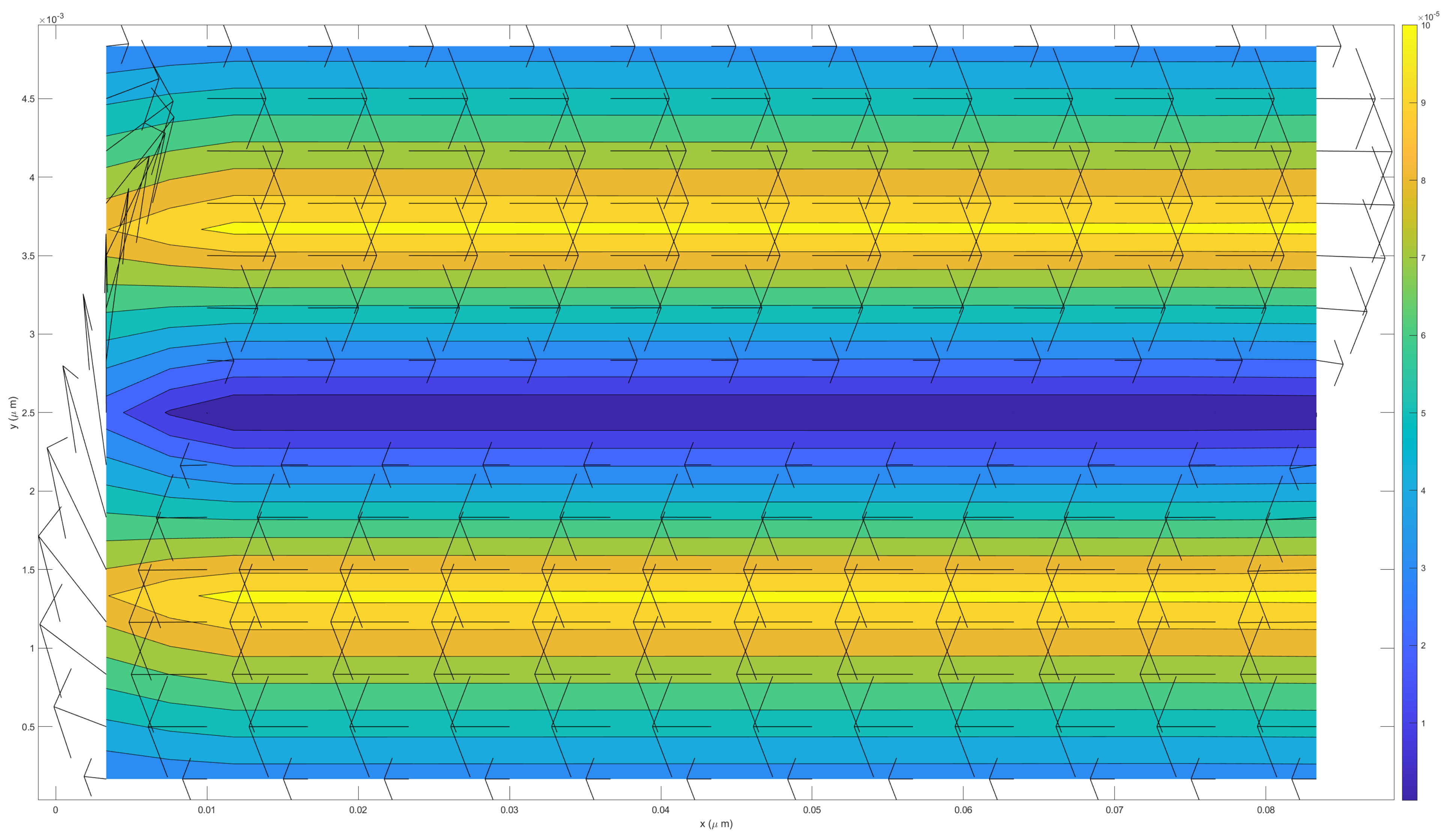
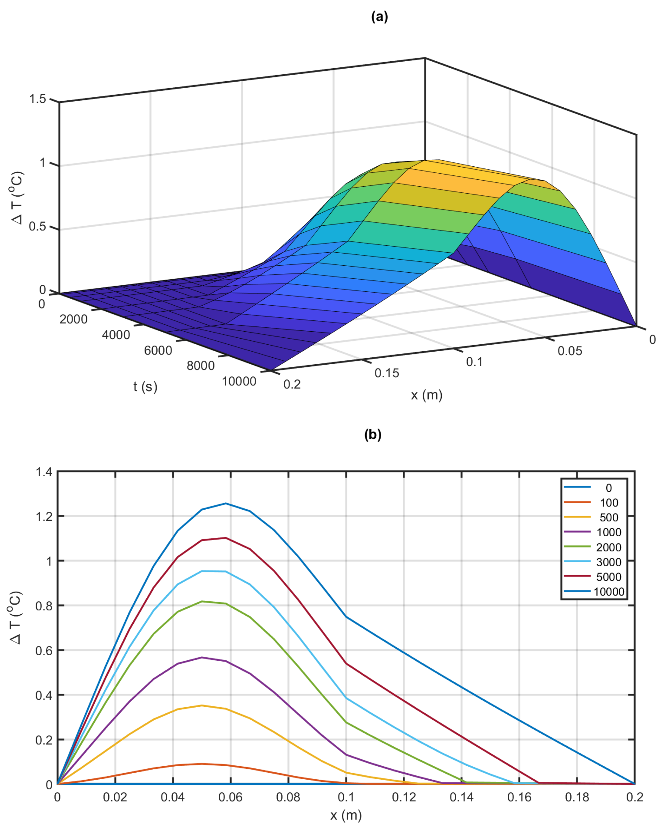
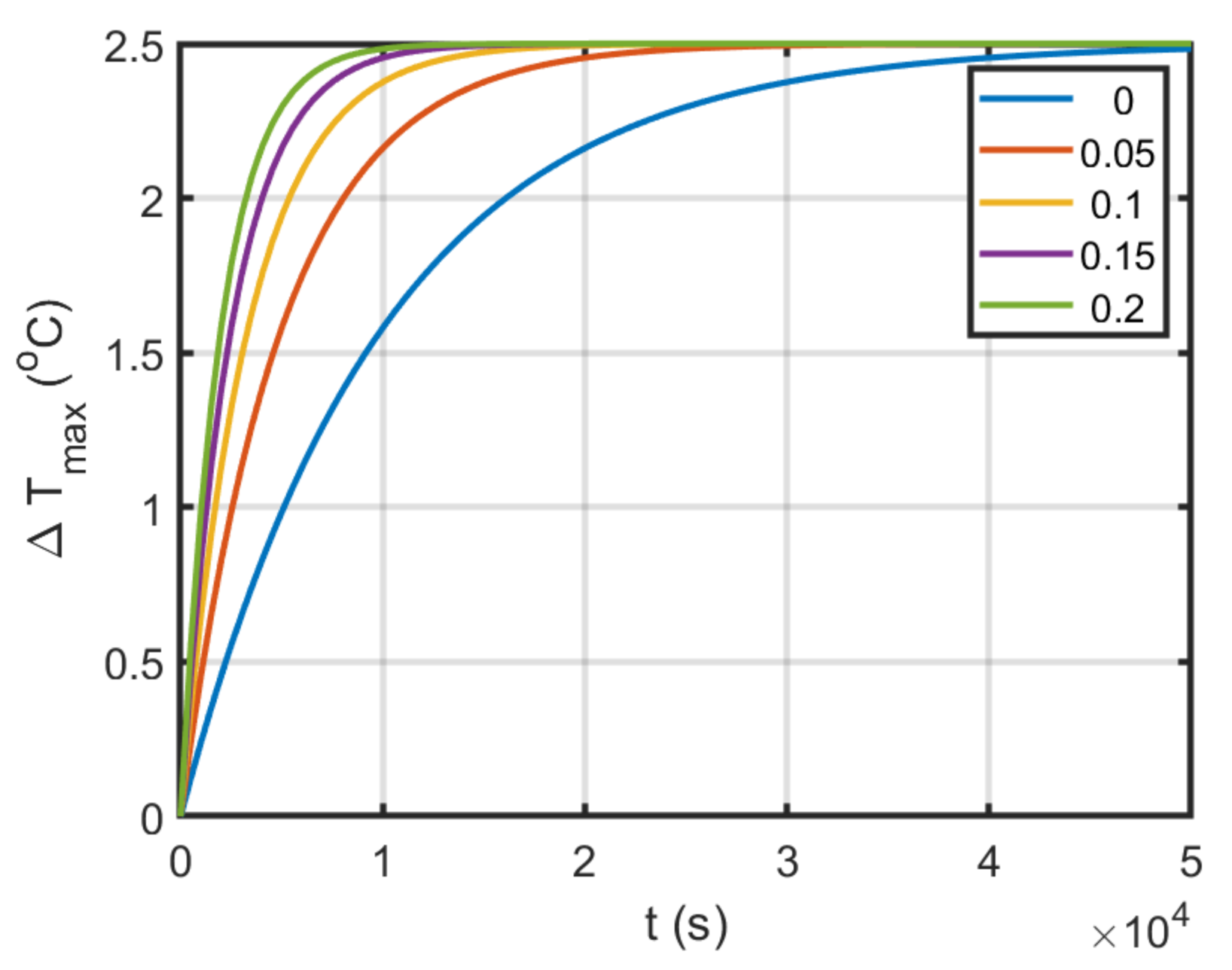
3.3. Fluid and Thermal Analysis

Profile development and contours of velocity magnitude distribution in the liquid part of the PCM cell are plotted in Figure 21. As shown, the liquid profile is developed fast near the initial condition as the absorbed heat in the PCM is converted to phase change in the liquid–solid boundary. Figure 21 does not have a color legend and is focused on showing the melting profile development. In the red zone, the velocity magnitude is maximum while in blue zones (near walls) the velocity magnitude is near zero. As time goes on, the melting process developed in the PCM box. As shown, the velocity is minimum near walls and is maximum at the middle of two flow channels created horizontally at the PCM cell. Detailed velocity distribution in PCM cell with cooling at the end of melting process is plotted in Figure 22. As shown in velocity vectors and magnitude in the PCM field, the maximum velocity happens at the middle of two flow channels with the horizontal direction. At the end of the flow stream, it turns vertically to turn inside by natural convection.

The power distribution inside BAW slab for first and second mode are plotted in Figure 23. The distribution is axially and matches the analytic solution given in Appendix A.

The temperature distribution inside BAW slab for first and second mode are plotted in Figure 24. The distribution is axially and for the case of constant temperature BC at both sides.

Temperature difference ($\Delta T=T-T_{\infty }$) contours are plotted in Figure 25. Figure 25 does not have a color legend and is focused on showing the melting profile development. In the red zone, the velocity magnitude is maximum while in blue zones (near walls) the velocity magnitude is near zero. The figure shows the temperature profiles through the time for various BC. The initial condition of PCM cell is temperature equals the environmental temperature ($T=T_{\infty }$). As time goes on, the cold zone is shortened through the volume, and the heated zone expands. If both sides are kept at environmental temperature the temperature profile inside the slab is parabolic. The case of constant temperature BC at both sides happens when the periodic structure of the BAW + PCM cell forced the melting temperature at both side until the end of phase change. The case of adiabatic BC at the left happens when each BAW + PCM cell is considered as an isolated domain from the other. Such conditions force the melting temperature on the right side until the end of phase change while adiabatic condition at the left of the cell. As shown, the periodic structure causes less temperature increase.

Temperature distribution inside BAW + PCM cell is illustrated in Figure 26. Time dependency of the temperature in the BAW + PCM cell shows that, by considering PCM, the thermal inertia happens in the system.

The effect of nanoparticle concentration on time dependency of maximum temperature is illustrated in Figure 27. By increasing the nanoparticle the rate of interface convection increased and faster phase change happens.

4. Conclusions

In this paper, a FEM code is introduced for the mathematical arrangement of the electro–elastic conditions that oversee the directly constrained vibrations of piezoelectric media. A consonant time reliance is accepted. Both of the methodologies, that of taking care of the field issue (consonant investigation) and that of taking care of the relating eigenvalue issue (modular examination), are portrayed. A FEM programming bundle has been made without any preparation. Significant angles fundamental to the proficient execution of FEM are clarified, for example, the memory of the executives and tackling the summed up piezoelectric eigenvalue issue. Calculations for diminishing the necessary PC memory through enhancement of the framework profile, just as Lanczos calculation for the arrangement of the eigenvalue issue are connected into the product from outer mathematical libraries. Current FEM programming is applied to nitty-gritty mathematical demonstrating of thin-film bulk acoustic wave (BAW) composite resonators. Correlation of results from 2D and full 3D recreations of a resonator is introduced. Specifically, 3D reproductions are utilized to explore the impact of the top terminal shape on the resonator electrical reaction. The legitimacy of the displaying strategy is shown by contrasting the recreated and estimated removal profiles at a few frequencies. The outcomes show that valuable data on the exhibition of the flimsy film resonators can be acquired even with generally coarse cross-sections and, subsequently, moderate computational assets. To highlight the advantages and disadvantages of using NEPCM for cooling application of BAW resonator it is good to notice that when comparing the current devised solution with other solutions from the scientific literature, the efficiency of the current design is more clear. While in common circuits the heat is removed from the semiconductor by conduction to support or with convection or radiative heat transfer modes to the environment, here the phase change plays the role of the heat sink with more thermal inertia. As well, the use of nanoparticles facilitates the heat removal, and also decreases the delay time and thermal inertia of the cooling system. As it would be useful to add information on further research of the authors related to the continuation of this research topic, future research could be conducted to consider the 3D design of a thin-film bulk acoustic wave composite resonators in conjunction with another electrical part to see the effectiveness of current study in an engineering case.

References

1. Abdollahzadeh Jamalabadi, M.Y. Rational Design Calculation of Surface Acoustic Wave Gas Sensor. Phys. J. 2020, 6, 63–87. [Google Scholar]
2. Abdollahzadeh Jamalabadi, M.Y.; Park, J.H. Investigation of Property Variations on Freezing of PCM Containing Nanoparticles. World Appl. Sci. J. 2014, 32, 672–677. [Google Scholar]
3. Makkonen, T.; Pensala, T.; Vartiainen, J.; Knuuttila, J.V.; Kaitila, J.; Salomaa, M.M. Estimating materials parameters in thin-film BAW resonators using measured dispersion curves. IEEE Trans. Ultrason. Ferroelectr. Freq. Control 2004, 51, 42. [Google Scholar] [CrossRef]
4. Abdollahzadeh Jamalabadi, M.Y.; Park, J.H. Effects of Brownian motion on freezing of PCM containing nanoparticles. Therm. Sci. 2016, 20, 1533–1541. [Google Scholar] [CrossRef] [Green Version]
5. Abdollahzadeh Jamalabadi, M.Y. MD Simulation of Brownian Motion of Buckminsterfullerene Trapping in nano-Optical Tweezers. Int. J. Opt. Appl. 2015, 5, 161–167. [Google Scholar]
6. Abdollahzadeh Jamalabadi, M.Y. Use of Nanoparticle Enhanced Phase Change Material for Cooling of Surface Acoustic Wave Sensor. Fluids 2021, 6, 31. [Google Scholar] [CrossRef]
7. Singh, R.P.; Sze, J.Y.; Kaushik, S.C.; Rakshit, D.; Romagnoli, A. Thermal performance enhancement of eutectic PCM laden with functionalised graphene nanoplatelets for an efficient solar absorption cooling storage system. J. Energy Storage 2021, 33, 102092. [Google Scholar] [CrossRef]
8. Sarbu, I.; Sebarchievici, C. A comprehensive review of thermal energy storage. Sustainability 2018, 10, 191. [Google Scholar] [CrossRef] [Green Version]
9. Khan, Z.; Khan, Z.; Ghafoor, A. A review of performance enhancement of PCM based latent heat storage system within the context of materials, thermal stability and compatibility. Energy Convers. Manag. 2016, 115, 132–158. [Google Scholar] [CrossRef]
10. Jiang, Z.Y.; Qu, Z.G. Lithium-ion battery thermal management using heat pipe and phase change material during discharge—Charge cycle: A comprehensive numerical study. Appl. Energy 2019, 242, 378–392. [Google Scholar] [CrossRef]
11. Tariq, S.L.; Ali, H.M.; Akram, M.A.; Janjua, M.M.; Ahmadlouydarab, M. Nanoparticles enhanced phase change materials (NePCMs)-A recent review. Appl. Therm. Eng. 2020, 176, 115305. [Google Scholar] [CrossRef]
12. Raj, C.R.; Suresh, S.; Singh, V.K.; Bhavsar, R.R.; Chandrasekar, M.; Archita, V. Life cycle assessment of nanoalloy enhanced layered perovskite solid-solid phase change material till 10000 thermal cycles for energy storage applications. J. Energy Storage 2021, 35, 102220. [Google Scholar] [CrossRef]
13. Tiari, S.; Hockins, A.; Mahdavi, M. Numerical study of a latent heat thermal energy storage system enhanced by varying fin configurations. Case Stud. Therm. Eng. 2021, 25, 100999. [Google Scholar] [CrossRef]
14. Tiari, S.; Mahdavi, M. Computational study of a latent heat thermal energy storage system enhanced by highly conductive metal foams and heat pipes. J. Anal. Calorim. 2020, 141, 1741–1751. [Google Scholar] [CrossRef]
15. Li, W.Q.; Guo, S.J.; Tan, L.; Liu, L.L.; Ao, W. Heat transfer enhancement of nano-encapsulated phase change material (NEPCM) using metal foam for thermal energy storage. Int. J. Heat Mass Transf. 2021, 166, 120737. [Google Scholar] [CrossRef]
16. Dutkowski, K.; Kruzel, M.; Zajączkowski, B. Determining the heat of fusion and specific heat of microencapsulated phase change material slurry by thermal delay method. Energies 2021, 14, 179. [Google Scholar] [CrossRef]
17. Abdulateef, A.M.; Jaszczur, M.; Hassan, Q.; Anish, R.; Niyas, H.; Sopian, K.; Abdulateef, J. Enhancing the melting of phase change material using a fins–nanoparticle combination in a triplex tube heat exchanger. J. Energy Storage 2021, 35, 102227. [Google Scholar] [CrossRef]
18. Nie, C.; Liu, J.; Deng, S. Effect of geometric parameter and nanoparticles on PCM melting in a vertical shell-tube system. Appl. Therm. Eng. 2021, 184, 116290. [Google Scholar] [CrossRef]
19. Aqib, M.; Hussain, A.; Ali, H.M.; Naseer, A.; Jamil, F. Experimental case studies of the effect of Al2O3 and MWCNTs nanoparticles on heating and cooling of PCM. Case Stud. Therm. Eng. 2020, 22, 100753. [Google Scholar] [CrossRef]
20. Khatibi, M.; Nemati-Farouji, R.; Taheri, A.; Kazemian, A.; Ma, T.; Niazmand, H. Optimization and performance investigation of the solidification behavior of nano-enhanced phase change materials in triplex-tube and shell-and-tube energy storage units. J. Energy Storage 2021, 33, 102055. [Google Scholar] [CrossRef]
21. Maher, H.; Rocky, K.A.; Bassiouny, R.; Saha, B.B. Synthesis and thermal characterization of paraffin-based nanocomposites for thermal energy storage applications. Therm. Sci. Eng. Prog. 2021, 22, 100797. [Google Scholar]
22. Chen, G. Nanoscale Energy Transport and Conversion: A Parallel Treatment of Electrons, Molecules, Phonons, and Photons; Oxford University Press: Oxford, UK, 2005; ISBN 9780195159424. [Google Scholar]
23. Santhosh, S.; Satish, M.; Yadav, A.; Anish Madhavan, A. Thermal analysis of Fe2O3—Myristic acid nanocomposite for latent heat storage. Mater. Today Proc. 2021, 52, 687. [Google Scholar]
24. U Mekrisuh, K.; Giri, S.; Udayraj; Singh, D.; Rakshit, D. Optimal design of the phase change material based thermal energy storage systems: Efficacy of fins and/or nanoparticles for performance enhancement. J. Energy Storage 2021, 33, 102126. [Google Scholar] [CrossRef]
25. Hosseinzadeh, K.; Erfani Moghaddam, M.A.; Asadi, A.; Mogharrebi, A.R.; Jafari, B.; Hasani, M.R.; Ganji, D.D. Effect of two different fins (longitudinal-tree like) and hybrid nano-particles (MoS2-TiO2) on solidification process in triplex latent heat thermal energy storage system. Alex. Eng. J. 2021, 60, 1967–1979. [Google Scholar] [CrossRef]
26. Nakhchi, M.E.; Hatami, M.; Rahmati, M. A numerical study on the effects of nanoparticles and stair fins on performance improvement of phase change thermal energy storages. Energy 2021, 215, 119112. [Google Scholar] [CrossRef]
27. Li, F.; Almarashi, A.; Jafaryar, M.; Hajizadeh, M.R.; Chu, Y.-M. Melting process of nanoparticle enhanced PCM through storage cylinder incorporating fins. Powder Technol. 2021, 381, 551–560. [Google Scholar] [CrossRef]
28. Yu, Q.; Zhang, C.; Lu, Y.; Kong, Q.; Wei, H.; Yang, Y.; Gao, Q.; Wu, Y.; Sciacovelli, A. Comprehensive performance of composite phase change materials based on eutectic chloride with SiO2 nanoparticles and expanded graphite for thermal energy storage system. Renew. Energy 2021, 172, 1120–1132. [Google Scholar] [CrossRef]
29. Fang, Y. A Comprehensive Study of Phase Change Materials (PCMs) for Building Wall Applications. Ph.D. Dissertation, University of Kansas, Lawrence, KS, USA, 2009. [Google Scholar]
Figure 1. Schematic of piezoelectric and electrodes in a BAW configuration.
Magnetochemistry 07 00144 g001
Figure 2. Geometry of the BAW resonator assisted by PCM box in 2D simulation.
Magnetochemistry 07 00144 g002
Figure 3. Schematic of BAW piezoelectric material (ZnO) and periodic condition (for real and imaginary k), terminal, and ground boundary condition at aluminum surfaces.
Magnetochemistry 07 00144 g003
Figure 4. Validation of fluid part by comparing the solid percent of PCM versus time in a melting process.
Magnetochemistry 07 00144 g004
Figure 5. Geometrical parameters for the case of heat generation in a slab.
Magnetochemistry 07 00144 g005
Figure 6. Heat generation in axial direction calculated by FEM and analytical solution.
Magnetochemistry 07 00144 g006
Figure 7. Accumulated charge on electrode as a function of frequency estimated by FEM and ANSYS.
Magnetochemistry 07 00144 g007
Figure 8. Admittance as a function of frequency estimated by FEM and Makkonen et al. [3].
Magnetochemistry 07 00144 g008
Figure 9. Eigenfrequency, participation factors, and effective modal masses of the first six modes of BAW piezoelectric in eigenfrequency evaluation.
Magnetochemistry 07 00144 g009
Figure 10. Horizontal displacement of mode 1.
Magnetochemistry 07 00144 g010
Figure 11. Vertical displacement of mode 1.
Magnetochemistry 07 00144 g011
Figure 12. Horizontal displacement of mode 2.
Magnetochemistry 07 00144 g012
Figure 13. Vertical displacement of mode 2.
Magnetochemistry 07 00144 g013
Figure 14. Horizontal displacement of mode 3.
Magnetochemistry 07 00144 g014
Figure 15. Vertical displacement of mode 3.
Magnetochemistry 07 00144 g015
Figure 16. Damping ratio (blue dashed-line) and quality factor (red line) as a function of frequency.
Magnetochemistry 07 00144 g016
Figure 17. Quality factor for frequency as a function of frequency.
Magnetochemistry 07 00144 g017
Figure 18. Real part (blue line) and imaginary part (red dashed-line) of scattering parameter as a function of frequency.
Magnetochemistry 07 00144 g018
Figure 19. Dispersion curve for imaginary wave numbers (evanescent waves) and for real wave numbers (propagating waves).
Magnetochemistry 07 00144 g019
Figure 20. Total power dissipation as a function of frequency.
Magnetochemistry 07 00144 g020
Figure 21. Profile development and contours of velocity magnitude in liquid part of PCM cell (a) t = 10, (b) t = 100, (c) t = 200, (d) t = 500, (e) t = 1000, (f) t = 2000, (g) t = 5000, (h) t = 10,000.
Magnetochemistry 07 00144 g021
Figure 22. Velocity vectors and magnitude in PCM field.
Magnetochemistry 07 00144 g022
Figure 23. Power distribution inside BAW slab for first and second mode.
Magnetochemistry 07 00144 g023
Figure 24. Temperature distribution inside BAW slab for first and second mode.
Magnetochemistry 07 00144 g024
Figure 25. Temperature profiles inside liquid part of PCM cell (a) constant temperature BC at the both sides, (b) maximum temperature while constant temperature BC at the both sides, (c) adiabatic BC at the left, (d) maximum temperature while adiabatic BC at the left.
Magnetochemistry 07 00144 g025
Figure 26. Temperature distribution inside BAW + PCM cell (a) profile plot (b) surface plot.
Magnetochemistry 07 00144 g026
Figure 27. Effect of nanoparticle concentration on maximum temperature.
Magnetochemistry 07 00144 g027