Article

The Hydrodynamic Behavior of Vortex Shedding behind Circular Cylinder in the Presence of Group Focused Waves

Normandie Université, UNICAEN, UNIROUEN, CNRS, UMR 6143 M2C, 14000 Caen, France
*
Author to whom correspondence should be addressed.
Submission received: 10 November 2021 / Revised: 2 December 2021 / Accepted: 20 December 2021 / Published: 22 December 2021
(This article belongs to the Special Issue Nonlinear Wave Hydrodynamics, Volume II)

Abstract

:
Vortex shedding behind an elastically mounted circular cylinder in the presence of group focused waves propagating upstream was investigated using a classical approach (time series and FFT) and nonclassical approach (complex 2D Morlet wavelets). Wavelet analysis emerged as a novel solution in this regard. Our results include wave trains with different nonlinearities propagating in different water depths and derived from three types of spectra (Pierson–Moskowitz, JONSWAP (γ = 3.3 or γ = 7)). It was found that the generated wave trains could modify regimes of shedding behind the cylinder, and subharmonic frequency lock-in could arise in particular situations. The occurrence of a lock-in regime in the case of wave trains propagating in intermediate water locations was shown experimentally even for small nonlinearities. Moreover, the application of time-localized wavelet analysis was found to be a powerful approach. In fact, the frequency lock-in regime and its duration could be readily identified from the wavelet-based energy and its corresponding ridges.

Graphical Abstract

1. Introduction

Vortex shedding behind cylindrical structures has been the focus of many experimental and numerical studies over recent decades, given its practical importance in the maritime industry [1,2,3,4]. When exposed to highly nonlinear perturbations, vortex shedding provides modifications particularly in the wake around the cylinder. Therefore, these modifications should be considered when evaluating vortex shedding’s disadvantages. The frequency of vortex shedding fsh in the wake depends on the frequency of the perturbation fw. More precisely, there is a fundamental synchronization region in which fsh is controlled by the imposed perturbation, which is referred to as the vortex shedding lock-in regime [5,6]. This regime may occur at frequencies of perturbation fw equal to fsh (harmonic lock-in), 2fsh (subharmonic lock-in), or fsh/n with n = 2, 3, … (superharmonic lock-in) [7]. In the present work, we only focused on subharmonic lock-in regime, i.e., fw~2fsh.
In the global context of climate change evolving the expansion of marine renewable energy and the impacts of storminess on man-induced frames, cylindrical structures should be designed to remain functional in increasingly intermediate and deep-water locations during extreme events. For that reason, it is essential to study vortex shedding around the cylinder in similar harsh environments. In previous studies, several physical mechanisms have been suggested as causing the formation of extreme waves, including dispersive focusing in shallow or intermediate water depth [8,9] and modulation instability in deep-water depth, i.e., kh > 1.363, where k and h are the wavenumber and water depth, respectively [10]. In the present work, we have decided to limit our focus to extreme waves generated by the spatiotemporal wave focusing as a consequence of the dispersive nature of water waves. Dispersive focusing is traditionally used in laboratory modeling [11,12,13] to represent the expected wave profile based on the NewWave theory [14], which describes the wave velocity components and the free surface elevation of a focused group of localized waves. The waves are superposed and brought into phase at one point, generating an extreme wave event. The impact of wave trains on the structure of vortices behind the cylinder has not yet been investigated. Therefore, we will study the features of frequency lock-in of vortex shedding in the wake when the external forcing is due to wave trains.
The most widely used frequency analysis technique to detect the shedding frequency in the wake of a cylinder is the Fast Fourier Transform (FFT) [7]. Given the rapidly changing nature of extreme waves, the reliability of the forecast of extreme waves’ impact on the wake behind the cylinder using FFT is low and hard to temporally expect. Consequently, FFT does not reflect the accurate time localization of the subharmonic frequency lock-in. In this work, we explore the capabilities of the complex wavelet convolution tool to improve the localization of the subharmonic lock-in. The need to evaluate relatively long-term and highly random phenomena using wavelet analysis is already found in a variety of disciplines, such as plasma physics [15], health-related areas like neuroscience [16], geophysics [17], or ocean wave analysis [18,19,20].
Observations of the shedding frequency fsh in the wake of an elastically mounted cylinder subjected to wave trains are presented in this paper. Firstly, a spectral analysis was used in order to investigate the spectral changes in the wake of the cylinder from random wave trains with a wide range of water depth, nonlinearities, and spectra types. Secondly, wavelet analysis was proposed as a tool to identify the temporal evolution of subharmonic frequency lock-in based on the wavelet transform.
The remainder of this paper is organized as follows. Section 2 describes our experimental set-up. Section 3 is devoted to our experimental results and observations. The fourth and last sections present our conclusions and perspectives.

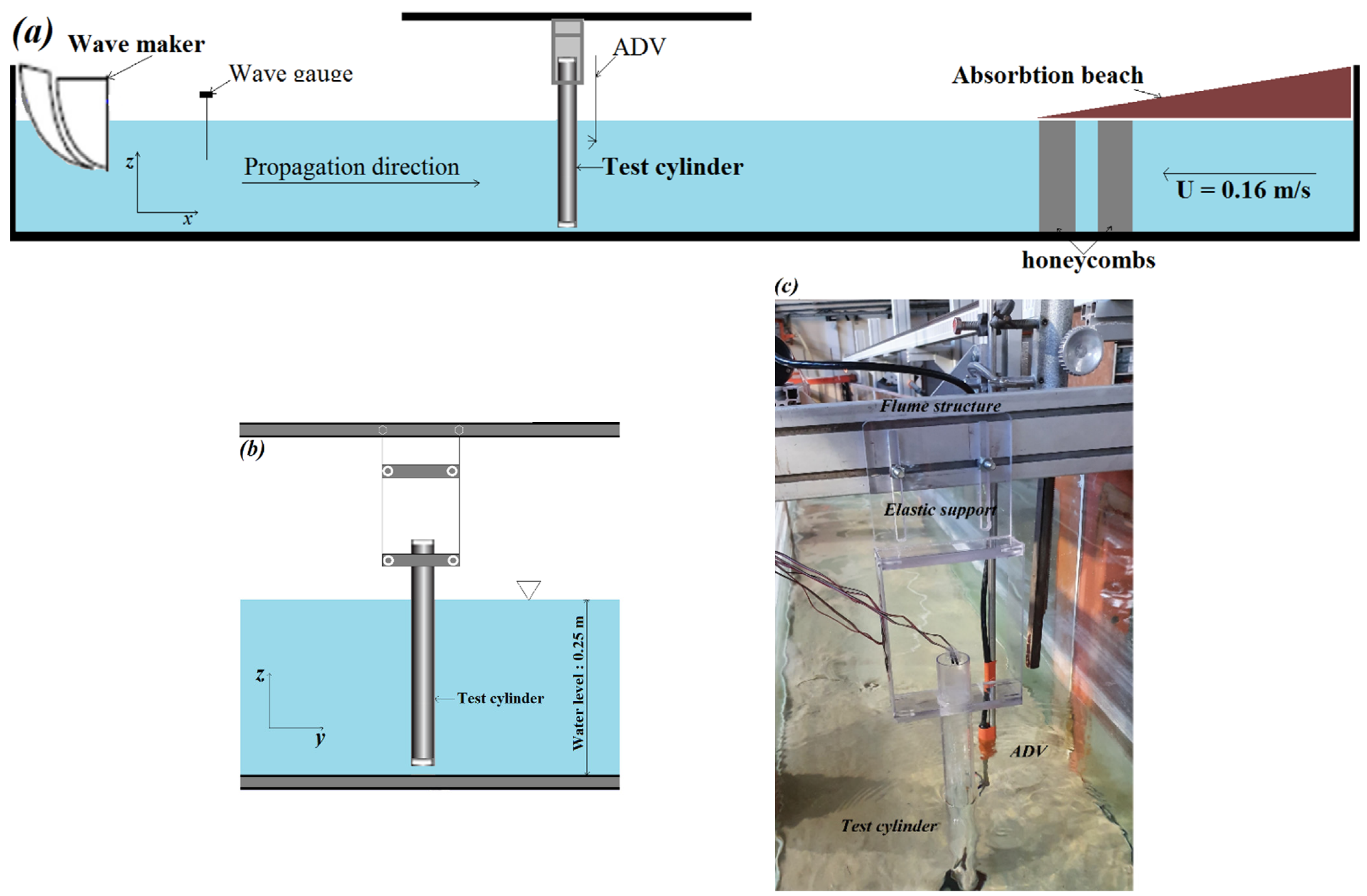
2. Materials and Methods

The tests were conducted at the Morphodynamique Continentale et Côtière de Caen, France. The wave flume was 16 m long, 0.5 m wide, and filled with tap water to a depth of h0 = 0.25 m (Figure 1). A piston-type wave maker was located at one end of the flume to generate wave trains, and a foam absorber beach was at the other end. Two honeycombs of about 20 cm were installed in the flume, as shown in Figure 1a, in order to reduce wave reflection and to minimize the intensity of turbulent fluctuations generated by the pump. Temporal variations of free surface elevation measured at x = 2 m from the wave maker, were recorded by a wave gauge with a sampling rate of 100 Hz. These measurements were used to identify input wave train parameters.
The experimental setup is shown in Figure 1. The rigid circular cylinder model, situated at x = 7 m from the wave maker, was made from Plexiglas with diameter D = 0.04 m and had an immersed length of L = 0.248 m. An acoustic doppler velocimeter (ADV), placed at a distance d ~ D from the cylinder, was used to measure the longitudinal wave velocity Vx upstream the structure. Wave trains propagated on the background of a steady current U = 0.16 m/s, corresponding to a Reynolds number R e = U D ν = 6400 (ν is the kinematic viscosity) and a Froude number F r = U g h 0 = 0.1 . The definition of the flow velocity and the Reynolds and Froude numbers were the same as in Hans et al. (2016). The cylinder was vertically clamped by its upper end to an elastic support, which was fixed on the flume’s structure. The lower end of the cylinder was at approximately 2 mm (5% D) from the flume’s floor (Figure 1b,c).
Focused wave trains were generated with a technique similar to that in [13]. The resulting wave trains were derived from Pierson–Moskowitz, JONSWAP (γ = 3.3), and JONSWAP (γ = 7) spectra. Figure 2 shows three sets of time series of Pierson–Moskowitz, JONSWAP (γ = 3.3), and JONSWAP (γ = 7) wave trains and their corresponding dimensionless frequency spectra.
By adjusting the nonlinearity S0, breaking wave trains with different amplitudes were generated. The focus point was set to x = 12 m > x = 7 m and therefore, all of the generated wave trains broke downstream the cylinder. The nonlinearity parameter S 0 = k S 0 i = 1 n a i , also called local wave steepness, was the same as S0 in [13]. Here, k S 0 was the characteristic wavenumber, and ai was the amplitude of the ith wave component. The nonlinearity parameter S0 was calculated at x = 2 m from the wave maker. The generated wave trains propagated in intermediate water depth (0.9 < kwh0 < 2.04). Table 1, Table 2 and Table 3 present some key parameters of the generated wave trains, which were categorized via their spectra, wave nonlinearity S0, and the water depth kwh0. One hundred and twenty crest-focused wave groups were generated in this study.

3. Results and Discussions

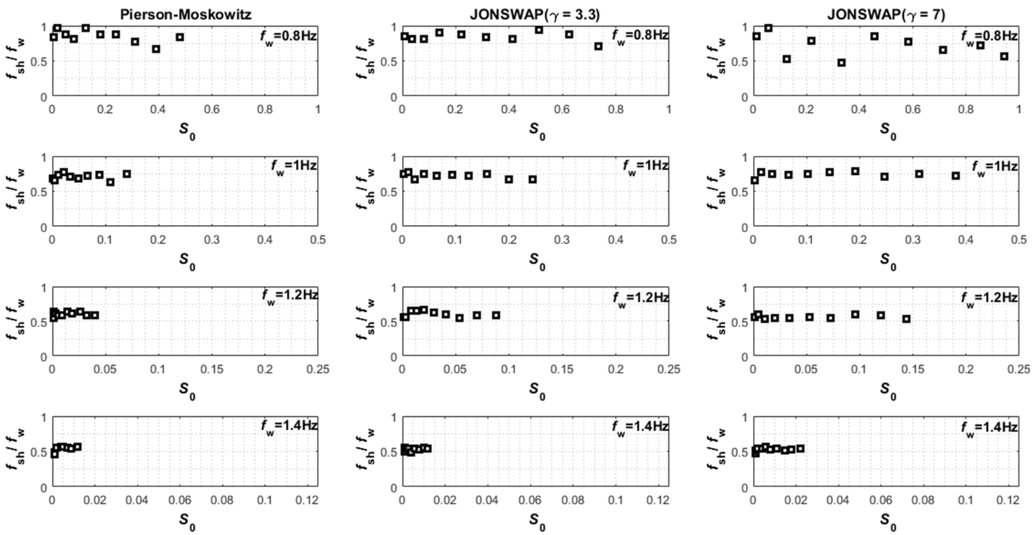
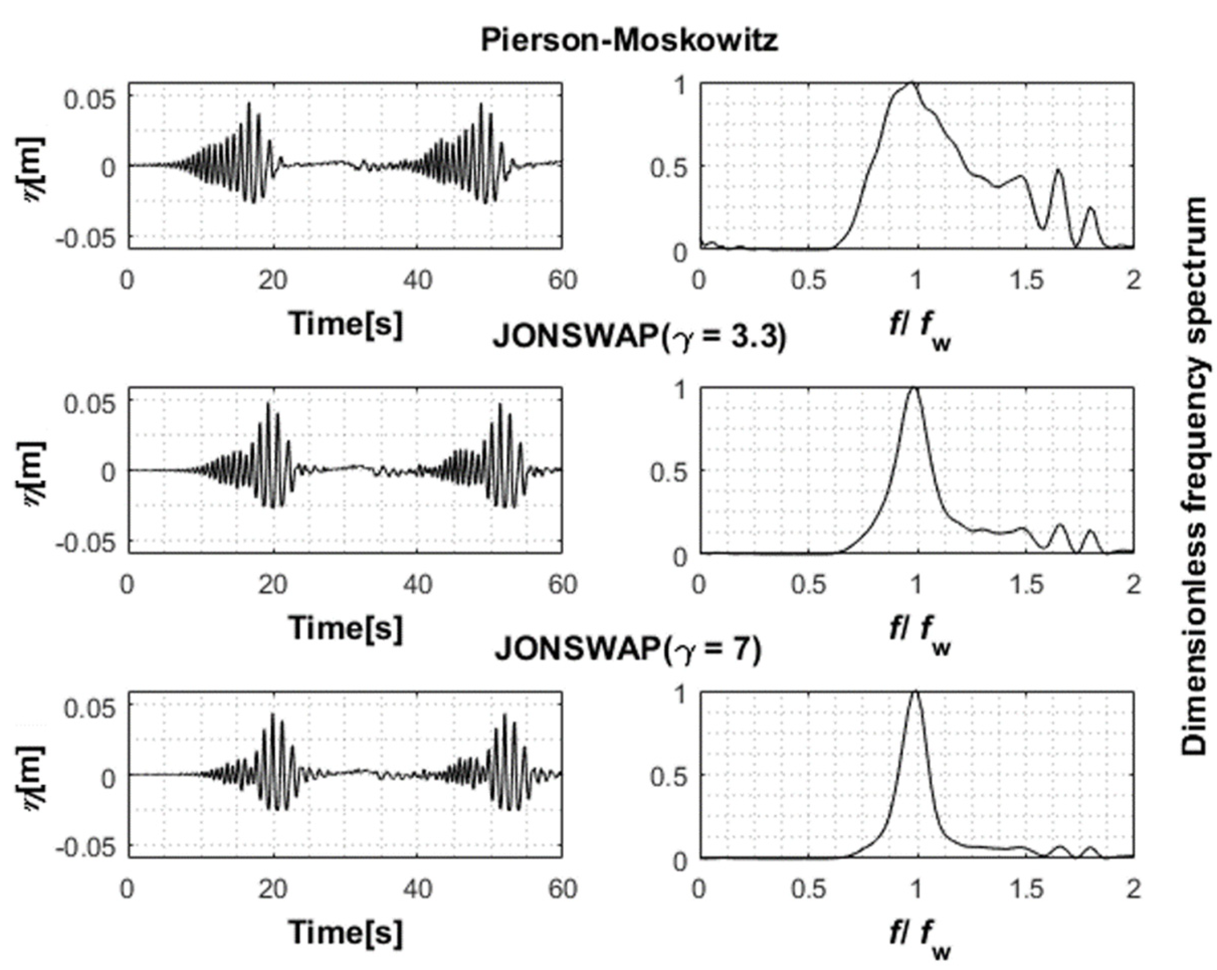
3.1. Fourier Analysis

The longitudinal velocity Vx measured downstream the cylinder and FFT analysis were used in order to obtain the velocity energy spectrum   S   ( V x ( t ) ) = 2   | F ( V x ( t ) ) | ² . Here, F was the Fourier transform of the flow velocity Vx. The sampling time for ADV measurements was truncated to 187.5 s, corresponding to 37,500 points. The lower and the upper cut-off frequencies were set, respectively, to 0.5 Hz and 2fw. Outside this frequency range, the spectral energy was very low (less than 2% of the total energy) and could be neglected. The data for this paper are available in the Supplementary Materials.
Figure 3 exhibits a typical set of velocity spectra for twelve wave trains having approximately the same nonlinearity S0, derived from the three spectra and propagating in four different water depths. For each spectrum, the amplitude was normalized by the maximum of the spectral energy, and the shedding frequency fsh was normalized by the wave train peak frequency fw. The ratio fsh/fw and the spectrum width were used as indicators for detecting the subharmonic synchronization regime. In Hans et al. (2016), a spectral width of less than 3% of fsh/fw = 0.5 was used, in the case of regular waves, as a criterion by which it is possible to know if the frequency lock-in occurred or not. In this study, the presence of a subharmonic-like regime was characterized by fsh/fw = 0.5 and a spectrum width Δf = 10% of fsh/fw = 0.5, in which more than 90% of the total energy was present.
As the water depth increased, decreasing shedding frequency was featured, and the energy accumulation near f = fw/2 was evident. The existence of the subharmonic-like regime narrowed the high and low amplitude range of the velocity spectra. The shedding frequency and the wave peak frequency subsynchronized at kwh0 > 2.04, while the FFT spectra of the ADV signal were broad-banded with peak frequencies higher than fsh/fw = 0.5 in shallower water depths kwh0 < 2.04.
The dominant frequency of longitudinal velocity fluctuations in the wake fsh measured for all the studied wave trains is summarized in Figure 4. One can observe that the wave nonlinearity S0 and the spectrum type had no noticeable impact on the behavior of the shedding frequency evolution versus the steepness.

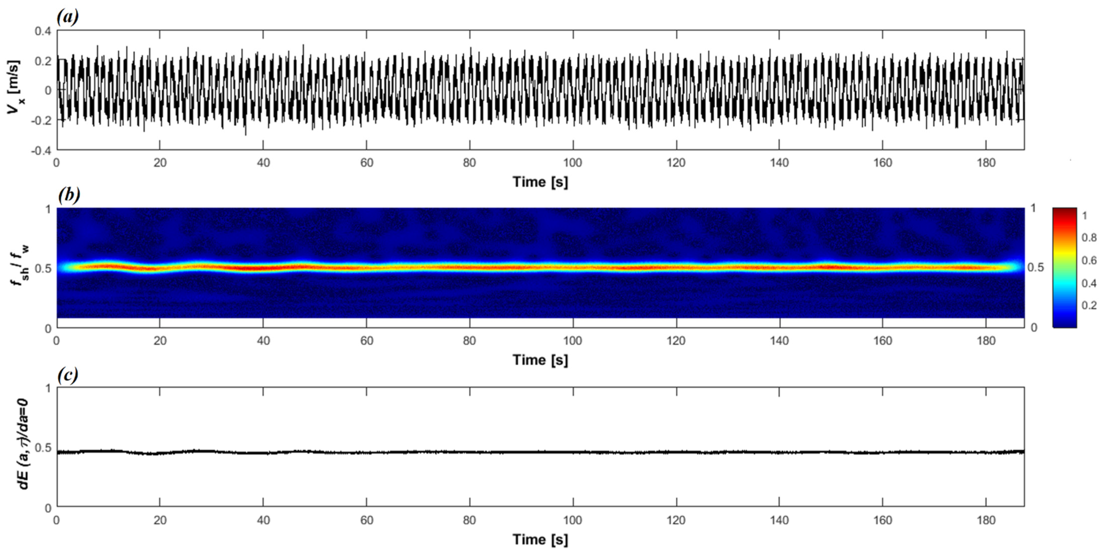
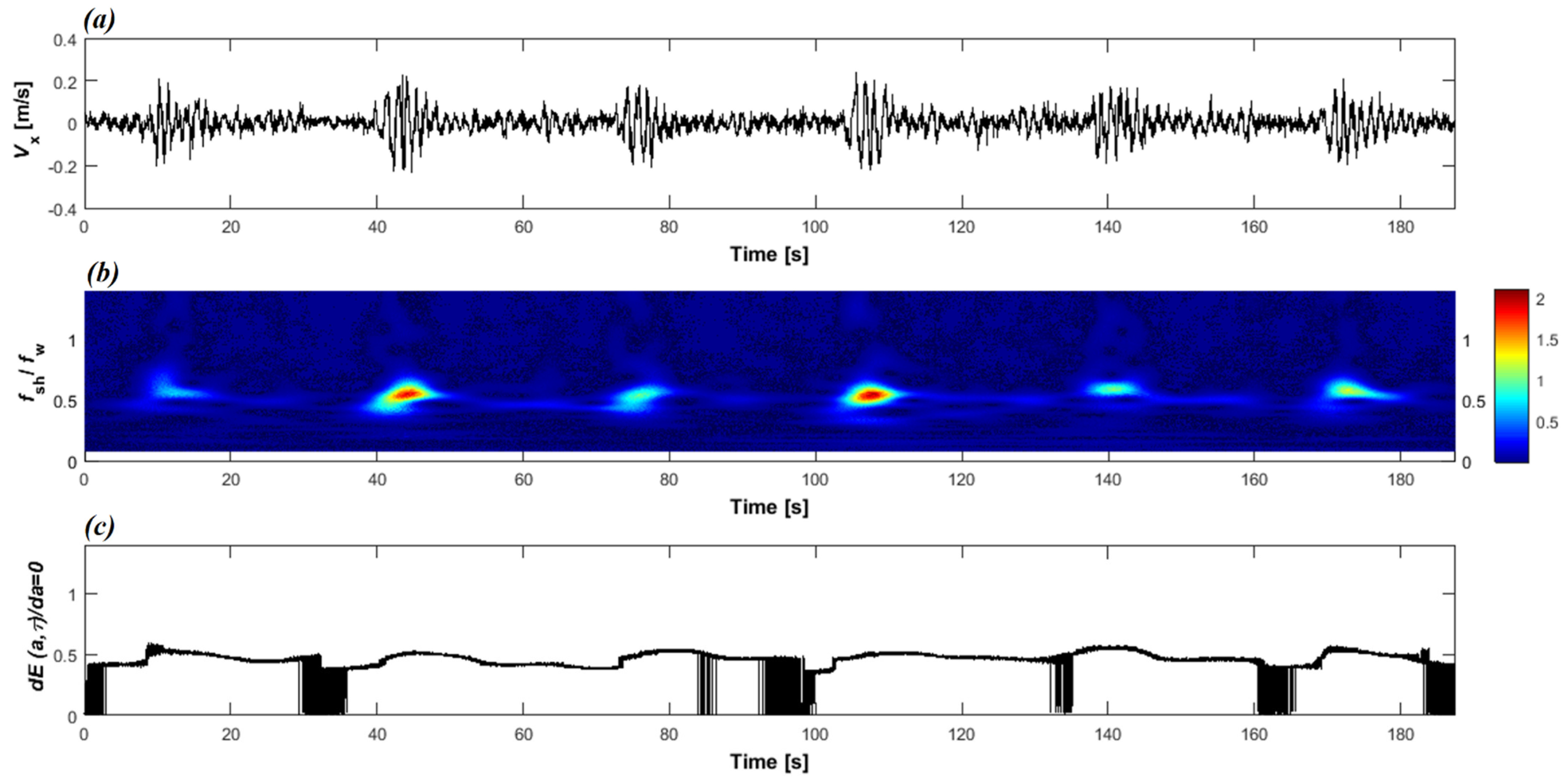
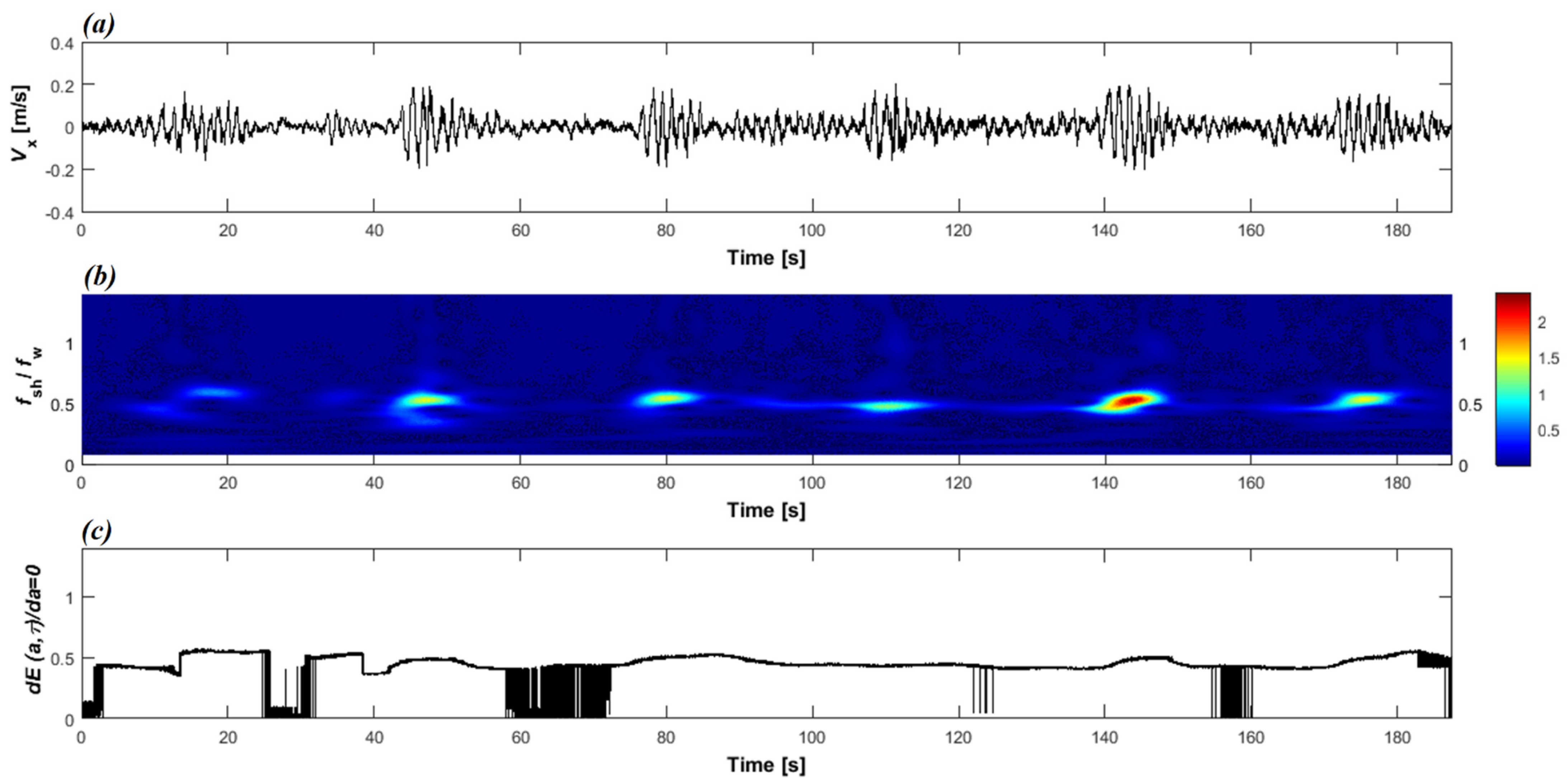
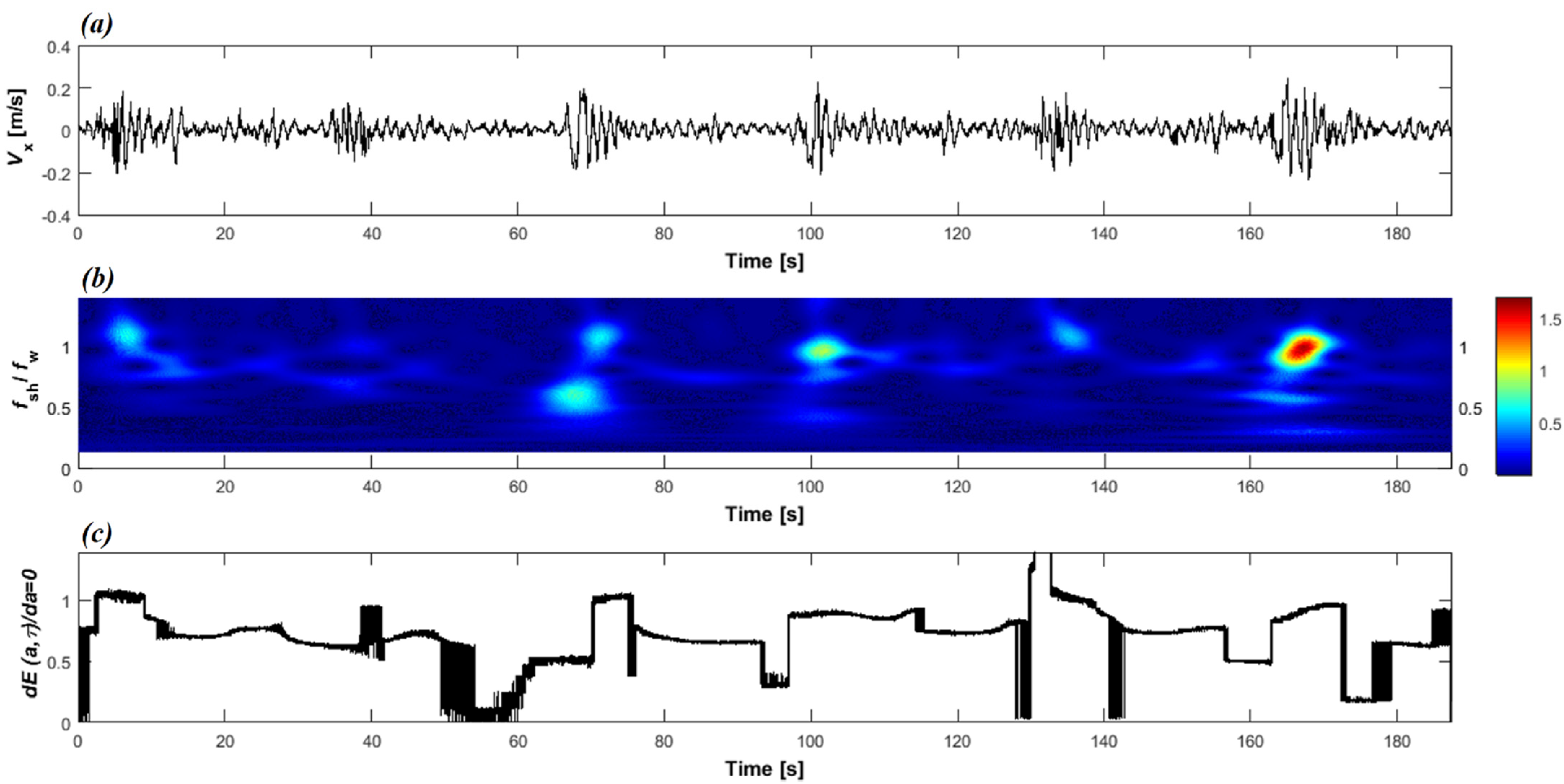
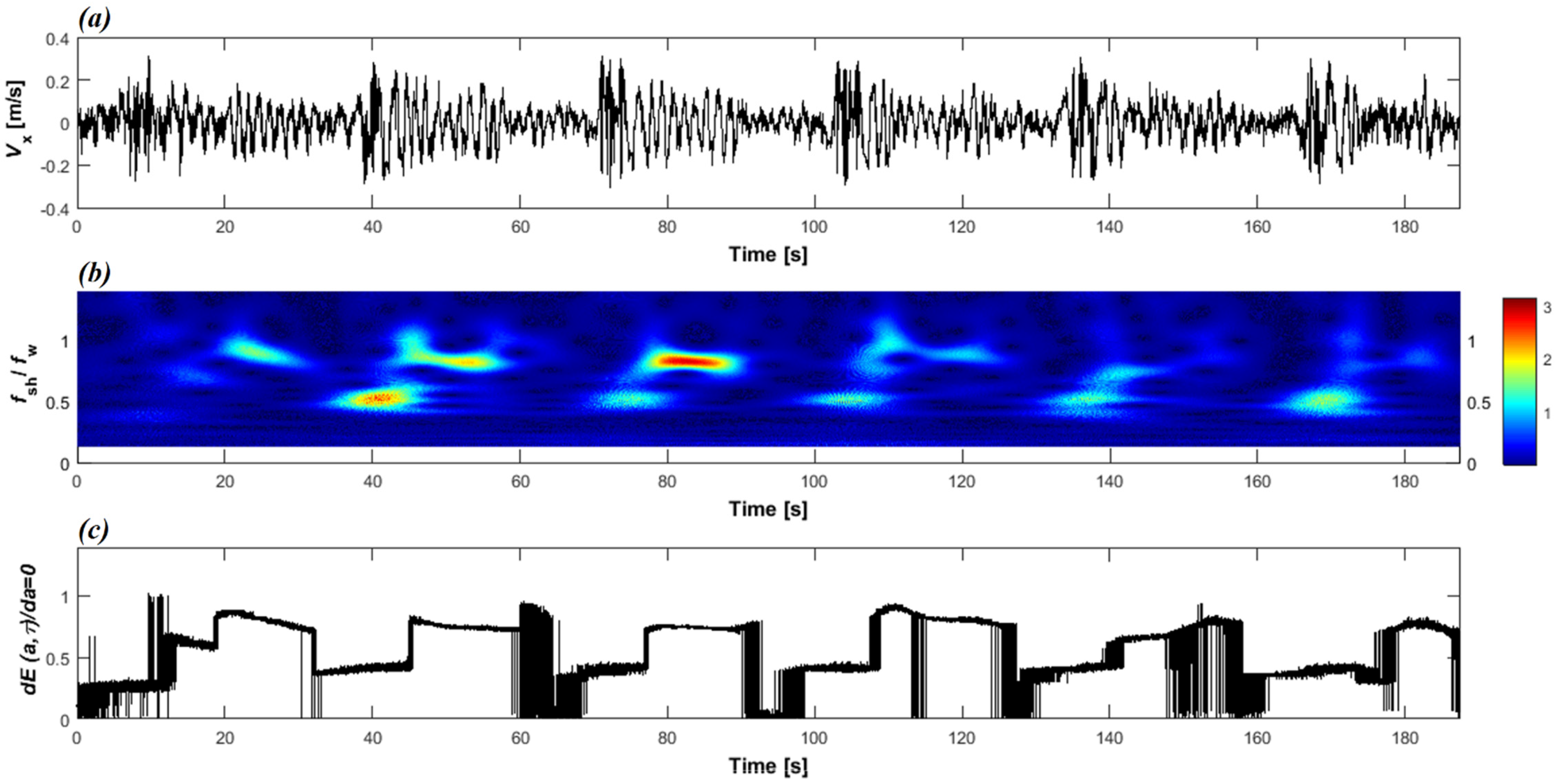
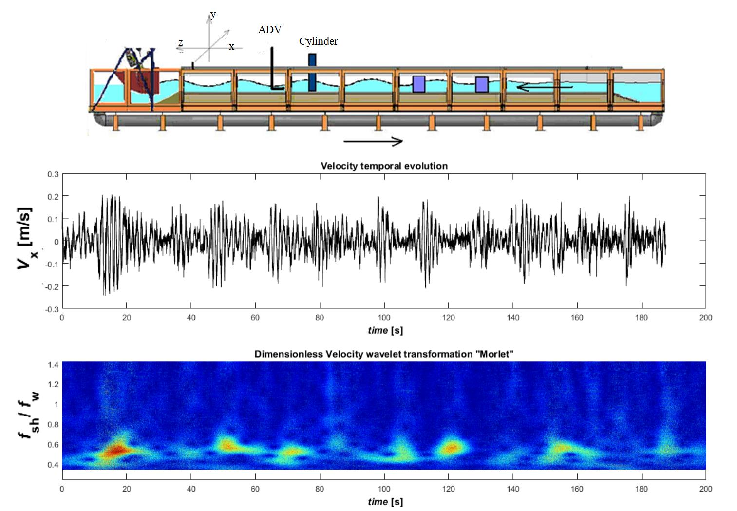
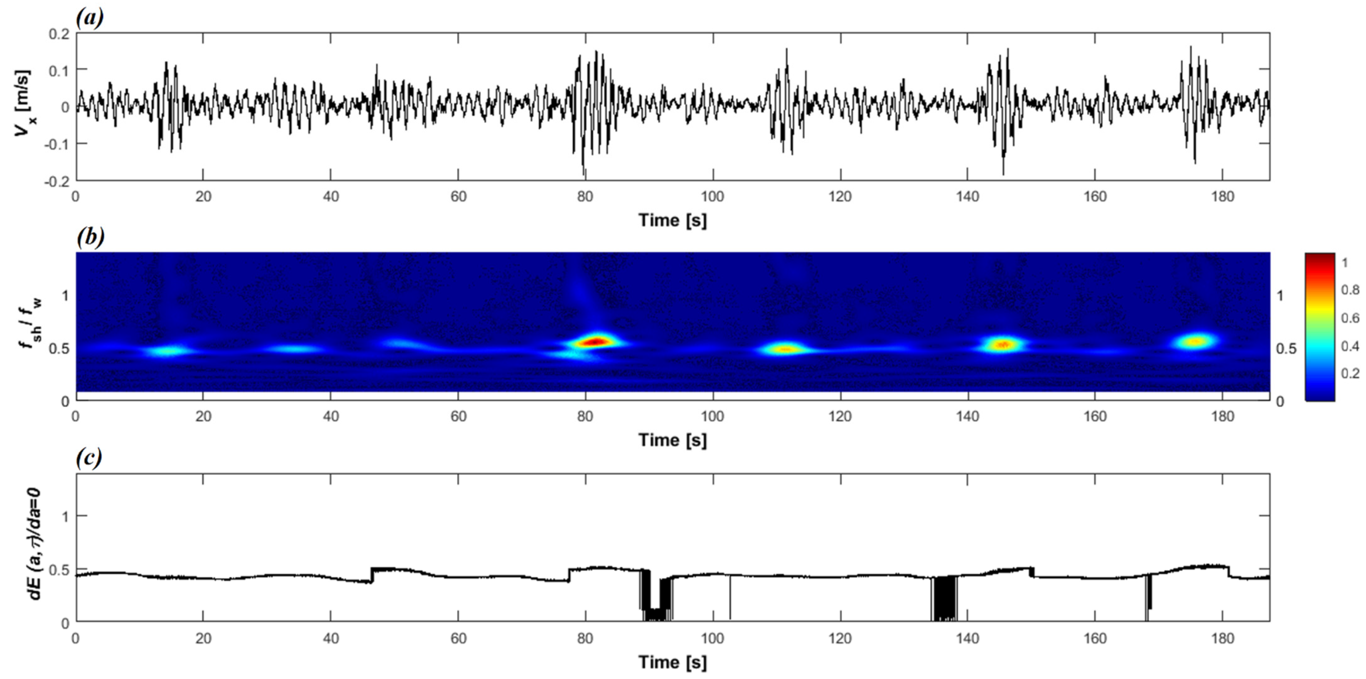
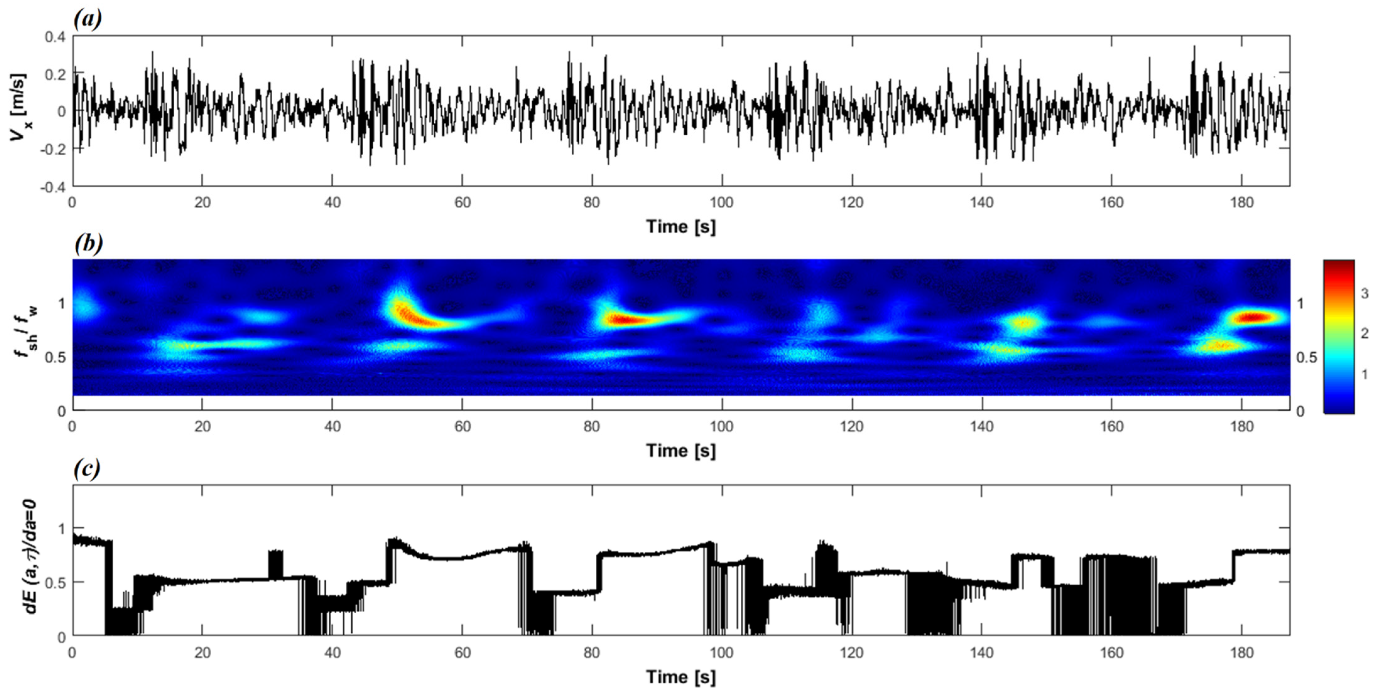
3.2. Wavelet Analysis

The spectral method used in the last section did not take into account signals whose constituent frequencies varied over time. Consequently, we needed a tool that has high resolution in the frequency and time domain, allowing us to identify at which frequencies the signal oscillated, and most importantly, at which time they occurred [21]. To efficiently and accurately detect frequency lock-in in the wake of the cylinder, the wavelet transform was proposed. Among all tests, the experimental results of six representative cases are provided in Table 4. It is important to note that similar results were obtained for the remaining wave trains.
The continuous wavelet transform WT (a,τ) of the ADV temporal signal Vx (t) was defined as a convolution integral of Vx (t) with dilated and scaled versions of a so-called mother wavelet ψ     a , τ * [22,23]:
W T   ( a , τ ) = + V x   ( t )   ψ     a , τ   * d t
The asterisk indicates the complex conjugate, and ψa,τ represents the so-called mother wavelet function dilated by a factor τ and scaled by a factor a. Informally, Vx(t) × ψa,τ represents the energy of the ADV temporal signal around time t in the frequency band centered at 2i. Hence, scales can be written as fractional powers of two [23]:
a i = a 0 2 i δ ,   i = 1 ,   2 ,   3 M
M = 1 δ l o g 2 ( N Δ t a 0 )
where a0 = 0.01 is the smallest resolvable scale, M denotes the largest scale, and δ is the scale factor. The increase of the scale a is equivalent to moving the frequency content of the mother wavelet towards lower frequencies. However, the decrease of a is equivalent to moving its frequency content towards higher frequencies. We opted for a scale factor δ = 0.005, giving a total of 380 frequencies. The time sampling and the number of points were, respectively, Δt = 0.005 s and N = 37,500.
The wavelet transform WT (a,τ) can be displayed on a 2D frequency versus time color plot, with the colors representing the magnitudes of WT (a,τ). Abrupt changes in the temporal signal affect the values of WT (a,τ) at all scales and can be easily detected. As our wavelet transform was complex-valued, it could be expressed in terms of the modulus |WT (a,τ)|, which can be interpreted as the wavelet energy spectrum (i.e., scalogram). The magnitude of WT (a,τ) characterizes the occurrence and the intensity of the counterpart time scale at given time t. Consequently, the energy density of the signal Vx (t) in the time scale plan could be estimated by:
E ( a , τ ) = | W T   ( a , τ ) | ²
Wavelet analysis offers a large choice in the form of mother wavelets to represent the temporal signal as compared to cosines and sines used in the Fast Fourier Transform (FFT) and Short-Time Fourier Transform (STFT). The wavelet-based energy of the Mexican hat [24], Daubechies [25], Shannon [26], and Morlet [20,21,27] mother wavelets for the time series of the velocity signal Vx resulting from the propagation of a JONSWAP (γ = 7) wave train (Case 120) are presented in Figure 5. The shapes of E (a,τ) were qualitatively similar when using different mother wavelets. Compared to the Morlet wavelet, more irregularities in E (a,τ) based on the Mexican hat, Daubechies, and Shannon mother wavelets were found, and smoothing operations may be needed to investigate frequencies present in the wavelet spectrum. Consequently, the Morlet mother wavelet was selected to be the most suitable for our purpose. The complex Morlet wavelet, also called the Gabor wavelet, can be interpreted as a sine wave tapered by a Gaussian window:
ψ ( t ) = 1 π ν 0 e t 2 ν 0 e j 2 π ω 0 t
where ν0 is the bandwidth and ω0 is the center frequency. A wider Morlet provides a weak temporal precision but good spectral precision, and vice versa for a narrower Morlet [28]. Obviously, the wavelet energy of the signal in the time scale plan was calculated for wavelets with different center frequencies ω0 (namely 1, 1.5, 2, 2.5, 3, 3.5, 4, 4.5, 5, 5.5, and 6). For the signal decomposition, the maximum of the wavelet energy was used as an indicator for selecting the optimal center frequency ω0 [29]. When ω0 = 3 for most of the studied wave signals, the maximum of energy was obtained. Thus, the number three is the optimum frequency of the mother wavelet for signal decomposition. Concerning the bandwidth ν0, it was fixed to 1 for real-time requirement and simplicity.
Additionally, it can be useful to plot local maxima in the two-dimensional representation of wavelet information. These maxima, also called wavelet ridges, represent those locations in the time-frequency plan and are useful for pinpointing important frequencies at a given time t [21,28]. In addition to the energy wavelet density E (a,τ), to simplify its visualization, the dynamics of the local maxima (i.e., the time evolution of the wavelet ridges) can be calculated as follows:
E   ( a , τ ) a = 0
Figure 6 exhibits a simple illustration of the wavelet-based spectrum of the longitudinal velocity Vx in the presence of a sine wave with a frequency f = 1.35 Hz. Hans et al. [7] demonstrated that this wave belongs to the subharmonic lock-in region. Figure 6b shows a noticeable energetic band centered at fsh/fw = 0.5, which means that the subharmonic lock-in was continuously present. Figure 6c shows that the associated wavelet ridges were almost constant, i.e., dE~0, and deviated marginally from 0.5 to 0.5 ± 0.01 during the sinusoidal wave propagation. In other words, the effect of this sinusoidal wave on the vortex street led to the appearance of oscillations in the wake with a peak at half the frequency fw/2, and a finite width of the wavelet spectral peak. For that reason, it was necessary to use a criterion by which one could determine if the subharmonic frequency lock-in occurred or not. As a criterion, we chose the width of the wavelet spectral peak. Only if the width of the wavelet spectral peak was less than 5% of fsh/fw = 0.5, this regime was defined as a subharmonic frequency lock-in.
Generally, Figure 7, Figure 8, Figure 9, Figure 10, Figure 11 and Figure 12 show that the complex Morlet power spectrum was found to highlight distinctive signatures in the presence and in the absence of the subharmonic frequency lock-in phenomenon. Figure 7, Figure 8 and Figure 9 show the time series of the ADV of three wave trains in the presence of subharmonic synchronization, their wavelet energy E (a,τ), and their associated temporal evolution of the wavelet ridges. The respective patterns and graphs looked very similar. The first notable signature in the wavelet pattern was a strip of the domains aligned near fsh/fw = 0.5. This strip was formed by six domains that were red-yellow-shaded, and corresponded well to the trace path of the wave train.
The second feature of the wavelet pattern was a large blue-colored domain, which could be distinguished above and under the red-yellow-shaded domains. These large blue domains indicated that the implication of frequencies f < 0.45 fw and f > 0.55 fw was less important. This means that the energy was mainly concentrated on the map zone, in which the frequency was 0.45 fwf ≤ 0.55 fw. The third feature of the wavelet pattern seen in Figure 7, Figure 8 and Figure 9 was a narrower strip of the aligned domains near fsh/fw = 0.5 in the case of narrower wave train spectra. In other words, this strip was narrower in the case of a JONSWAP (γ = 7) wave train when compared to that of a Pierson–Moskowitz wave train. Thus, the wave train spectrum could be a reason why the strip of the domains near fsh/fw = 0.5 was narrow or wide. Moreover, wavelet ridges plots illustrated the presence of several zero slope regions following the passage of the wave train. Consequently, we could distinguish easily the duration of the subharmonic frequency lock-in phenomenon using wavelet ridges plots. It was also noted that in the case of narrow wave train spectra compared to wide wave train spectra, the wavelet ridges’ temporal evolution contained less irregularities.
Figure 10, Figure 11 and Figure 12 show the time series of the ADV of three wave trains in the absence of subharmonic synchronization, their wavelet energy E (a,τ), and their wavelet ridges’ temporal evolution. The respective patterns and graphs in the absence of subharmonic synchronization looked very similar. The existence of a wide strip of red-yellow-colored domains allowed us to assume the existence of several implicated frequencies 0.2fwf ≤ 1.5fw. Over time, additional several frequencies were involved in the wake of the cylinder, and chaotic frequency components appeared. In the absence of subharmonic synchronization, the shedding frequency was irregular in space, and vortex shedding did not occur periodically in time. The temporal evolution of the wavelet ridges demonstrated that local maxima varied randomly between 0 and 1.5 over time.

4. Conclusions

This paper discusses an experimental study of vortex shedding behind an elastically mounted cylinder in a water flow and in the presence of random wave trains propagating upstream. In the experiments, wave trains were generated via dispersive focusing technique in a two-dimensional wave flume. We investigated one hundred and twenty wave trains derived from Pierson–Moskowitz and JONSWAP (γ = 3.3 or γ = 7) spectra propagating in intermediate water depth. The experimental conditions were selected based on the wave nonlinearity S0, the water depth kwh0, and the spectrum type.
The velocity measurements downstream the cylinder were used to examine the shedding frequency. Spectral evolution of the longitudinal velocity Vx was examined first. The shedding frequency fsh and the spectral bandwidth were investigated as the nonlinearity and the water depth increased. The spectral bandwidth of the longitudinal velocity Vx decreased when the water depth increased. For water depth kwh0 > 2.04, the spectral peak reached fw/2, and more than 90% of the spectral energy was inside the range 0.45 < fsh/fw < 0.55. Hence, we could conclude the presence of a synchronization-like regime for water depth kwh0 > 2.04.
The Fourier transform has the assumption of a stationary signal, which means that features of the signal remain constant over time. However, nonstationarities are very important in the case of abrupt changes associated with extreme waves. The assessment over time of the variation of the shedding frequency behind the cylinder assists in easily identifying the subharmonic lock-in and its source. In order to accurately characterize the modes arising in the wake, the wavelet spectrum of the longitudinal velocity Vx was studied. Morlet wavelet was chosen as a mother wavelet given its large similarity with the ADV temporal signals.
From the experimental results, it was found that the wavelet energy and the associated ridges of the sampled data could clearly and precisely display locations of each singularity. In the presence of the subharmonic synchronization regime, the dominant frequency components lied in the range 0.45 fw < fsh < 0.55 fw.
Here, the wavelet technique was proven to be useful in identifying the frequency components of a physical system and its multiscale dynamics controlled by a nonstationary behaviour related to the extreme events. In similar contexts, Turki et al. [30,31] have used the spectral wavelet analysis to investigate the dynamics of storms from intermonthly to interannual scales. They found that the extreme energy spectrum at short scales should be largely modulated to increase its impact at larger scales. It will be interesting to test the wavelet technique and the criterion by which one could determine if the subharmonic frequency lock-in occurs or not in the presence of rogue waves in field measurements. This could be achieved using the control procedure employed by [32] to record rogue wave signals and in the presence of a circular cylinder. A full investigation of this multi-timescale dynamics needs a coupling between different approaches of physical (use of experiments in laboratory), numerical (use of mathematical models), and stochastic (use of spectral techniques) which can be an important step to improve our understanding the extreme dynamics in coastal zones. It would also be interesting to investigate these findings in the presence of the cavitation phenomenon [33,34].
This study strengthens the utility of spectral approaches in detecting features that stay hidden in a classical Fourier analysis. Nevertheless, in order to expand results found in this study, efforts should be made by investigating shallower water conditions and higher nonlinearities with the presence of breaking. Finally, an inherent disadvantage of the dispersive focusing mechanism is scaling the results to full scale. Therefore, it will be interesting to compare our findings to field measurements.

Supplementary Materials

The following are available online at https://www.mdpi.com/article/10.3390/fluids7010004/s1.

Author Contributions

Conceptualization, I.A.; methodology, I.A.; formal analysis, I.A.; investigation, I.A.; resources, I.A. and F.M.; data curation, I.A.; writing—original draft preparation, I.A.; writing—review and editing, I.A., E.O., E.I.T. and N.A.; visualization, I.A.; supervision, N.A.; project administration, N.A.; funding acquisition, N.A. All authors have read and agreed to the published version of the manuscript.

Funding

This research was funded by the Normandy Region.

Institutional Review Board Statement

This study did not require ethical approval.

Informed Consent Statement

Not applicable.

Data Availability Statement

The free surface elevation and the ADV files of the one hundred and twenty wave trains used in this work are available in the Supplementary Materials.

Acknowledgments

This work was carried out as part of the “DIAgnostique et Disponibilité des installations de production d’Energie électrique à partir des énergies MARines renouvelables” (DIADEMAR) project. The authors would like to acknowledge the Normandy Region for their financial support and to thank the M2C laboratory for the research facilities.

Conflicts of Interest

The authors declare no conflict of interest.

References

  1. Jungsoo, S.; Yang, J.; Stern, F. The effect of air-water interface on the vortex shedding from a vertical circular cylinder. J. Fluid Struct. 2011, 27, 1–22. [Google Scholar] [CrossRef]
  2. Williamson, C.H.K. Vortex dynamics in the cylinder wake. Annu. Rev. Fluid Mech. 1996, 28, 477–539. [Google Scholar] [CrossRef]
  3. Olsen, J.F.; Rajagopalan, S. Vortex shedding behind modified circular cylinders. J. Wind Eng. Ind. Aerod. 2000, 86, 55–63. [Google Scholar] [CrossRef]
  4. Hildebrandt, A.; Sriram, V. Pressure Distribution and Vortex Shedding Around a Cylinder due to a Steep Wave at the Onset of Breaking from Physical and Numerical Modeling. In Proceedings of the Twenty-Fourth International Ocean and Polar Engineering Conference, Busan, Korea, 15–20 June 2014. [Google Scholar]
  5. Konstantinidis, E.; Balabani, S.; Yianneskis, M. Bimodal vortex shedding in a perturbed cylinder wake. Phys. Fluids 2007, 19, 011701. [Google Scholar] [CrossRef]
  6. Lam, K.M. Vortex shedding flow behind a slowly rotating circular cylinder. J. Fluid Struct. 2009, 25, 245–262. [Google Scholar] [CrossRef]
  7. Hans, G.; Abcha, N.; Ezersky, A. Frequency lock-in and phase synchronization of vortex shedding behind circular cylinder due to surface waves. Phys. Lett. A 2016, 380, 863–868. [Google Scholar] [CrossRef]
  8. Kharif, C.; Pelinovsky, E. Physical mechanisms of the rogue wave phenomenon. Eur. J. Mech. B-Fluid 2003, 22, 603–635. [Google Scholar] [CrossRef] [Green Version]
  9. Kharif, C.; Pelinovsky, E.; Slunayev, A. Rogue Waves in the Ocean: Observations, Theories and Modelling; Springer: New York, NY, USA, 2009; Volume 255. [Google Scholar] [CrossRef]
  10. Fedele, F.; Herterich, J.; Tayfun, A.; Dias, F. Large nearshore storm waves off the Irish coast. Sci. Rep. 2019, 9, 15406. [Google Scholar] [CrossRef] [PubMed] [Green Version]
  11. Vyzikas, T.; Stagonas, D.; Buldakov, E.; Greaves, D. The evolution of free and bound waves during dispersive focusing in a numerical and physical flume. Coast. Eng. 2018, 132, 95–109. [Google Scholar] [CrossRef]
  12. Xu, G.; Hao, H.; Ma, Q. An experimental study of focusing wave generation with improved wave amplitude spectra. Water 2019, 11, 2521. [Google Scholar] [CrossRef] [Green Version]
  13. Abroug, I.; Abcha, N.; Dutykh, D.; Jarno, A.; Marin, F. Experimental and numerical study of the propagation of focused wave groups in the nearshore zone. Phys. Lett. A 2020, 6, 126144. [Google Scholar] [CrossRef] [Green Version]
  14. Tromans, P.S.; Anaturk, A.R.; Hagemeijer, P. A new model for the kinematics of large ocean waves-application as a design wave. In Proceedings of the First International Offshore and Polar Engineering Conference, Edinburgh, UK, 11–16 August 1991. [Google Scholar]
  15. Milligen, B.P.V.; Sanchez, E.; Estrada, T.; Hidalgo, C.; Branas, B.; Carrersa, B.; Garcia, L. Wavelet bicoherence: A new turbulence analysis tool. Phys. Plasma 1995, 2, 3017–3032. [Google Scholar] [CrossRef] [Green Version]
  16. Bai, Y.; Xia, X.; Li, X.; Wang, Y.; Yang, Y.; Liu, Y.; Liang, Z.; He, J. Spinal cord stimulation modulates frontal delta and gamma in patients of minimally consciousness state. Neuroscience 2017, 346, 247–254. [Google Scholar] [CrossRef]
  17. Grinsted, A.; Moore, J.C.; Jevrejeva, S. Application of the cross wavelet transform and wavelet coherence to geophysical time series. Nonlinear Proc. Geoph. 2004, 11, 561–566. [Google Scholar] [CrossRef]
  18. Young, I.R.; Eldeberky, Y. Observations of triad coupling of finite depth wind waves. Coast. Eng. 1998, 33, 137–154. [Google Scholar] [CrossRef]
  19. Becq-Girard, F.; Forget, P.; Benoit, M. Nonlinear propagation of unidirectional wave fields over varying topography. Coast. Eng. 1999, 38, 91–113. [Google Scholar] [CrossRef]
  20. Abroug, I.; Abcha, N.; Jarno, A.; Marin, F. Laboratory study of non-linear wave-wave interactions of extreme focused waves in the nearshore zone. Nat. Hazard Earth Syst. 2020, 20, 3279–3291. [Google Scholar] [CrossRef]
  21. Tiscareno, M.S.; Hedman, M.H. A review of Morlet wavelet analysis of radial profiles of Saturn’s rings. Philos. Trans. R. Soc. A 2018, 376, 2126. [Google Scholar] [CrossRef] [Green Version]
  22. Farge, M. Wavelet transforms and their applications to turbulence. Ann. Rev. Fluid Mech. 1992, 24, 395–457. [Google Scholar] [CrossRef]
  23. Torrence, C.; Compo, G.P. A practical guide to wavelet analysis. Bull. Am. Meteorol. Soc. 1998, 79, 61–78. [Google Scholar] [CrossRef] [Green Version]
  24. Shark, L.K.; Yu, C. Design of matched wavelets based on generalized Mexican_hat function. Signal Process. 2006, 7, 1469–1475. [Google Scholar] [CrossRef]
  25. Daubechies, I. Ten Lectures on Wavelets; Springer: Philadelphia, PA, USA, 1992. [Google Scholar] [CrossRef]
  26. Ortiz-Gracia, L.; Oosterlee, A. A highly efficient Shannon wavelet inverse Fourier technique for pricing european options. AIP Conf. Proc. 2016, 38, 118–143. [Google Scholar] [CrossRef] [Green Version]
  27. Turki, I.; Massei, N.; Laignel, B. Linking sea level dynamic and exceptional events to large-scale atmospheric circulation variability: Case of Seine Bay, France. Oceanologia 2019, 61, 321–330. [Google Scholar] [CrossRef]
  28. Addison, P.S.; Watson, J.N.; Feng, T. Low-oscillation complex wavelets. J. Sound Vib. 2002, 254, 733–762. [Google Scholar] [CrossRef]
  29. Feng, X.; Yunfei, L.; Xiping, W.; Brian, K.B.; Lon, A.Y.; Robert, J.R. Evaluation internal condition of hardwood logs based on AR-minimum entropy deconvolution combined with wavelet based spectral kurtosis approach. Holzforschung 2021, 75, 237–249. [Google Scholar] [CrossRef]
  30. Turki, I.; Massei, N.; Laignel, B. Effects of global climate oscillations on Intermonthly to interannual variability of sea levels along the English channel coasts (NW France). Oceanologia 2020, 62, 226–242. [Google Scholar] [CrossRef]
  31. Turki, I.; Baulon, L.; Massei, N.; Laignel, B.; Costa, S.; Fournier, M.; Maquaire, O. A nonstationary analysis for investigating the multiscale variability of extreme surges: Case of the English Channel coasts. Nat. Hazard Earth Syst. 2020, 20, 3225–3243. [Google Scholar] [CrossRef]
  32. Christou, M.; Ewans, K. Field Measurements of rogue water waves. J. Phys. Oceanogr. 2014, 44, 2317–2335. [Google Scholar] [CrossRef]
  33. Kolahan, A.; Roohi, E.; Pendar, M.R. Wavelet analysis and frequency spectrum of cloud cavitation around a sphere. Ocean Eng. 2019, 182, 235–247. [Google Scholar] [CrossRef]
  34. Pendar, M.R.; Roohi, E. Cavitation characteristics around a sphere: An LES investigation. Int. J. Multiph. Flow 2018, 98, 1–23. [Google Scholar] [CrossRef]
Figure 1. A schematic showing the experimental setup in the test section of the water flume: (a) longitudinal view; (b) cross section view; (c) photo of the cylinder and the elastic base mounted on the flume structure.
Fluids 07 00004 g001
Figure 2. Three sets of time series of Pierson–Moskowitz (Case 10), JONSWAP (γ = 3.3) (Case 48), JONSWAP (γ = 7) (Case 86) wave trains and their corresponding dimensionless frequency spectra.
Fluids 07 00004 g002
Figure 3. Velocity spectra of twelve wave trains having approximately the same nonlinearity S0 with varying the water depth kwh0.
Fluids 07 00004 g003
Figure 4. The evolution of the normalized shedding frequency fsh/fw relative to wave nonlinearity S0.
Fluids 07 00004 g004
Figure 5. The velocity temporal evolution in the presence of a JONSWAP (γ = 7) wave train (Case 120), its wavelet-based energy E (τ,a) based on the (a) Mexican hat mother wavelet, (b) Daubechies mother wavelet, (c) Shannon mother wavelet, and (d) Morlet mother wavelet. The color bar indicates the wavelet energy.
Fluids 07 00004 g005
Figure 6. (a) The temporal evolution of the velocity Vx in the presence of a sine wave with frequency f = 1.35 Hz; (b) Temporal evolution of the wavelet spectrum energy E (a,τ); (c) temporal evolution of the wavelet ridges (presence of frequency lock-in). The color bar indicates the wavelet energy.
Fluids 07 00004 g006
Figure 7. (a) The temporal evolution of the velocity Vx in the presence of a Pierson–Moskowitz wave train (Case 35), (b) temporal evolution of the wavelet spectrum energy E (a,τ), (c) temporal evolution of the wavelet ridges (presence of frequency lock-in). The color bar indicates the wavelet energy.
Fluids 07 00004 g007
Figure 8. (a) The temporal evolution of the velocity Vx in the presence of a JONSWAP (γ = 3.3) wave train (Case 72), (b) temporal evolution of the wavelet spectrum energy E (a,τ), (c) temporal evolution of the wavelet ridges (presence of frequency lock-in). The color bar indicates the wavelet energy.
Fluids 07 00004 g008
Figure 9. (a) The temporal evolution of the velocity Vx in the presence of a JONSWAP (γ = 7) wave train (Case 111), (b) temporal evolution of the wavelet spectrum energy E (a,τ), (c) temporal evolution of the wavelet ridges (presence of frequency lock-in).
Fluids 07 00004 g009
Figure 10. (a) The temporal evolution of the velocity Vx in the presence of a Pierson–Moskowitz wave train (Case 2), (b) temporal evolution of the wavelet spectrum energy E (a,τ), (c) temporal evolution of the wavelet ridges (absence of frequency lock-in). The color bar indicates the wavelet energy.
Fluids 07 00004 g010
Figure 11. (a) The temporal evolution of the velocity Vx in the presence of a JONSWAP (γ = 3.3) wave train (Case 46), (b) temporal evolution of the wavelet spectrum energy E (a,τ), (c) temporal evolution of the wavelet ridges (absence of frequency lock-in). The color bar indicates the wavelet energy.
Fluids 07 00004 g011
Figure 12. (a) The temporal evolution of the velocity Vx in the presence of a JONSWAP (γ = 7) wave train (Case 90), (b) temporal evolution of the wavelet spectrum energy E (a,τ), (c) temporal evolution of the wavelet ridges (absence of frequency lock-in). The color bar indicates the wavelet energy.
Fluids 07 00004 g012
Table 1. Summary of the primary Pierson–Moskowitz wave train parameters. fw: peak wave frequency; kw: wave number; S0: wave train nonlinearity.
fw (Hz)kwh0S0 fw (H)kwh0S0
Case 10.80.90.005Case 1111.20.001
Case 20.90.021Case 121.20.005
Case 30.90.050Case 131.20.012
Case 40.90.081Case 141.20.021
Case 50.90.125Case 151.20.034
Case 60.90.180Case 161.20.050
Case 70.90.240Case 171.20.067
Case 80.90.310Case 181.20.088
Case 90.90.390Case 191.20.110
Case 100.90.480Case 201.20.140
fw (Hz)kwh0S0 fw (H)kwh0S0
Case 211.21.580.001Case 311.42.040.001
Case 221.580.001Case 322.040.001
Case 231.580.003Case 332.040.001
Case 241.580.006Case 342.040.001
Case 251.580.009Case 352.040.002
Case 261.580.014Case 362.040.004
Case 271.580.019Case 372.040.005
Case 281.580.026Case 382.040.007
Case 291.580.032Case 392.040.009
Case 301.580.040Case 402.040.012
Table 2. Summary of the primary JONSWP (γ = 3.3) wave parameters. fw: peak wave frequency; kw: wave number; S0: wave train nonlinearity.
fw (Hz)kwh0S0 fw (H)kwh0S0
Case 410.80.90.010Case 5111.20.002
Case 420.90.036Case 521.20.011
Case 430.90.080Case 531.20.024
Case 440.90.140Case 541.20.041
Case 450.90.220Case 551.20.065
Case 460.90.313Case 561.20.093
Case 470.90.412Case 571.20.124
Case 480.90.514Case 581.20.159
Case 490.90.624Case 591.20.199
Case 500.90.734Case 601.20.244
fw (Hz)kwh0S0 fw (H)kwh0S0
Case 611.21.580.001Case 711.42.040.001
Case 621.580.003Case 722.040.001
Case 631.580.008Case 732.040.001
Case 641.580.013Case 742.040.002
Case 651.580.020Case 752.040.003
Case 661.580.030Case 762.040.004
Case 671.580.041Case 772.040.006
Case 681.580.054Case 782.040.008
Case 691.580.070Case 792.040.010
Case 701.580.088Case 802.040.012
Table 3. Summary of the primary JONSWP (γ = 7) wave parameters. fw: peak wave frequency; kw: wave number; S0: wave train nonlinearity.
fw (Hz)kwh0S0 fw (Hz)kwh0S0
Case 810.80.90.014Case 9111.20.003
Case 820.90.058Case 921.20.014
Case 830.90.125Case 931.20.035
Case 840.90.218Case 941.20.066
Case 850.90.332Case 951.20.102
Case 860.90.457Case 961.20.144
Case 870.90.584Case 971.20.191
Case 880.90.715Case 981.20.247
Case 890.90.853Case 991.20.312
Case 900.90.944Case 1001.20.381
fw (Hz)kwh0S0 fw (Hz)kwh0S0
Case 1011.21.580.001Case 1111.42.040.001
Case 1021.580.005Case 1122.040.001
Case 1031.580.011Case 1132.040.002
Case 1041.580.020Case 1142.040.004
Case 1051.580.034Case 1152.040.006
Case 1061.580.053Case 1162.040.008
Case 1071.580.073Case 1172.040.011
Case 1081.580.096Case 1182.040.015
Case 1091.580.120Case 1192.040.018
Case 1101.580.144Case 1202.040.022
Table 4. Selected wave trains; JS: JONSWAP and PM: Pierson–Moskowitz.
CasesSpectrumfwkwh0S0Lock-In
2PM0.80.90.021Absence
35PM1.42.040.002Presence
46JS (3.3)0.80.90.313Absence
72JS (3.3)1.42.040.001Presence
90JS (7)0.80.90.944Absence
111JS (7)1.42.040.001Presence
Publisher’s Note: MDPI stays neutral with regard to jurisdictional claims in published maps and institutional affiliations.

