Modulation Instability of Hydro-Elastic Waves Blown by a Wind with a Uniform Vertical Profile

Abstract

An interesting physical phenomenon was recently observed when a fresh-water basin is covered by a thin ice film that has properties similar to the property of a rubber membrane. Surface waves can be generated under the action of wind on the air–water interface that contains an ice film. The modulation property of hydro-elastic waves (HEWs) in deep water covered by thin ice film blown by the wind with a uniform vertical profile is studied here in terms of the airflow velocity versus wavenumber. The modulation instability of HEWs is studied through the analysis of coefficients of the nonlinear Schrödinger (NLS) equation with the help of the Lighthill criterion. The NLS equation is derived using the multiple scale method in the presence of airflow. It is demonstrated that the potentially unstable hydro-elastic waves with negative energy appear for relatively small wind speeds, whereas the Kelvin–Helmholtz instability arises when the wind speed becomes fairly strong. Estimates of parameters of modulated waves for the typical conditions are given.

1. Introduction

For certain weather conditions, an interesting phenomenon can be observed when a water basin is covered by a thin ice film of 1–5 mm of thickness. The ice cover has elastic properties similar to that of polymer or a rubber—see, for example, the movie [1]. Due to the unusual behaviour of such an ice cover, it is referred to as “rubber ice”. Under the influence of external forces, a wave motion can arise on the water surface covered by an ice film. Wave perturbations, in this case, are very similar to flexural-gravity waves (FGWs) in the oceans covered by floating ice-sheets [2,3,4,5] except some specifics caused by much less ice-film elasticity in comparison with the ice-plate rigidity and are referred to as hydro-elastic waves (HEWs). The softer properties of the rubber ice in comparison with the oceanic ice result in the possibility to excite HEWs on a water surface even by the relatively moderate wind similar to the generation of gravity-capillary waves. Wind-generated waves can be a subject of modulation instability in the result of which high-amplitude solitary waves can arise. This makes typical the study of conditions of modulation instability. In the case of surface waves without an ice cover, the comprehensive study of modulation instability of gravity-capillary waves was undertaken by several authors [6,7,8]. In the recent paper [9], this study was extended to include the influence of wind in the simplest model of uniform airflow with the tangential discontinuity of velocity at the air–water interface.

The modulation instability leads to the development of non-linear modulated wavetrains including envelope solitons. Weakly non-linear modulated waves in the ice-covered ocean were studied by Guyenne and Părău [10] within the framework of the nonlinear Schrödinger (NLS) equation. Strongly non-linear solitary envelope waves (“bright” solitons) were studied by Il’ichev [11,12] within the framework of the primitive Euler equation. The general analysis of modulation instability of oceanic waves with ice compression and ice-plate inertia in the water of finite depth was carried out recently in Slunyaev and Stepanyants [13].

The influence of wind on oceanic waves covered by a thick ice plate is, apparently, negligible but it is not the case when surface waves are considered in basins covered by a thin film of rubber ice. Such situations can be of particular importance for fresh-water basins such as lakes, rivers, artificial reservoirs, etc. Therefore, it is worth studying the modulation instability of HEWs in water basins covered by a film of rubber ice.

A wind profile over a flexible surface is usually non-uniform which makes it difficult to study waves in shear flows. However, it is feasible to construct a simpler wind model with a uniform vertical profile to evaluate the basic effects generated by airflow over the water surface as shown in Figure 1. In hydrodynamics, a shear flow with tangential discontinuity of velocity plays an important role as the reference model which allows one to investigate the basic physical phenomena of wave-current interaction and acquire an insight into such a complex field (see, for example, [14,15]). This model is fascinating because of its simplicity as well as its far-reaching effects on the understanding of wave energy propagation. In particular, it can provide simple explanations about negative energy waves [16], wave-induced currents [17], over-reflection phenomenon [18,19], etc. Besides, when the wavelength of interfacial disturbances is considerably larger than the characteristic width of the shear flow profile, the model with tangential discontinuity of velocity can be sufficient for the description of physical phenomena within certain limits of spatial and temporal settings. The aforementioned model is well studied based on the linear approximation in [15], whilst the modulation instability of weakly nonlinear wavetrains in the absence of ice film was studied recently by [9]. It is of interest to find the criteria for the occurrence of modulation instability on a water surface in the presence of a thin film of rubber ice. In such cases, one can expect the generation of quasi-stationary nonlinear wavetrains along with envelope solitons which can have big amplitudes and form rogue waves [20,21].

The objective of this study is to investigate the existence of modulation instability on the air–water interface in the presence of rubber ice and provide a comprehensive analysis of conditions when the tangential discontinuity of velocity increases up to the onset of the Kelvin–Helmholtz-type instability. The subsequent sections of the manuscript are organised as follows: In Section 2, the physical problem is formulated and the dispersion relation for surface waves in water covered by rubber ice under the influence of wind speed is analysed. In Section 3, the criteria for modulation instability of HEWs are determined. Finally, the results are summarized in the conclusion followed by an appendix in which the NLS equation for the HEWs in the infinitely deep basin is derived.

2. The Problem Formulation

We consider a uniform airflow over infinitely deep water covered by an infinitely extended thin ice plate in a horizontal plane. The air and water are both considered to be incompressible and inviscid with the flow being irrotational. The mathematical model is considered in a two-dimensional Cartesian coordinate frame with the x-axis being directed along the air–water interface covered by thin elastic ice film and the z-axis being directed vertically upward as shown in Figure 1. Moreover, it is assumed that ${\rho }_1$ as the density of the air, ${\rho }_2$ as the density of water, ${\rho }_i$ as the density of ice film with d being the thickness, $\eta (x,t)$ being the ice plate deflection from the horizontal mean position and U being the air/wind speed. In such a model with the tangential discontinuity of the velocity profile, the vorticity is the Dirac delta-function being zero in each layer and infinite at the interface between the layers [15].

Due to the assumptions that both the air and water are inviscid and their motion as irrotational, the velocity potentials ${\mathsf{\Phi }}_j$ in each layer is introduced so that ${\mathbf{u}}_j=\nabla {\mathsf{\Phi }}_j$, where $j=1, 2$ with index 1 being associated with the quantities in air, and index 2 being associated with the quantities in water. The governing equations in each layer satisfies the Laplace equation as given by

$$\begin{array}{c}\hfill {\nabla }^2{\mathsf{\Phi }}_j=0 \mathrm{for} j=1,2.\end{array}$$

(1)

Further, it is assumed that all perturbations in the vertical direction far away from the interface disappear; in particular, for the wave velocities we have:

$$|\nabla {\mathsf{\Phi }}_1|\to 0 \mathrm{as} z\to \infty ,\hspace{1em}|\nabla {\mathsf{\Phi }}_2|and\to 0 \mathrm{as} z\to -\infty .$$

(2)

The kinematic boundary conditions at the interface yield:

$$\left({\displaystyle \frac{\partial }{\partial t}}+U{\displaystyle \frac{\partial }{\partial x}}\right)\eta +{\displaystyle \frac{\partial \eta }{\partial x}}{\displaystyle \frac{\partial {\mathsf{\Phi }}_1}{\partial x}}={\displaystyle \frac{\partial {\mathsf{\Phi }}_1}{\partial z}} \mathrm{on} z=\eta ,$$

(3)

and

$${\displaystyle \frac{\partial \eta }{\partial t}}+{\displaystyle \frac{\partial \eta }{\partial x}}{\displaystyle \frac{\partial {\mathsf{\Phi }}_2}{\partial x}}={\displaystyle \frac{\partial {\mathsf{\Phi }}_2}{\partial z}} \mathrm{on} z=\eta ,$$

(4)

Moreover, the dynamic boundary condition at the interface $z=\eta$ is given by

$$\begin{array}{c}{\rho }_1\left({\displaystyle \frac{\partial }{\partial t}}+U{\displaystyle \frac{\partial }{\partial x}}\right){\mathsf{\Phi }}_1-{\rho }_2{\displaystyle \frac{\partial {\mathsf{\Phi }}_2}{\partial t}}+({\rho }_1-{\rho }_2)g\eta \hfill \\ +\frac{1}{2}\{{\rho }_1|\nabla {\mathsf{\Phi }}_1{|}^2-{\rho }_2|\nabla {\mathsf{\Phi }}_2{|}^2\}-D{\displaystyle \frac{{\partial }^4\eta }{\partial x^4}}-{\rho }_{i}d{\displaystyle \frac{{\partial }^2\eta }{\partial t^2}}=0,\hfill \end{array}$$

(5)

where $D=E{d}^3/12(1-{\nu }^2)$ is the ice-plate rigidity with E being the Young’s modulus and $\nu$ being the Poisson ratio. These quantities are not well determined for the rubber ice. Thus, we can speculate that they are qualitatively close to the known parameters for the Indian rubber of thickness $d=1$ mm, $E={10}^7$ Pa, $\nu =0.47$, and ${\rho }_i=917$ kg/${\mathrm{m}}^3$. These parametric values are used in the subsequent analysis unless otherwise mentioned.

Considering small-amplitude structural response and linearised theory of water waves, the response of the ice sheet is assumed to be of the form

$$\eta (x,t)=A{e}^{i(kx-\omega t)}+c.c.,$$

(6)

where k and $\omega$ are the real-valued wavenumber and frequency, and $c.c.$ stands for the complex conjugate. The velocity potentials ${\mathsf{\Phi }}_1$ and ${\mathsf{\Phi }}_2$ satisfying the boundary conditions given in Equations (3) and (4) along with the far-field boundary conditions for $z\to \pm \infty$ are related with the ice-sheet deflection $\eta$ by the relations as given by

$${\mathsf{\Phi }}_1(x,z,t)=-{\displaystyle \frac{\eta +U{\eta }_x}{k}} e^{-kz},\hspace{1em}{\mathsf{\Phi }}_2(x,z,t)={\displaystyle \frac{\eta }{k}} e^{kz}.$$

(7)

Substituting Equation (7) into the dynamic boundary condition as in Equation (5), the dispersion relation is obtained as

$$G_1(\omega ,k)\equiv {\displaystyle \frac{{\rho }_1}{k}}{(\omega -kU)}^2+\left({\displaystyle \frac{{\rho }_2}{k}}+{\rho }_{i}d\right){\omega }^2+({\rho }_1-{\rho }_2)g-D{k}^4=0.$$

(8)

In particular, for ${\rho }_1=0$ in Equation (8), yields the dispersion relation associated with the flexural gravity waves as given by

$${\omega }^2={\displaystyle \frac{D{k}^5+{\rho }_2 gk}{{\rho }_2+{\rho }_i d k}},$$

which is generated due to the interaction of surface gravity waves with a thin floating ice-sheet as in [3,4,5].

The explicit form of the derivations of wave frequencies ${\omega }_{1,2}$ in terms of the wavenumber k are obtained by solving Equation (8) with regard to $\omega$ (cf. [15]) and is given by

$${\omega }_{1,2}={\displaystyle \frac{akU\pm \sqrt{(1+a+r d k/{\rho }_2)\left[(1-a)gk+D{k}^5/{\rho }_2\right]-(1+r d k/{\rho }_2)a{k}^2{U}^2}}{1+a+r d k/{\rho }_2}},$$

(9)

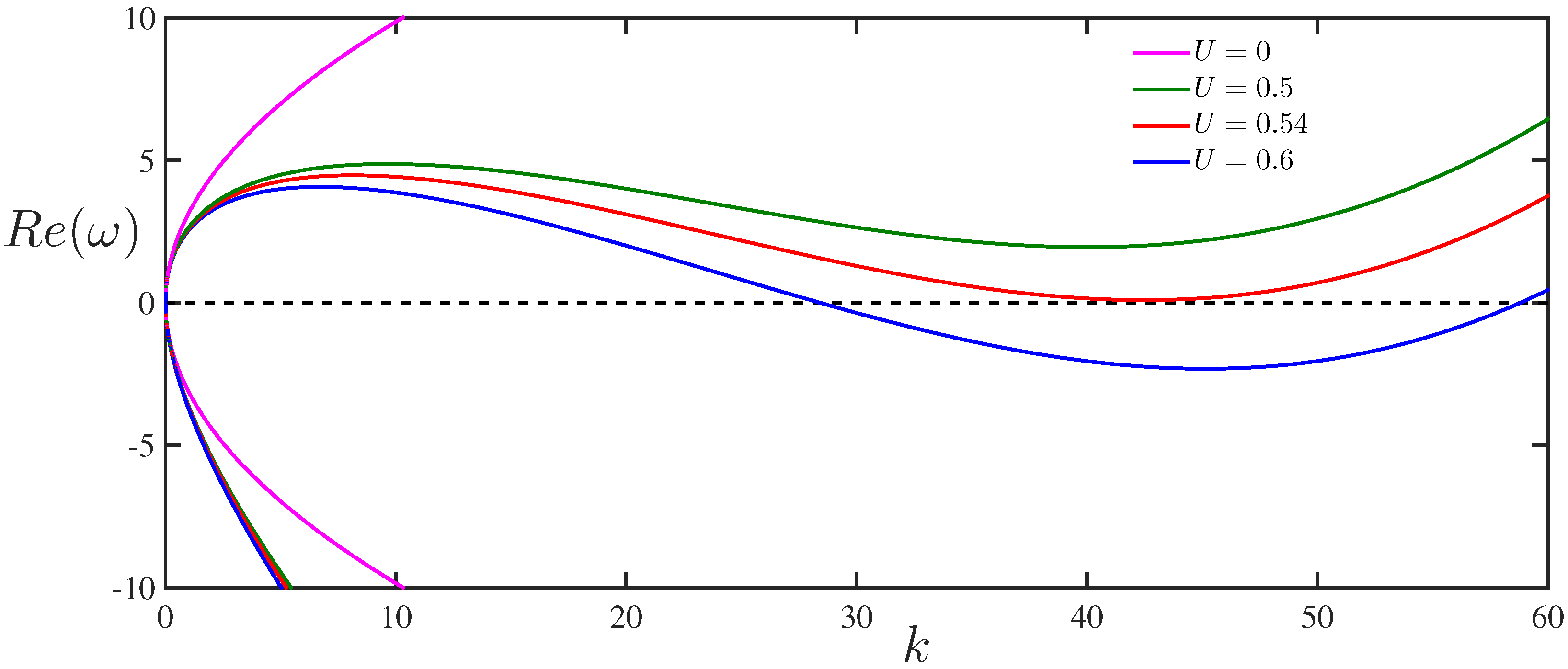
where $a={\rho }_1/{\rho }_2$ is the stratification ratio, $r={\rho }_i/{\rho }_2$ and + and − sign correspond to ${\omega }_1$ and ${\omega }_2$, respectively. The dispersion curves are exhibited in Figure 2 for different values of wind velocity U. For simplicity, the wavenumber k is assumed to be positive, whilst the frequency $\omega$ might be positive or negative. It may be noted that the wave frequency $\omega$ is a positive quantity from a physical standpoint, however, the wavenumber $k\in (-\infty ,\infty )$ might have either sign.

As a special case for $U=0$, Equation (9) describes two symmetric branches of the dispersion curve with respect to the k-axis, which correspond to the flexural-gravity waves propagating in opposite directions with phase speeds of $V_{ph}={\omega }_{1,2}/k$ (see Figure 2).

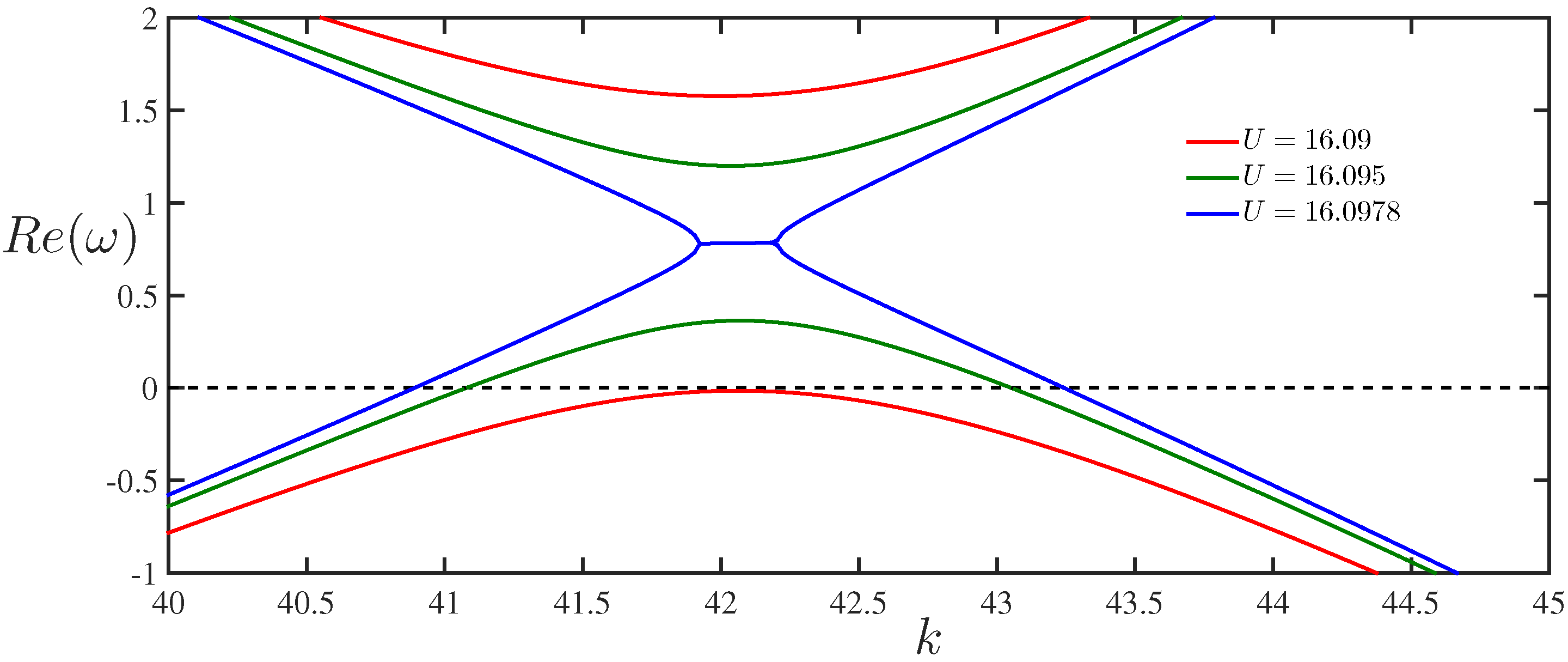
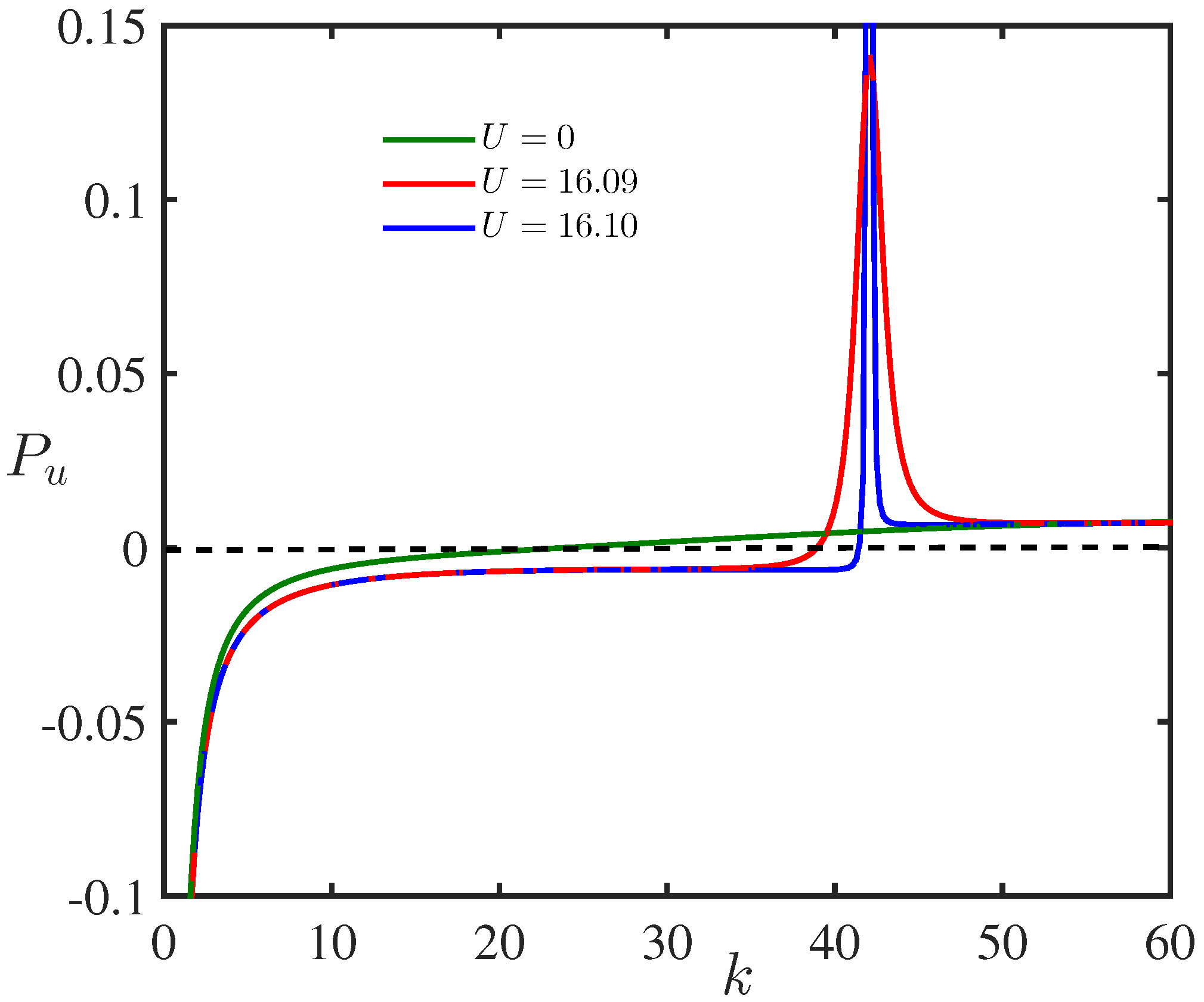
On the other hand, the dispersion curves become non-symmetric for $U\ne 0$ due to the wave drift induced by flow. Further, the lower branch of the dispersion curves changes it sign and become positive in the interval $k_1^{\prime }<k<k_2^{\prime }$ for $U>U_{c1}(=16.09)$ m/s. This is illustrated in Figure 3 for $U=16.095$ m/s, which represents the magnified portion of Figure 2.

Besides, the values of $k_1^{\prime }$ and $k_2^{\prime }$ can be obtained from Equation (9) which are real roots of the fourth-degree polynomial in wavenumber k as given by

$$\begin{array}{c}\hfill {\displaystyle \frac{D}{{\rho }_2}}{k}^4-a{U}^{2}k+(1-a)g=0.\end{array}$$

(10)

Equation (10) can be rewritten in the non-dimensional form as given by

$$\begin{array}{c}\hfill p\left(\kappa \right)\equiv {\kappa }^4-V^2\kappa +1=0,\end{array}$$

(11)

with $\kappa =k{\left\{D/\left[(1-a)g{\rho }_2\right]\right\}}^{1/4}$ and $V^2=(U^{2}a{\rho }_2/D){\left[(1-a)g{\rho }_2/D\right]}^{-3/4}$. Figure 4 reveals that the function $p\left(\kappa \right)$ has no real root for $V<1.7547$, whilst it has two distinct positive real roots for $V>1.7547$.

The critical wind speed $U_{c1}$ is obtained from Equation (9), where both phase and group velocities vanish and are given by

$$\begin{array}{c}\hfill U_{c1}={\left[{\displaystyle \frac{4}{3}}{\displaystyle \frac{1-a}{a}}g{\left({\displaystyle \frac{4D}{a{\rho }_2}}\right)}^{1/3}\right]}^{3/8}.\end{array}$$

(12)

It is pertinent to mention that fragment of the dispersion curves for which the frequency changes its sign corresponds to the negative energy waves (NEWs) [15]. Figure 5 illustrates the same dispersion curves as in Figure 2 for $\omega \ge 0$ with k being of either sign. In this representation, the negative frequency $\omega$ is associated with the negative energy wave. However, the waves with the ’negative frequency’ and negative wavenumber k are qualitatively similar and propagate in the same direction as for waves with positive frequency and positive wavenumber k.

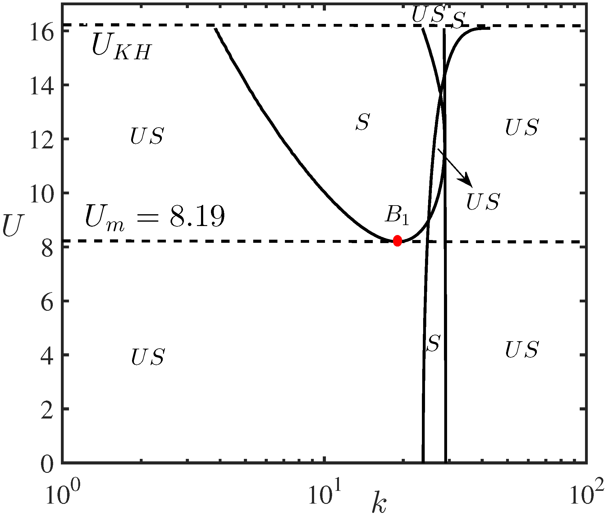
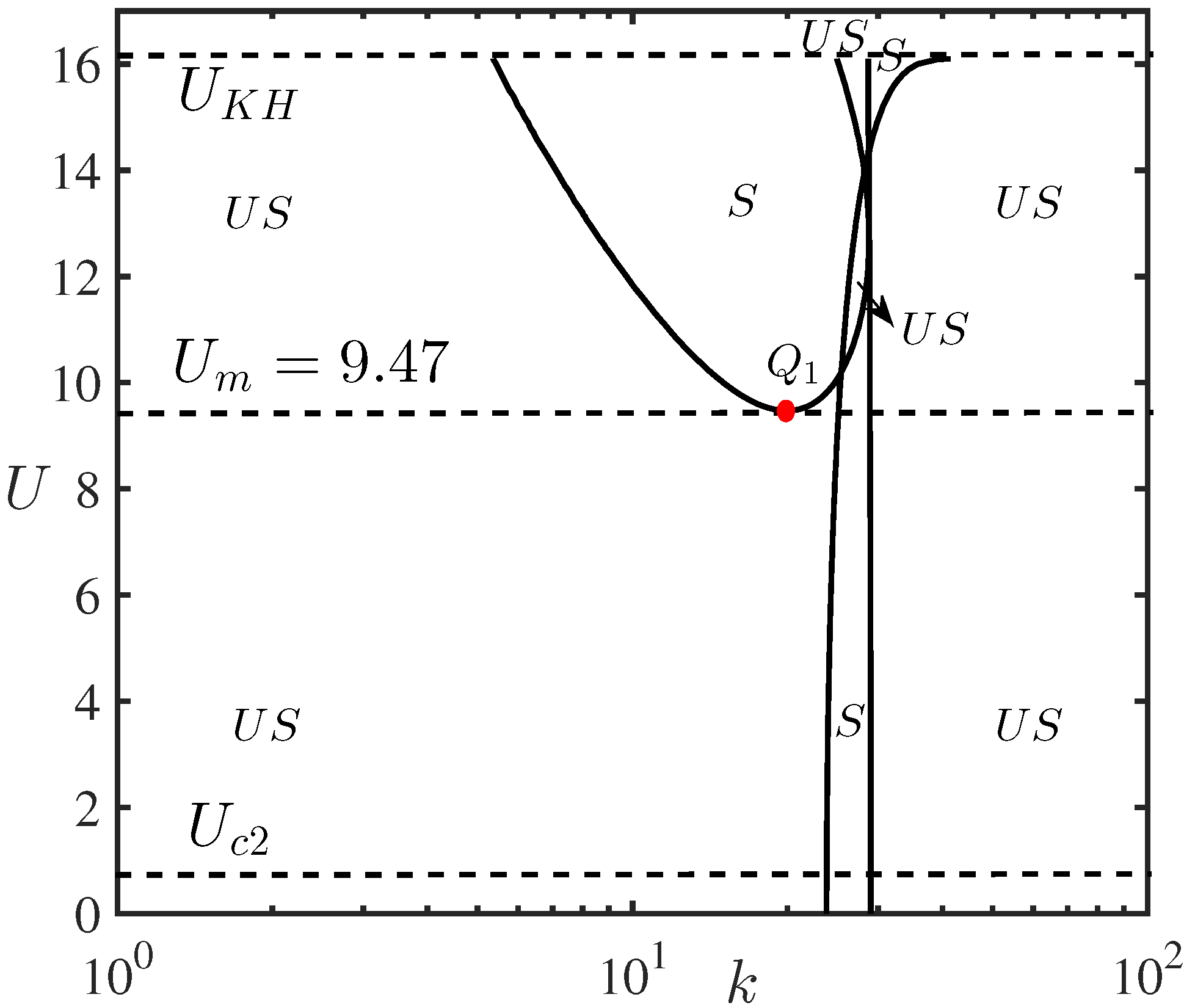
Figure 3 reveals that with an increase in the values of wind speed U beyond $U_{c1}$, the upper and lower branches of the dispersion curves continue to converge to each other and ultimately reconnect at $U=U_{KH}$ where $U_{KH}=U_{c1}\sqrt{1+a}$. It may be noted that the density ratio in the case of air–water interface is chosen as $a=0.0012$ to ensure $U_{KH}\approx 1.0006U_{c1}$. Besides, the Kelvin–Helmholtz-type (K–H) instability occurs when the wind speed U exceeds $U_{KH}$. Moreover, the instability occurs in the interval $k_1\le k\le k_2$, where $k_1$ and $k_2$ can be derived from the following fifth-degree polynomial equation

$$\begin{array}{c}\hfill {\displaystyle \frac{r d D}{{\rho }_2}}{k}^5+(1+a){\displaystyle \frac{D}{{\rho }_2}}{k}^4-a r d U^2{k}^2+\left[(1-a)r d g-a{U}^2\right]k+(1-a^2) g=0.\end{array}$$

(13)

This type of reconnection is significant for the interaction of waves with opposite energy signs which leads to the occurrence of K–H instability [15,16]. This phenomenon is attributed to the exchange of wave energy between the positive and negative energy waves associated with the upper and lower branches of the dispersion relation, respectively. Consequently, the amplitudes of both the waves synchronously grow in time.

Besides, in the interval $U_{c1}<U<U_{KH}$, no K–H instability occurs, whilst there exist non-growing but potentially unstable NEWs (see Figure 3). Further, it may be noted that the wave amplitudes will grow for wavenumber k lying in the range $k_1^{\prime }<k<k_2^{\prime }$ provided their associated energy decreases. Moreover, from Equation (12) it is clear that the velocities $U_{c1}$ and $U_{KH}$ are closed to each other for smaller values of density ratio a, which happens in the case of air–water interface for $a=0.0012$. It is pertinent to mention that Benjamin [22] was the first who discovered that for $a\simeq 1$, $U_{c1}\simeq U_{KH}/\sqrt{2}$, which is typical for internal layers in the oceans or the atmosphere.

Although the parameters for rubber ice are not well defined, it is of interest to demonstrate the influence of these parameters on the dispersion properties of HEWs. In the context of the present study, the value of Young’s modulus is chosen as $E={10}^7$ Pa, which is close to India rubber. Figure 6 illustrates the dispersion curves of HEWs for three different values of Young’s modulus with airflow velocity $U=16.09$ m/s. Figure 6 reveals that the dispersion curve has no optima for $E={10}^6$ Pa, whereas the lower branch of the dispersion curve attains zero minima for $E={10}^7$ Pa and K–H instability occurs for $E={10}^8$ Pa. Thus, it is concluded that the critical wind speed varies with the change in the values of Young’s modulus E which is also clear from Equation (12).

NEWs are neutrally stable in the absence of energy dissipation. However, they can grow in time only if there is a mechanism for taking out their energy. Potentially, there are different mechanisms responsible for the growth of NEWs. In particular, similar to the dissipative instability in plasma [23], viscous dissipation in the immovable lower layer leads to the growth of NEWs [24]. The dissipation of wave energy leading to the growth of NEWs and shear flow instability can be related to the radiation of internal waves from the pycnocline in the density stratified ocean [25]. For amplification of NEWs, viscosity must lead to “positive losses”. For example, the NEWs in the model considered is damped if the upper moving layer is viscous rather than the lower layer. On the other hand, as the viscosity in the moving upper layer leads to “negative damping", the positive energy waves can grow on the upper branch of the dispersion curve. Undoubtedly, when the upper layer is at rest in the reference system, the energy associated with the growth as well as dissipative modes change signs simultaneously [15]. In such a reference system, NEWs exist on the upper branch of the dispersion curve, which can grow under the influence of positive dissipation. Besides, the shear flow instability associated with this mode remains unchanged to the choice of the reference system.

It is interesting to note that by using simple transformation $\omega \to \omega +kU$ in Equation (8), the dispersion relation associated with the stationary upper layer and oppositely moving lower layer can be obtained as

$$G_2(\omega ,k)\equiv {\displaystyle \frac{{\rho }_1}{k}}{\omega }^2+{\displaystyle \frac{{\rho }_2}{k}}\left(1+r d k\right){(\omega +kU)}^2+({\rho }_1-{\rho }_2)g-D{k}^4=0.$$

(14)

Proceeding in a similar manner as in the case of Equation (12), it can be easily concluded that NEWs arise for a very small velocity of the moving lower layer with current speed $U>U_{c2}$ where

$$\begin{array}{c}\hfill U_{c2}={\left[{\displaystyle \frac{4}{3}}{\displaystyle \frac{1-a}{a}}g{\left({\displaystyle \frac{4D}{{\rho }_2}}\right)}^{1/3}\right]}^{3/8}.\end{array}$$

(15)

It is noteworthy to mention that the critical velocities $U_{c1}$ and $U_{c2}$ as in Equations (12) and (15) are very close to each other in the case of $a\simeq 1$ (e.g., for internal waves on the ocean pycnocline). However, it is significant for $a\ll 1$ where $U_{c1}$ is much greater than $U_{c2}$ with $U_{c2}\approx 0.545$ m/s and $U_{c1}\approx 16.09$ m/s as considered in the present study. A fragment of the dispersion curve associated with Equation (14) in the frame co-moving with the upper layer (i.e., static upper layer and moving lower layer) is exhibited in Figure 7 for different values of U including $U_{c2}=0.545$ m/s. In general, Figure 7 reveals that the NEWs can exist on both branches of the dispersion curves for waves that are slowed down relative to the flow with phase velocities being lower than the velocities of the associated fluid layer.

3. The Analysis of Modulation Instability of HEWs

In this section, the expressions for the dispersion coefficient P and nonlinear coefficients Q, as defined in Equation (A20), will be considered in detail for the lower and upper branches of the dispersion curves associated with Equation (9), to determine the criteria of modulation instability.

3.1. The NLS Equation and Modulation Instability in the Lower Branch of the Dispersion Curve

In this subsection, we use the frequency ${\omega }_2$ that corresponds to the lower branch of the dispersion relation (9) to derive the expressions for the dispersion coefficient $P_l$ and the nonlinear coefficient $Q_l$ in the NLS Equation (A20). Then, we obtain:

$$\begin{array}{cc}\hfill P_l& ={\displaystyle \frac{A^2}{8B^{3/2}(1+a+R)}}-{\displaystyle \frac{r^2{d}^2(\sqrt{B}-a k U)}{{(1+a+R)}^3}}-{\displaystyle \frac{r d\left(a U+A/\sqrt{4B}\right)}{{(1+a+R)}^2}}\hfill \\ & +{\displaystyle \frac{2a{U}^2(1+R)+2r d C-20(1+a+R)D{k}^3/{\rho }_2+4a r d k U^2}{4\sqrt{B}(1+a+R)}},\hfill \end{array}$$

(16)

$$\begin{array}{cc}\hfill Q_l& =-{\displaystyle \frac{k^2}{2\sqrt{k(D{k}^4+g{\rho }_2-ag{\rho }_2)B_1-C_1{\rho }_2^2}}}\hfill \\ \hfill \times & \left\{F_{1}k+{\displaystyle \frac{2{\rho }_2{\left[a{\left(kU+{\rho }_2{\displaystyle \frac{A_1}{B_1}}\right)}^2-{\rho }_2{R}_1{\displaystyle \frac{A_1^2}{B_1^2}}\right]}^2}{(1-a)gk+16k^5{\displaystyle \frac{D}{{\rho }_2}}-2a{\left(kU+{\rho }_2{\displaystyle \frac{A_1}{B_1}}\right)}^2-2{\rho }_2^2\left(1+2d k r\right){\displaystyle \frac{A_1^2}{B_1^2}}}}\right\},\hfill \end{array}$$

(17)

where

$$\begin{array}{ccc}\hfill A& =& (1+a+R)C-r d F+2a U^2(1+F)k+a r d k^2{U}^2,\hfill \\ \hfill B& =& (1+a+R)F-a k^2{U}^2(1+R),\hspace{1em}C=g(a-1)-5D{k}^4/{\rho }_2,\hfill \\ \hfill F& =& D{k}^5/{\rho }_2+(1-a)gk,\hspace{1em}R=r d k,\hfill \\ \hfill A_1& =& \sqrt{k{B}_1{F}_1/{\rho }_2^2-C_1}-akU,\hspace{1em}{B}_1=(1+a){\rho }_2+\rho d k,\hfill \\ \hfill C_1& =& a k^2{U}^2{R}_1/{\rho }_2,\hspace{1em}{F}_1=D{k}^4+(1-a){\rho }_{2}g,\hspace{1em}{R}_1={\rho }_2+\rho d k.\hfill \end{array}$$

In particular, for $a=U=D={\rho }_i=0$, the dispersion relation (9), corresponding group velocity, dispersion and nonlinear coefficients $P_l$ and $Q_l$ reduce to:

$${\omega }_2=-\sqrt{gk},\hspace{1em}{c}_g=-\frac{1}{2}\sqrt{{\displaystyle \frac{g}{k}}},\hspace{1em}{P}_l={\displaystyle \frac{1}{8}}\sqrt{{\displaystyle \frac{g}{k^3}}},\hspace{1em}{Q}_l={\displaystyle \frac{1}{2}}\sqrt{g{k}^5},$$

(18)

where the coefficients $P_l$ and $Q_l$ are analogous to the coefficients of the NLS equation for surface gravity waves in deep water [26,27,28]. Note also that the dispersion and nonlinear coefficients of the NLS equation for flexural-gravity waves in deep water [13] follow from Equations (16) and (17) by setting $a=0$ and $U=0$.

In Figure 8 and Figure 9, the dependencies of $P_l\left(k\right)$ and $Q_l\left(k\right)$ are shown for the lower branch of the dispersion curve for three different values of wind speed, $U=0$ m/s, $U=U_{c1}=16.09$ m/s and $U=U_{KH}\approx 16.10$ m/s. Figure 8 reveals that for all values of U the dispersion coefficient $P_l\left(k\right)$ has only one root where its sign changes from positive to negative. On the other hand, Figure 9 reveals that the nonlinear coefficient $Q_l\left(k\right)$ for all values of U has a singularity at $k=k_s\approx 29.1$1/m where $Q_l\left(k\right)$ changes its sign from positive to negative. It is worth mentioning that both the functions $P_l\left(k\right)$ and $Q_l\left(k\right)$ attain their minima around the point $k\approx 42$.1/m where K–H instability occurs for $U=U_{KH}$. The minima become deeper and deeper when U approaches $U_{KH}$, and in the limit, $U\to U_{KH}$, the singularities appear in both the functions $P_l\left(k\right)$ and $Q_l\left(k\right)$.

As per the Lighthill criterion, a uniform wavetrain becomes unstable with respect to self-modulation in the case of the function $W_l\left(k\right)\equiv P_l\left(k\right)Q_l\left(k\right)$ is positive [29,30]. Figure 10 demonstrates the zones of modulation stability (S) and instability ($US$) in the $(k,U)$ plane. Furthermore, a dramatic change in the stability diagram is observed for the wind speed U higher than the critical value $U_m=8.19$ m/s, which is caused by several sign changes of the nonlinear coefficient $Q_l\left(k\right)$ when $U>U_m$. Figure 10 shows, in particular, zones of the modulation instability for flexural-gravity waves in deep-water when $U=0$ and $a=0$ [13].

It is worth mentioning that the maximum growth rate of modulation instability occurs for the wavenumber of modulation $K_{max}=b_0\sqrt{Q_l/P_l}$ in the NLS Equation (A20), where $b_0$ is referred as the sinusoidal wave amplitude (see, e.g., [31]). Further, it is important to note that $I_{max}=\left|Q_l\left(k\right)\right|b_0^2$ is the maximal value of the growth rate. For a given value of U, this expression can be further optimized with respect to the carrier wavenumber k [32].

In the course of the development of modulation instability, envelope solitary waves (solitons), breathers, freak waves can emerge from certain initial perturbations; the detailed description of fascinating phenomena related to the interactions of such formations can be found in Refs. [8,26,33]. In the case of modulational stability, dark solitons can be developed on the background of a quasi-sinusoidal wave [8]. Figure 11 demonstrates the examples of (a) bright and (b) dark solitary envelope waves.

The NLS Equation (A20) becomes inapplicable when its coefficients $P\left(k\right)$ or $Q\left(k\right)$ vanish. This occurs at the boundaries between the domains of stability and instability shown in Figure 10. In such a case, the generalised NLS equation should be derived by taking into account the higher-order terms as in Refs. [34,35]. However, this is not considered in the present study and will be studied separately.

3.2. The NLS Equation and Modulation Instability in the Upper Branch of the Dispersion Curve

Now let us use the frequency ${\omega }_1$ that corresponds to the upper branch of the dispersion relation (9) for the derivation of the dispersion and nonlinear coefficients $P_u$ and $Q_u$ and to determine the condition of modulation instability. As in the case of the lower branch of the dispersion relation, the dispersive coefficient $P_u$ and the nonlinear coefficient $Q_u$ in the NLS Equation (A20) are obtained as:

$$\begin{array}{cc}\hfill P_u& ={\displaystyle \frac{-1}{(1+a+R)}}\left[{\displaystyle \frac{A^2}{4B^{3/2}}}-{\displaystyle \frac{r^2{d}^2(\sqrt{B}+a k U)}{{(1+a+R)}^2}}+{\displaystyle \frac{r d}{1+a+R}}\left(a U-{\displaystyle \frac{A}{2\sqrt{B}}}\right)\right.\hfill \\ & \left.+{\displaystyle \frac{2a U^2(1+R)+2r d C-20(1+a+R)D{k}^3/{\rho }_2+4a r d k U^2}{2\sqrt{B}}}\right],\hfill \end{array}$$

(19)

$$\begin{array}{cc}\hfill Q_u& ={\displaystyle \frac{k^2}{2\sqrt{k(D{k}^4+g {\rho }_2-a g {\rho }_2)B_1-C_1{\rho }_2^2}}}\hfill \\ & \times \left\{F_{1}k+{\displaystyle \frac{2{\rho }_2{\left[a{\left(Uk-{\rho }_2{\displaystyle \frac{P_1}{B_1}}\right)}^2-{\rho }_2{R}_1{\displaystyle \frac{P_1^2}{B_1^2}}\right]}^2}{(1-a)g k+16k^5{\displaystyle \frac{D}{{\rho }_2}}-2a{\left(k U-{\rho }_2{\displaystyle \frac{P_1}{B_1}}\right)}^2-2{\rho }_2^2\left(1+2d k r\right){\displaystyle \frac{P_1^2}{B_1^2}}}}\right\},\hfill \end{array}$$

(20)

where $A,B,C,R,B_1,C_1,F_1$ and $R_1$ are the same as in Equations (16) and (17) with $P_1=\sqrt{k{B}_1{F}_1/{\rho }_2^2-C_1}+a k U$. The coefficients $P_u$ and $Q_u$ are exhibited in Figure 12 and Figure 13. A comparison of Figure 8 and Figure 9 with that of Figure 12 and Figure 13 reveals that the trend of the dispersion and nonlinear coefficients for the upper branch of the dispersion curves are opposite to that of $P_l$ and $Q_l$.

Equations (19) and (20) attribute that the modulational instability occurs for positive values of the function $W_u\left(k\right)\equiv P_u\left(k\right)Q_u\left(k\right)$ associated with the upper branch of the dispersion curve. Figure 14 demonstrates the zones in $(k,U)$-plane where the function $W_u\left(k\right)$ is positive, and that leads to the occurrence of modulation instability. Further, the graphic begins to alter dramatically when U exceeds a critical limit $U_m=9.4719$ m/s, which is caused again by multiple changes of sign of the nonlinear coefficient $Q_u$ when $U>U_m$. It is evident from Figure 10 and Figure 14 that the domains of modulation stability and instability are bizarrely interspersed on the diagram when U exceeds the critical value $U_m$ in each branch of the dispersion curve. The importance of highlighting such domains is in the understanding of the existence of bright and dark solitary envelope waves. The former can arise in the process of the development of modulation instability, whereas the latter can appear in the modulationally stable regions on the parameter plane. Moreover, in the case of modulation instability, rogue waves with extremely high amplitudes can emerge from rather regular initial perturbations [33]. The most important conclusion which can be derived from this study is the existence of modulationally unstable waves of negative energy for wind speed in the range $U_{c2}<U<U_m$. Such waves can grow in time if a dissipative mechanism extracting energy from such waves is taken into account. This can be, for example, a turbulent viscosity of air which can be very high in comparison with the molecular viscosity even at the relatively weak wind. However, this issue is beyond the scope of the present study.

4. Conclusions

In the present paper, the criteria for modulation instability of hydro-elastic waves on the air–water interface have been investigated under the influence of wind. The consideration was carried out within the framework of the simplest model of wind with the uniform profile and tangential velocity discontinuity. However, this is a widely used canonical model of the flow in hydrodynamics, physical oceanography, geophysical fluid dynamics, plasma physics, and other fields. Despite the simplicity, the model provides an insight into the complicated range of phenomena occurring in the wave-current interactions. To the best of the authors’ knowledge, the modulation instability of hydro-elastic waves under the influence of wind was not studied thus far. Thus, the present study has filled the said gap on modulation instability in the literature. The study exhibits the wavenumber range based on the current speed in which the stability and instability can occur in the lower and upper branches of the dispersion relation. From the general model investigated here, the limiting cases of pure gravity waves or flexural-gravity waves without airflow are reproduced. It is important to note that within the model with the uniform velocity profile, the boundary layer effects at the air–water interface are neglected. This is acceptable for long perturbations with wavelengths much greater than the typical thickness of the boundary layer. Therefore, our analysis is not applicable to waves with large wavenumbers.

As a summary, an estimate of parameters of a modulated wave are presented with wavenumber $k=10$.1/m ($\lambda =2\pi /k\approx 0.63$ m), amplitude ${\eta }_0=0.01$ m and $U=1$ m/s. Subsequently, the most rapidly increasing modulation wavenumber $K_{max}={\eta }_0\sqrt{Q_u/P_u}\approx 2.01$1/m and wavelength $\Lambda =2\pi /K_{max}\approx 3.12$ m are obtained. The maximal value of the growth rate is found to be $I_{max}=\left|Q\left(k\right)\right|{\eta }_0^2\approx 0.05$1/s along with the characteristic time of wave growth $\tau =1/I_{max}\approx 20.4$ s. These parameters look reasonable for the rubber ice and, they are practically insensible to the variation of the wind speed in the interval $U_{c2}<U<U_m$. The study can be generalized to deal with complex flow patterns including turbulent viscosity of air as well as the role of lateral compressive force on the floating ice sheet.

References

1. Available online: https://news.mail.ru/society/40290629/ (accessed on 10 December 2021).
2. Kheisin, D.Y. Dynamics of Floating Ice Cover (in Russian. Technical English Translation in: FSTC-HT-23-485-69, U.S. Army Foreign Science and Technology Center); Gidrometeoizdat: Leningrad, Russia, 1967. [Google Scholar]
3. Squire, V.A.; Hosking, R.J.; Kerr, A.D.; Langhorne, P.J. Moving Loads on Ice Plates; Kluwer Academic Publishers: Dordrecht, The Netherlands, 1996. [Google Scholar]
4. Sahoo, T. Mathematical Techniques for Wave Interaction with Flexible Structures; CRC Press: Boca Raton, FL, USA, 2012. [Google Scholar]
5. Bukatov, A.E. Waves in a Sea with a Floating Ice Cover; FGBUN MHI: Sebastopol, CA, USA, 2017. (In Russian) [Google Scholar]
6. Djordjevic, V.D.; Redekopp, L.G. On two-dimensional packets of capillary-gravity waves. J. Fluid Mech. 1977, 79, 703–714. [Google Scholar] [CrossRef]
7. Ablowitz, M.J.; Segur, H. On the evolution of packets of water waves. J. Fluid Mech. 1979, 92, 691–715. [Google Scholar] [CrossRef]
8. Ablowitz, M.J.; Segur, H. Solitons and the Inverse Scattering Transform; SIAM: Philadelphia, PA, USA, 1981. [Google Scholar]
9. Boral, S.; Sahoo, T.; Stepanyants, Y. Modulation instability of surface waves in the model with the uniform wind profile. Symmetry 2021, 13, 651. [Google Scholar] [CrossRef]
10. Guyenne, P.; Părău, E.I. Finite-depth effects on solitary waves in a floating ice-sheet. J. Fluids Struct. 2014, 49, 242–262. [Google Scholar] [CrossRef] [Green Version]
11. Il’ichev, A.T. Solitary wave packets beneath a compressed ice cover. Fluid Dyn. 2016, 51, 327–337. [Google Scholar] [CrossRef]
12. Il’ichev, A.T. Effective wavelength of envelope waves on the water surface beneath an ice sheet: Small amplitudes and moderate depths. Theor. Math. Phys. 2021, 208, 1182–1200. [Google Scholar] [CrossRef]
13. Slunyaev, A.; Stepanyants, Y. Modulation property of flexural-gravity waves on a water surface covered by a compressed ice sheet. arXiv 2021, arXiv:2112.07906. [Google Scholar]
14. Landau, L.D.; Lifshits, E.M. Fluid Mechanics; Butterworth-Heinemann: Burlington, MA, USA, 1987. [Google Scholar]
15. Fabrikant, A.L.; Stepanyants, Y.A. Propagation of Waves in Shear Flows; World Scientific Publishing Company: Singapore, 1998. [Google Scholar]
16. Ostrovski, L.A.; Rybak, S.A.; Tsimring, L.S. Negative energy waves in hydrodynamics. Sov. Phys. Uspekhi 1986, 29, 1040. [Google Scholar] [CrossRef]
17. Ezersky, A.B.; Ostrovsky, L.A.; Stepanyants, Y.A. Wave-induced flows and their contribution to the energy of wave motions in a fluid. Izv. Acad. Sci. USSR Atmos. Ocean. Phys. 1981, 17, 890–895. [Google Scholar]
18. Miles, J.W. On the reflection of sound at an interface of relative motion. J. Acoust. Soc. Am. 1957, 29, 226–228. [Google Scholar] [CrossRef]
19. Ribner, H.S. Reflection, transmission and amplification of sound by a moving medium. J. Acoust. Soc. Am. 1957, 29, 435–441. [Google Scholar] [CrossRef]
20. Gelash, A.; Agafontsev, D.; Zakharov, V.; El, G.; Randoux, S.; Suret, P. Bound state soliton gas dynamics underlying the noise-induced modulational instability. Phys. Rev. Lett. 2019, 123, 234102. [Google Scholar] [CrossRef] [Green Version]
21. Ducrozet, G.; Slunyaev, A.; Stepanyants, Y. Transformation of envelope solitons on a bottom step. Phys. Fluids 2021, 33, 066606. [Google Scholar] [CrossRef]
22. Benjamin, T.B. The threefold classification of unstable disturbances in flexible surfaces bounding inviscid flows. J. Fluid Mech. 1963, 16, 436–450. [Google Scholar] [CrossRef]
23. Nezlin, M.V. Negative-energy waves and the anomalous Doppler effect. Sov. Phys. Uspekhi 1976, 19, 946. [Google Scholar] [CrossRef]
24. Cairns, R.A. The role of negative energy waves in some instabilities of parallel flows. J. Fluid Mech. 1979, 92, 1–14. [Google Scholar] [CrossRef]
25. Ostrovsky, L.A.; Stepanyants, Y.A.; Tsimring, L.S. Radiation instability in a stratified shear flow. Int. J. Non-Lin. Mech. 1983, 19, 151–161. [Google Scholar] [CrossRef]
26. Yuen, H.C.; Lake, B.M. Nonlinear dynamics of deep-water gravity waves. In Advances in Applied Mechanics; Elsevier: Amsterdam, The Netherlands, 1982; Volume 22, pp. 67–229. [Google Scholar]
27. Peregrine, D.H. Water waves, nonlinear Schrödinger equations and their solutions. ANZIAM J. 1983, 25, 16–43. [Google Scholar] [CrossRef] [Green Version]
28. Stiassnie, M. Note on the modified nonlinear Schrödinger equation for deep water waves. Wave Motion 1984, 6, 431–433. [Google Scholar] [CrossRef]
29. Lighthill, M.J. Contributions to the theory of waves in nonlinear dispersive systems. IMA J. Appl. Math. 1965, 1, 269–306. [Google Scholar] [CrossRef]
30. Lighthill, M.J. Waves in Fluids; Cambridge University Press: Cambridge, UK, 1978. [Google Scholar]
31. Ostrovsky, L.A.; Potapov, A.I. Modulated Waves: Theory and Applications; The Johns Hopkins University Press: Baltimore, MD, USA, 2002. [Google Scholar]
32. Grimshaw, R.; Stepanyants, Y. Emergence of envelope solitary waves from the initial lo-calised pulses within the Ostrovsky equation. Radiophys. Quantum Elect. 2020, 63, 21–28. [Google Scholar] [CrossRef]
33. Kharif, C.; Pelinovsky, E.; Slunyaev, A. Rogue Waves in the Ocean; Springer: Berlin/Heidelberg, Germany, 2009. [Google Scholar]
34. Dysthe, K.B. Note on a modification to the nonlinear Schrödinger equation for application to deep water waves. Proc. R. Soc. Lond. A 1979, 369, 105–114. [Google Scholar]
35. Trulsen, K.; Dysthe, K.B. A modified nonlinear Schrödinger equation for broader bandwidth gravity waves on deep water. Wave Motion 1996, 24, 281–289. [Google Scholar] [CrossRef]
36. Abourabia, A.M.; Mahmoud, M.A.; Khedr, G.M. Solutions of nonlinear Schrödinger equation for interfacial waves propagating between two ideal fluids. Can. J. Phys. 2009, 87, 675–684. [Google Scholar] [CrossRef]
Figure 1. Schematic sketch of the airflow model with the tangential discontinuity above the ice covered deep water.
Fluids 06 00458 g001
Figure 2. Graphics of the dispersion relations ω 1 ( k ) (upper branches) and ω 2 ( k ) (lower branches) for the ice parameters presented above – see after Equation (5); the values of U are shown in m/s.
Fluids 06 00458 g002
Figure 3. The magnified fragment of Figure 2 for the same set of parameters.
Fluids 06 00458 g003
Figure 4. (Color online) The shape of the polynomial p ( κ ) for three different values of V. Line 1, V = 0.7 ,—no real roots; line 2, V = 1.7547 ,—there is one double root (designated by red dot); line 3, V = 2.0 ,—there are two real roots (designated by blue dots).
Fluids 06 00458 g004
Figure 5. Non-symmetric branches of dispersion curves corresponding to waves propagating in the opposite direction. Note that the pink and blue lines have negative portions, which correspond to NEWs.
Fluids 06 00458 g005
Figure 6. Influence of ice elasticity on the dispersion curves for the particular airflow velocity U = 16.09 m/s.
Fluids 06 00458 g006
Figure 7. Dispersion relation (14) in the frame co-moving with the upper layer (air) for a few values of U.
Fluids 06 00458 g007
Figure 8. (Color online) Variation of dispersion coefficient P l ( k ) versus wavenumber k for different values of wind speed in the case of the lower branch of the dispersion curve.
Fluids 06 00458 g008
Figure 9. (Color online) Variation of the nonlinear coefficient Q l versus wavenumber k for different values of wind speed U in the case of lower branch of dispersion curve.
Fluids 06 00458 g009
Figure 10. Zones of modulation stability (S) and instability ( U S ) in the ( k , U ) plane. The dashed line on the top depicts the critical velocity U K H = 16.10 1/m at which the Kelvin–Helmholtz instability arises. The bifurcation point in the diagram is denoted by B 1 for U = U m .
Fluids 06 00458 g010
Figure 11. (Color online) Examples of (a) bright and (b) dark envelope solitons.
Fluids 06 00458 g011
Figure 12. (Color online) Variation of the dispersion coefficient P u versus wavenumber k for different values of wind speed in the case of upper branch of dispersion curve.
Fluids 06 00458 g012
Figure 13. (Color online) Variation of the nonlinear coefficient Q u versus wavenumber k for different values of wind speed in the case of upper branch of dispersion curve.
Fluids 06 00458 g013
Figure 14. Modulation stability (S) and instability ( U S ) zones in the ( k , U ) plane. The dashed line on the top depicts that the velocity corresponds to the K–H instability U K H = 16.0978 m/s. The bifurcation point in the diagram is denoted by Q 1 for U = U m .
Fluids 06 00458 g014
Publisher’s Note: MDPI stays neutral with regard to jurisdictional claims in published maps and institutional affiliations.